A history of TOPMODEL - HESS
←
→
Page content transcription
If your browser does not render page correctly, please read the page content below
Hydrol. Earth Syst. Sci., 25, 527–549, 2021
https://doi.org/10.5194/hess-25-527-2021
© Author(s) 2021. This work is distributed under
the Creative Commons Attribution 4.0 License.

A history of TOPMODEL
Keith J. Beven1 , Mike J. Kirkby2 , Jim E. Freer3,4 , and Rob Lamb5,1
1 Lancaster Environment Centre, Lancaster University, Lancaster, UK
2 School of Geography, University of Leeds, Leeds, UK
3 University of Saskatchewan, Centre for Hydrology, Canmore, Canada
4 School of Geographical Sciences, University of Bristol, Bristol, UK
5 JBA Trust, Broughton, UK

Correspondence: Keith Beven (k.beven@lancaster.ac.uk)

Received: 6 August 2020 – Discussion started: 25 August 2020
Revised: 17 November 2020 – Accepted: 18 November 2020 – Published: 2 February 2021

Abstract. The theory that forms the basis of TOPMODEL                    ticularly runoff generation on a variable contributing area. It
(a topography-based hydrological model) was first outlined               did so in a structurally, parametrically, and computationally
by Mike Kirkby some 45 years ago. This paper recalls some                parsimonious model which gave it advantages over the full
of the early developments, the rejection of the first journal            implementation of the physically based model blueprint set
paper, the early days of digital terrain analysis, model cali-           out by Freeze and Harlan (1969).
bration and validation, the various criticisms of the simpli-               The story of TOPMODEL starts when Mike Kirkby (MK)
fying assumptions, and the relaxation of those assumptions               was at the University of Bristol, where he worked with his
in the dynamic forms of TOPMODEL. A final section ad-                    PhD student Darrel Weyman in the East Twin catchment
dresses the question of what might be done now in seeking a              in the Mendips. One critical observation from Darrel Wey-
simple, parametrically parsimonious model of hillslope and               man’s work was the synchronicity of flows in a throughflow
small catchment processes if we were starting again.                     trough and in the main channel, suggesting the possibility
                                                                         that subsurface runoff per unit area might be approximately
                                                                         spatially constant, which is a key underlying assumption of
1   TOPMODEL: the background                                             TOPMODEL. While this may not be a general expectation,
                                                                         the consequent analysis of the response of the upper East
TOPMODEL (a topography-based hydrological model) is a                    Twin led to the concept of a topographic index (as a/tanβ,
rainfall-runoff model that has its origins in the recognition of         with a as upslope contributing area per unit contour length
the dynamic nature of runoff contributing areas in the 1960s             and tanβ as local slope).
and 1970s that had been revealed in the data analysis of par-               The first theoretical statement of TOPMODEL was pre-
tial area contributions of Betson (1964) in Tennessee, USA;              sented in Kirkby (1975). He wrote the following there:
the field experience of Dunne and Black (1970) in Vermont,
USA; and Weyman (1970, 1973) in the Mendips, UK. It was                       Any model with only a few parameters must nec-
one of the very first models to make explicit use of topo-                    essarily simplify the spatial variation of moisture
graphic data in the model formulation and hence the name of                   content over a drainage basin. For a given average
the model (Beven and Kirkby, 1979, hereafter BK79). This                      moisture content, there is a wide range of possi-
was, however, well before digital terrain or elevation maps                   ble spatial distributions, even if rainfall is always
started to be made available.1 The theory of TOPMODEL                         spatially uniform, as is assumed here. To predict
aimed to reflect the way in which the topography of a catch-                  the spatial consequences of an average moisture
ment would shape the dynamic process responses and par-                       level, some assumptions must be made about the
   1 It was also before the term “top model” started to be used in the   with the name at EGU when the first Italian issue of TOPMODEL
fashion industry, though Ezio Todini was quick to have some fun          magazine was published.

Published by Copernicus Publications on behalf of the European Geosciences Union.
528 K. J. Beven et al.: A history of TOPMODEL
duration of the rainfall inputs. The simplest, which
is adopted here, is to assume a time-independent
steady state of net rainfall input, ı (p. 81).
Then, using the original nomenclature of Kirkby (1975),
at any point, downslope flow per unit contour length, q, will
be given by a (ı − qo ), where a is the upslope contributing
area to that point, and qo is a constant rate of leakage to the
subsoil. When making the further assumptions that the local
hydraulic gradient can be approximated by the slope angle,
tan β, and the local transmissivity can be represented as KS,
where K is a permeability per unit of storage and S is the
local saturated zone storage in rainfall equivalent depth units,
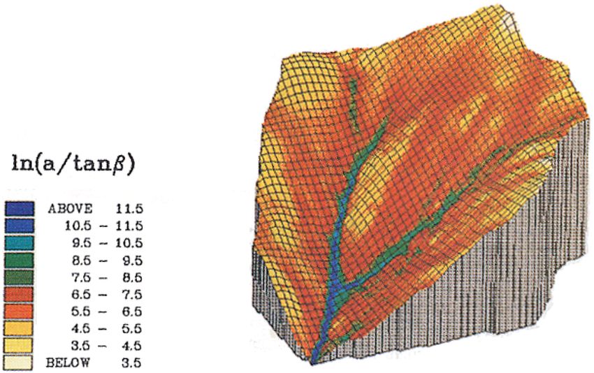
Figure 1. Distribution of the topographic index (a/ tan β) for the
then upper East Twin catchment, Mendips, UK (from Kirkby, 1975, with
permission from Pearson Publishers).
q = a (ı − qo ) = KS tan β (1)
or catchment area A. Combining Eqs. (3) and (4) gives a con-
dition for soil saturation in terms of the topographic index
S = a (ı − qo ) /K tan β. (2)
a/ tan β at all points where
KS is then an effective transmissivity of the soil at a stor- a λKSo
age of S. Note that this assumes that the hydraulic gradi- > . (5)
tan β K̄ S̄
ent tan β is defined with respect to the plan distance, while
infiltration and drainage rates are defined with respect to The topographic index can be mapped in a catchment area as
plan unit area. Others have suggested that the use of sin β a function of the topography; it then gives an indication of
is more correct, i.e. relative to distance along the hillslope, where a saturated contributing area might occur and how it
so that transmissivity is defined by the plane orthogonal to might spread as a function of storage (e.g. Fig. 1 for the upper
the slope rather than horizontally (e.g. Montgomery and Di- East Twin). The expression is simplified further if the perme-
etrich, 1994, 2002; Borga et al., 2002; Chirico et al., 2003). ability can be considered spatially constant and λ simplifies
Clearly this makes little difference for low to moderate slope to the mean value of the topographic index in the catchment.
angles, while for high slope angles it is unlikely that a water The topographic index was also used later to compare with
table would be parallel to the surface so that this assump- the saturated areas at Tom Dunne’s Sleepers River field site
tion would break down. In addition, any difference in the in Vermont in Kirkby (1978) (Fig. 2). Kirkby (1975) also
definition of transmissivity is likely to be smaller than the provides relationships for the leakage term qo and routing
uncertainty with which transmissivities can be estimated or through a channel network based on the network width func-
calibrated. tion.
Equation (2) allows the condition for the soil to be just In this form, TOPMODEL does not require a steady rain-
saturated to the surface at a storage of So to be defined as fall duration long enough to reach steady state but only that
the storage for any given value of S takes up a form as if it
a So was at a steady state with a steady homogeneous recharge
S = So or = . (3)
K tan β (ı − qo ) rate over the upslope contributing area to any point in the
catchment. This implies that as storage changes, the celeri-
In terms of water balance accounting for the catchment as a ties in the saturated zone are fast enough that the transition
whole, it is useful to integrate the expression for S to provide between configurations with changes in storage are relatively
a catchment average value S. rapid. This will be more likely in wet, relatively shallow soils
λ (ı − qo ) on moderate slopes and where soil permeabilities increase
S= , with depth of saturation. There will be no expectation of a
K water table being parallel to the surface on deeper subsurface
where systems on low slope or on very high slopes where more lo-
K
Z
a calised saturation will occur at the base of the slope. How-
λ= dA. (4) ever, where the soil profile is much shallower than the length
A K tan β
of the slope then any build-up of saturation at the base of
Expressing the relationship for S in this way allows for the profile under wet conditions must be fairly parallel to the sur-
potential for local permeability to vary while the effective face. This might break down under drier conditions or where
recharge rate is in ratio to the mean permeability K over the there is a loss to deeper layers.
Hydrol. Earth Syst. Sci., 25, 527–549, 2021 https://doi.org/10.5194/hess-25-527-2021K. J. Beven et al.: A history of TOPMODEL 529
where D is the mean storage deficit and λ is now the areal
integral of ln (a/ tan β) with To and m assumed spatially con-
stant. This is the expression used to determine the dynamics
of the saturated contributing area in what might be called the
classical version of TOPMODEL (Fig. 3). Equation (7) im-
plies that when D is zero, all the points with a topographic
index greater than the mean value λ are predicted as satu-
rated. Negative values of D mean that more of the catchment
is predicted as saturated. Redistribution at each model time
step will produce negative local D values on the saturated
area. In the model, accounting for this is treated as return
flow from the saturated zone and is routed to the channel to
properly maintain mass balance. Saulnier and Datin (2004)
suggested that this creates a bias in the prediction of the sat-
urated areas and suggested a formulation that calculates a
deficit only over the unsaturated area of the catchment.
Equation (6) can be integrated along the length of all
reaches in the channel network to provide the integral dis-
charge from the hillslopes in terms of the mean storage deficit
D as
Qb = Qo exp −D/m , (8)
where Qb is the integrated output along all the reaches in
the channel network, Qo = Ae−λ (for the case of a homo-
geneous downslope transmissivity), and A is the catchment
area (see Beven, 2012, p. 214, for a full derivation). To ini-
Figure 2. Comparison of the topographic index tialise the model, this relationship (8) can then be inverted,
(a/ tan β) >160 m2 /m with observed saturated areas after spring given a value of catchment discharge to give the initial mean
snowmelt in the Sleepers River WC-4 catchment, Vermont, USA storage deficit. Note that (8) implies a first-order hyperbolic
(from Kirkby, 1978, with permission from Wiley). shape for the recession limb of the hydrograph. This can be
checked for a particular application by plotting the inverse
of observed discharges against time. This should plot as a
Kirkby (1975) introduced an additional assumption that straight line if (8), and consequently Eq. (6), is valid (Am-
downslope flow could be represented as an exponential func- broise et al., 1996a; Beven, 2012).
tion of storage deficit below saturation, with D in units of It is worth noting here that the deficit D represents a stor-
depth. This is consistent with an assumption of spatially ho- age deficit due to gravity drainage. Any additional deficits
mogeneous subsurface runoff increments at all times up to resulting from evapotranspiration losses are calculated sep-
steady state (Kirkby, 1997). It was also realised that by ex- arately from the various model stores. By the addition of an
pressing the saturated storage in the profile in terms of stor- additional parameter of available storage for gravity drainage
age deficit rather than water table depth, one parameter could per unit depth of soil (which can be related to the concept of
be eliminated. At that time, the issue of designing models to “field capacity”), the deficit D can be converted to a depth
facilitate the calibration problem and reduce the potential for to the saturated zone. Thus the model can be equally formu-
overfitting was already the subject of discussion in the litera- lated in terms of water table depths, and there are a variety of
ture (Ibbitt and O’Donnell, 1971, 1974; Kirkby 1975; John- applications that have used the model in this way to compare
ston and Pilgrim, 1976). Thus against observed depths of saturation (e.g. Sivapalan et al.,
1987; Lamb et al., 1997, 1998; Seibert et al., 1997; Blazkova
q = To tan β exp (−D/m) , (6) et al., 2002; Freer et al., 2004).
The topographic index acts as an index of hydrological
where To is the downslope transmissivity when the soil is just similarity (Beven et al., 1995; Beven, 2012) resulting from
saturated to the surface, and m is a parameter also with units the assumption of homogeneous recharge to the saturated
of depth. Following the same derivation as above gives the zone at any point in time. The elegance of the similarity ap-
condition for saturation as proach means that it is not necessary to make calculations
for every point in the catchment buy only for representative
a D values of the index, which can then be weighted by the distri-
ln > − λ, (7) bution function. This was particularly important when com-
tan β m
https://doi.org/10.5194/hess-25-527-2021 Hydrol. Earth Syst. Sci., 25, 527–549, 2021530 K. J. Beven et al.: A history of TOPMODEL Figure 3. Schematic of the classical version of TOPMODEL (see Table 1 for the definition of the parameters). puter power was limited in the 70s and 80s but remains use- 1995). This was controlled by a time delay per unit of deficit ful in applications to large catchments and when ensembles parameter, td . of runs are required for uncertainty estimation. Good reso- In respect of routing the surface and channel flows, there lution is required at the higher end of the distribution where was one thing that KB got wrong in the original BK79 model the contributing area first starts to spread, but experience with formulation. It used a form of explicit non-linear time delay the model suggested that about 30 representative values was routing for the overland flow and channel network that will generally sufficient for convergence of the calculated outputs produce kinematic shocks at times when the hydrograph is (Beven et al., 1995). Since the pattern of the topographic rising quickly. This was based on the field observations of index is known, one very important feature of the model is mean channel velocities derived from a large number of salt that, despite the computational efficiency, the results can be dilution gauging experiments that were used to measure over- mapped back into space and consequently checked for real- land flow velocities and check the discharge ratings at the ism. stream gauging sites. Later it was realised that the routing We now know that this was not the first analysis of surface should be based on celerities rather than velocities and that saturation of this type. Horton (1936) came very close to de- it is possible to have a non-linear velocity–discharge rela- riving a form of topographic index but restricted his analysis tionship that produces a constant celerity (e.g. Beven, 1979), to a single steady-state condition, with an input rate equal to allowing the use of a stationary time delay histogram in rout- the final infiltration capacity of the soil surface (as appears ing the runoff. This, with the advantage of simplicity, was in the Horton infiltration equation). This, he proposed, sug- then used in later versions of TOPMODEL. The resulting set gested a maximum depth of saturation on a hillslope once a of parameters needed for a model run are defined in Table 1. steady state at that input rate had been achieved and could be In what follows, some of the history of TOPMODEL used to see if the soil would saturate (see Beven, 2004, 2006). will be recalled. This history will be necessarily incomplete. He made no attempt to estimate how long it might take such TOPMODEL was always presented as more a set of simple a steady state to be reached (but see Beven, 1982a; Aryal et modelling concepts for making use of topographic informa- al., 2005). A very similar wetness index was also developed tion in hydrological prediction than as a fixed model struc- independently by Emmett O’Loughlin (1981, 1986), and it ture (see Beven, 1997, 2012). This has left plenty of scope was used in the hydrological model of Moore et al. (1988). for others to use those concepts in different ways or incorpo- Two further components are required to complete the rate them into other models. The simplicity and open-source model to represent the unsaturated zone and routing sur- distribution of the modelling code has also resulted in ap- face runoff and channel flows. These process representations plications, which were more or less successful in terms of changed over time with different versions of the model. In hydrograph fits, many of which have been in areas where the the BK79 version of TOPMODEL, there were separate inter- assumptions should not be expected to be valid. It is also im- ception and infiltration stores. Evapotranspiration depended possible to summarise all those applications that use or cite on the storage in these stores, with recharge to the saturated TOPMODEL but a list of the various main developments and zone represented as a constant drainage rate while storage uses of the model through time is also provided in the Sup- was available. Later these stores were integrated into a sin- plement. This history therefore reflects the particular view- gle root zone store (to reduce the number of parameters re- point of the authors who were involved in the original de- quired), and recharge was made more dynamic, which is de- velopment of TOPMODEL, Distributed TOPMODEL, and pendent on the local storage deficit D and storage in the un- Dynamic TOPMODEL. saturated zone in excess of field capacity (e.g. Beven et al., Hydrol. Earth Syst. Sci., 25, 527–549, 2021 https://doi.org/10.5194/hess-25-527-2021
K. J. Beven et al.: A history of TOPMODEL                                                                                          531

Table 1. Definitions of parameters in the “classical” version of TOPMODEL.

            Parameter    Definition
            To           Downslope transmissivity when the soil is just saturated to the surface (L2 T −1 )
            m            Exponential scaling parameter for the decline of transmissivity with increase in storage deficit D (L)
            Srmax        Maximum capacity of the root zone (available water capacity to plants) (L)
            Sro          Initial storage in root zone at the start of a run (L)
            td           Time delay for recharge to the saturated zone per unit of deficit (T )
            Cv           Channel routing wave velocity (celerity) (LT −1 )

2   TOPMODEL: from rejection without being refereed
    to highly cited

The first TOPMODEL paper submitted to a journal was re-
jected without being refereed by the Journal of Hydrology
by one of its editors, Eamonn Nash, in a short letter as “be-
ing of too local interest” before later being accepted by the
International Association of Hydrological Sciences (IAHS)
Hydrological Sciences Bulletin as Beven and Kirkby (1979).
This rejection should not be as surprising as it might seem
now, given that this is one of the most highly cited papers in
hydrology.2 In 1978, many computer programs and data were
still stored on cards; even “mainframe” computers had rela-
tively small amounts of memory. Because there were no dig-
ital elevation models, the analysis of catchment topography            Figure 4. Subdivision of the 8 km2 Crimple Beck catchment, York-
was a manual and very time-consuming process. The deriva-              shire, UK, into 23 headwater and side-slope subcatchments (from
tion of the topographic index for the small Crimple Beck               Beven and Kirkby, 1979, with permission from Taylor and Francis).
catchment where TOPMODEL was first applied involved the
use of maps, aerial photographs, and field work, and it took
days of intensive work. For an engineer like Eamonn Nash,
it was difficult to see how such an approach could ever be of          1979). Methods were also developed for measuring infiltra-
use to a practicing engineering hydrologist.                           tion rates and overland flow velocities using a plot sprinkler
   On moving to Leeds University, MK obtained a UK Natu-               system (an interesting experience on the windy moors in the
ral Environment Research Council grant to develop the con-             headwaters of Crimple Beck, even with a plastic sheeting
cept into a computer model of catchment hydrology, with                windbreak around the plots). Some of the results of the Crim-
funds to employ a postdoctoral research assistant. The grant           ple Beck process studies, highlighting the differences in re-
also allowed for running a nested catchment experiment with            sponse between headwater and side-slope areas are reported
multiple rain gauges and stream gauging sites, together with           in Beven (1978). As a result, the application of the model to
saturated area monitoring and other observations. KB was               the 8 km2 Crimple Beck in BK79 made use of different to-
still finishing his PhD work at the University of East Anglia,         pographic index distributions in 23 headwater and side-slope
on a finite element model of hillslope hydrology, but was for-         subcatchments, each with its own topographic index distribu-
tunate to be appointed to the Leeds post.                              tion (Fig. 4). Each subcatchment could also have a different
   Crimple Beck, upstream of an existing river authority               precipitation input based on interpolation from the network
gauging station, was chosen as the field site, and with the            of rain gauges that had been installed. At this time, TOP-
help of technician Dick Iredale, a lot of time was spent in-           MODEL went through numerous early versions, initially in
strumenting and maintaining a nested design of gauges (both            hard copy as punched cards and then stored digitally, which
rain gauge and water level recordings at that time were made           could be edited using a teletype terminal (a very slow process
on charts, and a suite of computer programs was also devel-            which required each edit to be typed and printed on a roll of
oped to digitise and analyse the charts; see Beven and Callen,         paper), and still later with editing on cathode ray tube (CRT)
                                                                       terminals.
    2 Google Scholar lists >7500 citations in November 2020. Un-          One of the aims of the original modelling project was, in
fortunately, Hydrological Science Bulletin for 1979 and earlier is     fact, to produce a model structure that could be applied on the
not listed on Web of Science; only from when it changed to Hydro-      basis of field measurements alone. The BK79 paper demon-
logical Sciences Journal in 1980.                                      strated how model optimisation produced a parameter set that

https://doi.org/10.5194/hess-25-527-2021                                                 Hydrol. Earth Syst. Sci., 25, 527–549, 2021
532 K. J. Beven et al.: A history of TOPMODEL
resulted in the subsurface storage being used effectively as an Considering all the time that a time-consuming manual anal-
overland flow store in the wet flashy Lanshaw subcatchment ysis required, Eamonn Nash was right; other more concep-
(1A on Fig. 4), which was dominated by fast runoff. Param- tual modelling approaches were more attractive. But given
eters derived from field observations, on the other hand, re- the possibility of a DEM and a digital analysis, suddenly
produced the observed saturated areas reasonably well (see ways of using topography in modelling became much more
BK79 and Sect. 7 below). This work was then extended in attractive, especially given the available software for digital
the paper of Beven et al. (1984) where, based on the field- terrain analysis and other geographical information overlays.
work of Nick Schofield and Andy Tagg, it was shown that Effectively, once the topographic index distribution had been
reasonable hydrograph predictions could be obtained using calculated, like many other conceptual hydrological models,
only field-measured parameters. This work is still one of the only input precipitation and potential evapotranspiration time
few papers to demonstrate some success in using parameters series were needed to make a run (and the latter was even
derived from field observations, though it is worth noting that made available as an option within TOPMODEL as a sim-
the characteristics of the exponential subsurface storage were ple parameterised sinusoidal function following the work by
derived from a recession curve analysis using a limited num- Calder et al., 1983, for use when other estimates were lack-
ber of discharge measurements at the site of interest. This ing).
could then be interpreted in the terms of the theory of the Various model structures can make use of either gridded
model (Eq. 8), which is an approach more appropriate to the or triangular irregular network topographic data, but of those
scale of application than profile measurements. available TOPMODEL provides the simplest and fastest ap-
proach. It has been included in a variety of general hydrolog-
ical modelling packages including FUSE (Clark et al., 2008),
3 The attractions of TOPMODEL SuperFLEX (Fenicia et al., 2011), and MARRMoT (Knoben
et al., 2019), though none of these provide facilities to com-
The main attractions of TOPMODEL have always been its pute the topographic index but rather allowed for the cali-
elegant simplicity that captures the dynamic and dominant bration of a statistical distribution function representing the
hydrological spatial controls in a semi-distributed form, ease topographic index (the gamma distribution was first used in
of setting up an initial catchment application, the resulting this way by Sivapalan et al., 1987). In the 1980s and 1990s,
speed of computation, its ease of modification (it is more a the storage and analysis of large DEMs was still a compu-
set of concepts rather than a fixed model structure), and its tationally significant problem. TOPMODEL required that an
direct link to topography as a control on the hydrological re- analysis could be carried out just once prior to running the
sponse of a catchment such that predicted storage deficits and hydrological model, after which only the distribution of the
saturated contributing areas can be mapped back into space. topographic index was required to run the model, but, if re-
Whilst its simplicity has a firm theoretical basis, the simplic- quired, the results could still be shown as maps because of
ity comes at the cost of important limiting assumptions that the explicit link between location and the topographic index.
mean that the model might not be applicable everywhere. This facility to map the results back into space was also
Early in the days of digital elevation models (DEMs), topo- an important attraction in the use of TOPMODEL as a teach-
graphic index values were calculated by Dave Wolock for the ing tool. A teaching version of the software was written in
whole of the conterminous US (see more recently the global Visual Basic by KB in 1995, complete with animations of
study of Marthews et al. (2015), using the HydroSHEDS the saturated areas, and distributed freely. A complementary
database). The data were available to do so using a digital program for the analysis of digital terrain data was also made
terrain analysis, but no hydrologist should expect that the ba- available with a similar graphical interface. Other versions
sic TOPMODEL concepts would be suitable for the whole of have also been widely used in teaching, notably the version
the conterminous United States (nor for many other areas of in R developed by Buytaert (2018). Since the model has the
the world that are flat or with deep subsurface flow systems). potential for simulating near-surface subsurface storm flow,
It might be possible to calibrate a version of the TOPMODEL saturation excess overland flow, and (in some versions) in-
to give hydrograph predictions for such catchments but that filtration excess overland flow, teaching exercises could be
does not mean that the assumptions are valid or that the map- devised to demonstrate the different types of response or cal-
ping of storage deficits back into the space of the catchments ibrate parameter values using either manual calibration or
will be meaningful. Monte Carlo methods with GLUE (Generalised Likelihood
This is indicative, however, of why TOPMODEL has Uncertainty Estimation) uncertainty estimation. It could also
proven so popular and highly cited over the years. Topogra- be shown how it was not generally a suitable representation
phy is in general important to the flow of water in hillslopes. of catchments with deeper groundwater systems (though see
As soon as digital elevation models started to become more Quinn et al., 1991, for a suggestion as to how this could be
widely available in the 1980s onwards, hydrological mod- achieved).
ellers have wanted to make use of them in some way. But
given that information about topography, what to do with it?
Hydrol. Earth Syst. Sci., 25, 527–549, 2021 https://doi.org/10.5194/hess-25-527-2021K. J. Beven et al.: A history of TOPMODEL 533 4 The early days of digital terrain analysis Once digital terrain data were more widely available, there remained issues as to how to determine slope and upslope area, particularly for square gridded data, in the calculation of the topographic index. It has already been noted that in the original application to Crimple Beck, this was an ex- tremely time-consuming process. It involved working with maps and aerial photographs to determine the apparent flow lines and hillslope segments and then calculating slopes be- tween contour lines and areas with a planimeter. This had some advantages in that features such as gullies and ditches that could be observed in the field or in aerial photographs could be taken into account. It involved some decisions about what to do with the small, often triangular, sections that were left where contours crossed a river (Fig. 5). An alternative approach was suggested by Beven and Wood (1983), repre- senting various hillslope elements making up the catchment as geometric forms of varying width and slope, from which the topographic index could be derived analytically. Later (around 1976), this process was partly computerised by noting the coordinates of intersections between flow lines and contours and typing them onto punched cards (on an IBM029 card punch) that could be input and processed by computer. Later still (around 1978), KB had moved to the Institute of Hydrology at Wallingford where early work on digital terrain analysis was being carried out, including the digitising of contour maps on a large digitiser. KB made use of this to speed up the process of inputting the data for pro- cessing. It was not until 1982, when KB returned to the Insti- tute of Hydrology from working at the University of Virginia, that there was access to gridded digital elevation data. In fact, KB already had some experience of working with digital elevation maps, having carried out an undergraduate project at the University of Bristol on determining flow net- works on randomly generated triangular elevation grids with Figure 5. Manual topographic analysis of the Lanshaw subcatch- the aim of looking at the variability in Horton’s laws (follow- ment of Crimple Beck, showing the discretisation and pattern and ing Shreve, 1967). This is relatively simple on a triangular distribution function of the topographic index (from Beven and grid, but more assumptions are needed for a square grid. This Kirkby, 1979, with permission from Taylor and Francis). was the start of work on the multiple downslope direction flow algorithm (now often called the MD8 algorithm) that was later published in the TOPMODEL application of Quinn many sinks without outlets, apparently discontinuous rivers, et al. (1991, also Quinn et al., 1995a) and independently by and (depending on how the data were processed) catchment Freeman (1991). The TOPMODEL digital terrain analysis areas that were incomplete with respect to the contours or software for gridded data (DTMAnalysis) was made freely that had gained area from adjacent catchments. All of these available in the 1990s as a Visual Basic program, includ- issues required either manual intervention or assumptions ing sink filling, catchment delineation, and topographic in- about how to process the data (e.g. do you raise sinks un- dex derivations (e.g. Fig. 6). Other DEM routing algorithms til there is a downslope pixel or burrow through a barrier to have also been used; see, for example, Wolock and McCabe a lower downslope pixel). The Institute of Hydrology was (1995), Tarboton (1997), and Pan et al. (2004). instrumental in developing a more hydrologically consistent There were also other aspects to the early days of digital 50 m digital elevation map for the UK in the 1980s (see, for terrain analysis, in particular that the early (relatively coarse) example, Morris and Heerdegen, 1988). gridded data sets were not necessarily hydrologically consis- Grid size will also have an impact on the calculated distri- tent; i.e. the mapped blue-line river network did not always bution of the topographic index. This has been investigated, match the lowest points in the digital data. There were also for example, by Quinn et al. (1995a), Franchini et al. (1996), https://doi.org/10.5194/hess-25-527-2021 Hydrol. Earth Syst. Sci., 25, 527–549, 2021
534                                                                                  K. J. Beven et al.: A history of TOPMODEL

                                                                             To when the soil is just saturated to the surface (zero
                                                                             deficit).

                                                                        Some support for assumption A1 has been given by Moore
                                                                        and Thompson (1996) for a catchment in British Columbia,
                                                                        though their samples of water tables were mostly near to the
                                                                        stream and measured infrequently, and they suggest more
                                                                        work to assess the limits of validity of the assumption. The
                                                                        assumption has been criticised by Barling et al. (1994) and
                                                                        others, who noted that the effective upslope contributing
                                                                        area (a in the topographic index) will, in many catchments,
                                                                        be variable as the catchment wets and dries: larger under
                                                                        wet conditions and much smaller under dry conditions. This
                                                                        was also demonstrated by Western et al. (1999) in the Tar-
Figure 6. Pattern of topographic index for the Ringelbach catch-        rawarra catchment, where observations of topsoil water con-
ment, Vosges, France, superimposed on a digital terrain model (after
                                                                        tent showed that topography can be a control on soil water
Ambroise et al., 1996b, with permission from the American Geo-
physical Union). The highest values in the valley bottom and con-
                                                                        content in wet conditions but that the pattern will be much
vergent hollows will be predicted as saturating first. A small spring   more random in dry conditions, reflecting evapotranspiration
in the catchment on the right-hand hillslope, indicating subsurface     rather than topographic controls on the patterns of moisture.
convergence, is not reflected in the pattern of the index shown on      This should not be a surprise at Tarrawarra, which has duplex
this map since this is based on the topographic flow pathways alone.    soils with a shallow active layer underlain by an imperme-
                                                                        able subsoil (Western et al., 1999). In dry conditions, evapo-
                                                                        transpiration will dominate the pattern of soil moisture in the
Saulnier et al. (1997a, b), and Sorenson and Seibert (2007).            topsoil; TOPMODEL has a root zone storage to deal with
Coarser grid sizes will have the effect of increasing the mean          this quite separate from the treatment of downslope flows. It
value of the topographic index (λ in Eq. 7) and will con-               is clear, however, that the potential for a dynamic a will be
sequently have an impact on calibrated values of the model              an issue in many catchments, at least seasonally in the tran-
parameters. Franchini et al. (1996) show how, as a result, cal-         sitions from wet to dry conditions. Seibert et al. (2003) also
ibrated values of the surface transmissivity values tend to be          showed that, in the Svartberget catchment in Sweden, there
high and linked to the grid scale used in the topographic anal-         was a high correlation between water table levels and dis-
ysis. This dependence was investigated further by Saulnier              tance to the nearest stream, even in upslope areas, but that
et al. (1997a, b), Ibbitt and Woods (2004), Ducharne (2009)             the patterns over time suggested that assumption A1 was not
(who suggested ways of correcting for it), and by Pradhan et            valid there.
al. (2006, 2008), who used fractal scaling arguments to adjust             Modifications to TOPMODEL have been suggested to al-
topographic index distributions from coarse to fine scales to           low for a dynamic recalculation of the topographic index
stabilise parameter estimates.                                          distribution under wetting and drying either as a function
                                                                        of travel times or some representation of the breakdown of
5   Evaluating the TOPMODEL assumptions                                 subsurface connectivity (Barling et al., 1994; Piñol et al.,
                                                                        1997; Saulnier and Datin, 2004; Loritz et al., 2018). There
The simplicity of TOPMODEL has also been criticised (not                is an increasing appreciation that connectivity of both sur-
least by Beven, 1997, and Kirkby, 1997). In particular the              face and subsurface flows on hillslopes is one reason for the
three main simplifying assumptions on which the model is                non-linearity of hydrograph responses and the threshold be-
based all have been criticised. As stated in Beven (2012,               haviour of runoff generation in small catchments (see, for
p. 210) these are the following:                                        example, Graham et al., 2010; McGlynn and Jensco, 2011).
                                                                        Assumption A1 implies that there is always connectivity of
A1 There is a saturated zone that takes up a configuration as           downslope flows in the saturated zone, while in the original
   if it was in equilibrium with a steady recharge rate over            TOPMODEL any overland flow generated on a topographic
   an upslope contributing area a equivalent to the local               index increment is assumed to reach the stream. In some sit-
   subsurface discharge at that point.                                  uations this will not be unreasonable in that if an area gener-
A2 The water table is near to parallel to the surface such              ates fast runoff frequently (on areas of low slope or areas of
   that the effective hydraulic gradient is equal to the local          high convergence), there will often be a rill or small channel
   surface slope, s.                                                    that conveys that runoff downslope, even if that area might be
                                                                        some way from a channel. Such small rills and channels are
A3 The transmissivity profile may be described by an ex-                often too small to be seen in even fine-resolution digital ter-
   ponential function of storage deficit, with a value of               rain models (DTMs), so they might be missed in setting up a

Hydrol. Earth Syst. Sci., 25, 527–549, 2021                                               https://doi.org/10.5194/hess-25-527-2021
K. J. Beven et al.: A history of TOPMODEL 535 more detailed model. They can sometimes be clearly seen in been added to simulate shallow subsurface storm flows when the field or from aerial photographs as having different, wet- the exponential store of the original TOPMODEL did not ap- ter, vegetation patterns (e.g. Quinn et al., 1998). Elsewhere, pear to hold (e.g. Scanlon et al., 2000; Walter et al., 2002; there may be cases where predicted areas of saturation are not Huang et al., 2009). connected to the stream network, and surface run-on effects A further criticism has been that A3 does not properly ac- will be important in increasing soil water content and satu- count for the transient downslope flows in the unsaturated ration downslope. The network topographic index of Lane et zone. This led Ezio Todini to propose a form of topographic al. (2004), Lane et al. (2009), and Lane and Milledge (2013), index that allowed for a downslope flow dependent on mois- later incorporated into Distributed TOPMODEL (see below), ture storage in the unsaturated zone (Todini, 1995) that was was designed to take this into account. Such connectivity can later used in the TOPKAPI model (Ciriapica and Todini, also be represented in Dynamic TOPMODEL (see below). 2002). It should be evident that in considering possible ap- As noted earlier, assumption A2 can be expected to hold plications of TOPMODEL it is important to evaluate the as- when there is a saturated zone in a soil profile that is much sumptions that need to be made. In that these can be stated shallower than the slope length. A2 has, however, been crit- simply, however, they can readily be compared with the per- icised when there are deeper flow pathways. Groundwater ceptual model of the characteristics and processes in a catch- analyses suggest that deeper water tables will not be parallel ment to decide which sets of assumptions might be more to the surface and may even involve upward fluxes and cross- plausible (see, for example, Piñol et al., 1997; Gallart et al., divide fluxes between catchments. Where this is important in 2007; Beven and Chappell, 2020). the perceptual model of the response of a catchment, then clearly the TOPMODEL assumptions will not be valid. This assumption can be relaxed, however. Quinn et al. (1991), for 6 Extensions to the classic TOPMODEL concepts example, showed how the topographic index can be derived using a reference slope pattern for the water table rather than In addition to the extensions and relaxations to the orig- the surface slope. Use of TOPMODEL in this context then inal model formulation discussed in the previous section, assumes that the water table is always parallel to the refer- Beven (1982b) proposed an extension to the theory to al- ence pattern (except where it intercepts the surface). This will low for heterogeneity in the soil profile characteristics in a also be an approximation but allows the TOPMODEL con- catchment by use of a soil-topographic index ln (a/To tan β) cepts to be applied to a wider range of situations (it might (see also Beven, 1986a, b, 1987). If it is assumed that the also require use of a non-exponential transmissivity profile soil is everywhere homogeneous, then To will have no ef- and to allow for the different depths of unsaturated zone fect on the spatial and cumulative distribution of the index, that might lie above points with similar reference level to- but if there is evidence to allow it to vary within the catch- pographic index values). ment, then the variability in To will change both the pattern Beven (1982a, 1984) showed that the exponential assump- and cumulative distribution of the saturated contributing ar- tion of A3 could be justified for at least some soils (see also eas. If soil depths vary, this might also require allowing for Michel et al., 2003). Kirkby (1997) also showed that when different depths to the saturated zone for similar values of the subsurface flow is treated as a kinematic wave equation, the index (Quinn et al., 1991; Saulnier et al., 2007c). The the exponential assumption is the one form that is fully con- soil-topographic index was used in two studies in catchments sistent with the assumption of spatial uniformity of runoff where many piezometers were available to indicate patterns production for all integration times, as well as at steady of saturation (Lamb et al., 1998; Blazkova et al., 2002), al- state. However, one criticism of A3 has been that the re- lowing local transmissivities to be defined. Interestingly, in cession limb of hydrographs is not always of the first-order both cases, this resulted in a steepening of the cumulative hyperbolic function of time that an exponential transmissiv- distribution of the index, suggesting a later onset of a satu- ity function implies. That is not too great a problem in that, rated contributing area but a more rapid spread once it was as noted above, different types of transmissivity profile rep- established. Greater heterogeneity in soil permeability also resenting different shapes of recession can be assumed but means that there is a greater potential for infiltration excess which imply a change in the definition of the associated topo- overland flow, and Beven (1984) provided a Green–Ampt- graphic index (Ambroise et al., 1996a; Iorgulescu and Musy, type solution for infiltration capacity that was consistent with 1997; Duan and Miller, 1997). Note, however, that these an exponential hydraulic conductivity assumption (see also forms treat the problem as one of successive steady states for Larsen et al., 1994). This was implemented in some versions different effective recharge rates and can only be an approx- of TOPMODEL by assuming isotropy of vertical and downs- imation for the more dynamic solution for the exponential lope conductivities. profile in Kirkby (1986, 1997). Other groups have taken a dif- Further extensions were proposed for cases where the ferent approach by modifying the TOPMODEL concepts to catchment recession is not consistent with the exponential allow for more complex process representations in different storage or flow function of BK79. This was extended to catchments. In particular, additional storage elements have other forms of storage–discharge relationship by Ambroise et https://doi.org/10.5194/hess-25-527-2021 Hydrol. Earth Syst. Sci., 25, 527–549, 2021
536                                                                              K. J. Beven et al.: A history of TOPMODEL

al. (1996a) (Fig. 7), Iorgulescu and Musy (1997), and Duan          clusions are an indication of the type of match that might be
and Miller (1997). These forms then imply the use of a differ-      achieved at this scale:
ent form of topographic index to ln (a/ tan β) and might also
                                                                         Their [saturated areas] mean simulated percentage
preclude the use of the implicit redistribution of subsurface
                                                                         on total catchment area was about 5.5 % (Table
storage (see Kirkby, 1986, 1997). A generalised formulation
                                                                         III), which corresponded well to the mapped per-
for an arbitrary empirical recession curve was also proposed
                                                                         centage of 6.2 %. On the other hand, the simulated
by Lamb and Beven (1997) and Lamb et al. (1998).
                                                                         percentage of saturated areas was highly variable
                                                                         with time (Fig. 5 and Table III). During high flow
                                                                         periods it reached nearly 20 %. This was in contrast
7     Evaluating the spatial predictions of TOPMODEL                     to the field observations, where spatial variability
                                                                         of the extension of saturated areas was small. A
As noted earlier, one of the most important features of TOP-
                                                                         percentage higher than 10 % was not reasonable in
MODEL is the possibility of assessing the spatial pattern of
                                                                         the study area, except for extreme situations, which
predictions of storage deficits, saturated areas, or water ta-
                                                                         did not occur during the study period. In the model,
bles. The earliest evaluations of the spatial predictions of
                                                                         because of the large percentage of simulated satu-
TOPMODEL were in Kirkby (1978, Fig. 2) and in the orig-
                                                                         rated areas during floods, overland flow rates and
inal BK79 paper. This was based on field work in the small
                                                                         consequently total runoff would be simulated too
Lanshaw headwater subcatchment (∼ 0.2 km2 , 1A in Fig. 4)
                                                                         high. For compensation, parameter m had to be
of the Crimple Beck evaluation where a network of over 100
                                                                         calibrated to a large value in order to better match
overland flow detectors was installed. These were simple T-
                                                                         observed peak flow at the expense of the perfor-
tubes of plastic pipe, with holes in the top of the T at ground
                                                                         mance of recession simulation. This is due to the
level such that water would collect in the vertical tube if over-
                                                                         function of this parameter to control the dynam-
land flow occurred. This is a very simple technique but, of
                                                                         ics of subsurface runoff, with lower m reducing the
course, only gives a binary measure of occurrence and re-
                                                                         range of subsurface flow rates and, thus, diminish-
quires visiting the network (and being able to find all the
                                                                         ing peak flow but also flattening out recessions. In
tubes) after every storm. This was a significant effort but al-
                                                                         summary, the poor correspondence of calibrated m
lowed percentage saturation statistics to be built up over a
                                                                         to its value derived from the recession analysis re-
number of storms. This showed that saturation in this sub-
                                                                         vealed that the calibration of m was influenced by
catchment was related to storm peak discharge but peaked at
                                                                         inadequacies of the model structure for the study
about 95 %, whereas the model predicted up to 100 % sat-
                                                                         area, i.e. an overestimation of the dynamics of sat-
urated contributing area. Further investigation showed that
                                                                         urated areas. (pp. 1616/1617)
this difference was due to two areas of more permeable flu-
vioglacial sand in the catchment that were much less likely            A number of studies have compared TOPMODEL spatial
to saturate. Even this small catchment was not homogeneous          predictions to observed patterns of water tables and mapped
in its soil characteristics.                                        saturated areas with more or less success (e.g. Ambroise et
   This is one of the issues in doing this type of compari-         al., 1996b; Moore and Thompson, 1996; Seibert et al., 1997;
son (and of setting up hydrological models anywhere since           Lamb et al., 1997, 1998; Blazkova et al., 2002; Freer et
without such local knowledge they cannot be right in detail).       al., 2004). Two issues arise in comparing observed and pre-
Two types of state observations are generally used in model         dicted water tables. The first is converting predicted (grav-
calibration or evaluation: percentages or maps of saturated         ity drainage) storage deficits to water table depths which (as
areas at one or more time steps and point measurements of           noted earlier) requires some assumption about the nature of
water tables. Another evaluation of mapped saturated areas          the relationship between water table depth and deficit due
at the scale of a small catchment was carried out by Franks         to fast gravity drainage. The second issue is the commen-
et al. (1998) in the bocage landscape of Brittany. They inves-      surability issue of comparing the modelled variable, repre-
tigated the potential of airborne radar to detect valley bottom     senting some average over a topographic index increment to
saturated areas. This turned out to be limited by the difficulty    local point observed values. These may be given the same
of distinguishing saturated from near-saturated areas, but, in      names by the hydrologist (soil moisture, water table depth,
that landscape, the wet areas corresponded closely to areas         etc.) but represent different quantities when they reflect dif-
traditionally walled off to keep the cattle out, which is some-     ferent scales (see, for example, Freer et al., 2004, who al-
thing that could be used over wider areas in model evaluation.      lowed for sub-grid uncertainty in the model evaluation). This
   At a larger catchment scale (40 km2 ) Güntner et al. (1999)      is a particular problem when no information is available
mapped out saturated areas by field surveys in the Brugga           about the spatial variability of transmissivity in the catch-
catchment in Germany using pedological and vegetation               ment, so it is necessary to assume a homogeneous transmis-
characteristics, comparing the results with the TOPMODEL            sivity in the model. Thus, even if the TOPMODEL assump-
predictions (for a single optimised parameter set). Their con-      tions might be a reasonable simplification in modelling a het-

Hydrol. Earth Syst. Sci., 25, 527–549, 2021                                           https://doi.org/10.5194/hess-25-527-2021
K. J. Beven et al.: A history of TOPMODEL 537 Figure 7. The different types of transmissivity profile considered in Ambroise et al. (1996a, with permission from the American Geophysical Union). √ Note that plotting recession discharges against time for the exponential profile 1/Qb should plot linearly. For the parabolic profile, 1/ Qb should plot linearly (for generalisation to a power law function, see Iorgulescu and Musy, 1997; Duan and Miller, 1997), and for the linear profile, ln Qb should plot linearly (see Ambroise et al., 1996a). erogeneous catchment, we would not then expect the predic- evaluations of both hydrograph and water table predictions tions to match the observations exactly (Lamb et al., 1998; and suggested that, at least for the catchment studied, such Blazkova et al., 2002). Defining saturated areas relative to an announcement might still be premature. But, we repeat, the grid scale of the topography and topographic index can the TOPMODEL assumptions will apply to only a subset also be an issue (Gallart et al., 2008). It also means that the of catchments and perhaps to only a subset of catchments match can be improved by the back-calculation of a local for which applications of TOPMODEL have previously been transmissivity at each observation point or mapped saturated published. One of the reasons for the development of the area boundary to give better fits to stream discharges, though dynamic version of TOPMODEL (see below) was to relax point observations did not prove to have the effect of also re- some of the spatial homogeneity assumptions of the original ducing the uncertainty in predicted discharges (Ambroise et model. al., 1996b; Lamb et al., 1998; Blazkova et al., 2002). As noted previously, one of the features of the TOP- There is also the possibility that subsurface flow lines MODEL formulation is that the topographic index on which might not follow the surface topography producing concen- it is based has both a physical basis as an index of similarity trations of saturation, for example, as the result of fracture and allows a computationally efficient code. It may not, how- systems in the bedrock. This has been found in the Ringel- ever, be the best index of similarity in all catchments, and bach catchment (Ambroise et al., 1996b) and the Slapton there have been a number attempts to formulate alternative Wood catchment (Fisher and Beven, 1996) but of course is forms. In particular, indexes based on height above the near- very difficult to incorporate in any model without a detailed est river channel (Crave and Gascuel-Odoux, 1997; Rennó et characterisation of the subsurface. Freer et al. (1997, 2002) al., 2008; Gharari et al., 2011) and an extension of this based found that at the Maimai and Panola catchments better char- on consideration of the dissipation of potential energy (Loritz acterisation of the water tables was achieved using a topo- et al., 2018) have been proposed and tested in discriminat- graphic index based on the bedrock topography (defined at ing different hydrological responses within catchment. Other great effort on a 2 m grid with a knocking pole) rather than approaches have included the travel time index of Barling et the surface topography. This was related to collection of flow al. (1994), the variable recharge index of Woods et al. (1997), in hillslope trenches (although a significant amount of flow the downslope wetness index of Hjerdt et al. (2004), and the was also collected from discrete macropores in the soil). Ob- hillslope Péclet number of Berne et al. (2005). Unlike the taining such information over larger areas is, however, much Kirkby index used in BK79 or the O’Loughlin wetness index, more difficult, even using geophysical methods, and often not all of these explicitly consider the effects of hillslope con- there is not such a clearly defined transition to bedrock. vergence or divergence on saturation and runoff processes. It is then interesting to consider how good the spatial pre- There may, however, be an implicit effect, in that areas of dictions should be before the TOPMODEL assumptions are convergence near the base of hillslopes will have a greater considered invalid. If we look in enough detail, all model hy- area with little elevation difference to the nearest stream rel- potheses have their limitations, but in making an evaluation it ative to divergent slopes that are more convex in form. is also necessary to consider the uncertainties in the forcing and evaluation data and the commensurability issues of com- paring observed and predicted variables (see the discussion of Beven, 2019a). Blazkova et al. (2002) considered whether the death of TOPMODEL should be declared on the basis of https://doi.org/10.5194/hess-25-527-2021 Hydrol. Earth Syst. Sci., 25, 527–549, 2021
538                                                                            K. J. Beven et al.: A history of TOPMODEL

8   TOPMODEL calibration and uncertainty estimation              sets of “behavioural” model parameters and those considered
                                                                 “non-behavioural”. KB extended this binary classification to
One of the original aims of the development of TOPMODEL          express some of the uncertainty associated with the model
was to keep the model structure simple and as parametrically     predictions, by weighting the outputs from each model run by
parsimonious as possible while still retaining the possibility   an informal “likelihood” based on a goodness-of-fit measure.
of mapping the model predictions back into space and de-         Non-behavioural sets of parameters are given a likelihood of
termining the model parameters by field measurement, as in       zero and do not contribute to the prediction uncertainty.
Beven et al. (1984). Table 1 presents the parameters that need      This was the origin of the Generalised Likelihood Uncer-
to be defined in the classic version of the model. The 1970s     tainty Estimation (GLUE) methodology that was first pub-
was a period when most model applications involved manual        lished more than a decade later in Beven and Binley (1992).
calibration, although there had been significant research on     The use of informal likelihoods in GLUE proved to be rather
the application of automatic computer calibration methods        controversial relative to statistical methods (see Beven et
to hydrological models. Automatic methods were still some-       al., 2008; Beven and Binley, 2014), but the methodology
what limited by the computer resources available, especially     has been used extensively, including in applications of TOP-
for models that had large numbers of parameters or were slow     MODEL and Dynamic TOPMODEL (as well as with many
to run. Norman Crawford, who as the PhD student of Ray K.        other models). GLUE does not require a formal statistical
Linsley developed the Stanford Watershed Model (that later       model of the residual errors which can be difficult to spec-
developed into the HSPF (Hydrological Simulation Program         ify for dynamic models subject to epistemic uncertainties
– FORTRAN) package), argued that manual calibration was          (see Beven, 2016). The first published application of GLUE
advantageous in that hydrological reasoning could be used        to TOPMODEL appears to have been that of Beven (1993),
in the calibration process. The Stanford model, however, had     closely followed by Romanowicz et al. (1994) (which did use
many more parameters than TOPMODEL, and it was widely            a formal statistical likelihood within the GLUE framework
suggested at the time that the only person who could success-    with resulting overconditioning), and Freer et al. (1996),
fully calibrate the Stanford Model in this way was Norman        who showed how the distributions of model residuals could
Crawford (Crawford and Linsley later founded the Hydro-          be non-Gaussian and non-stationary and how the likelihood
comp consultancy company to promote the Stanford Model;          weights could be updated as more data became available.
see Crawford and Burges, 2004).                                     There have been many other applications of TOPMODEL
   In fact, the original BK79 TOPMODEL paper includes a          and Dynamic TOPMODEL within the GLUE framework that
comparison of field-measured and optimised calibrations (as      have included the use of internal state data in model evalua-
determined from response surface plots) to the Lanshaw sub-      tion as well as discharge observations (e.g. Ambroise et al.,
catchment of the Crimple Beck. This proved to be interesting     1996b; Lamb et al., 1998; Freer et al., 2004; Gallart et al.,
in that the optimisation produced a slightly better goodness-    2007), which, it would be hoped, would help judge whether
of-fit measure but took the model into a part of the parameter   a model is getting a reasonable fit to the data for the right
space that meant that the contributing area component was        reasons (Klemeš, 1986; Beven, 1997; Kirchner, 2006). It has
entirely eliminated and the whole basin response was sim-        also been shown how, even in a catchment where the TOP-
ply being represented by the exponential store. This was not     MODEL assumptions might be considered to be reasonable,
perhaps surprising in this relatively wet, rapidly responding    some seasonal variation in plausible parameter sets could
catchment, but the manual calibration was able to ensure that    be identified on the basis of non-overlapping distributions
the model functioned as intended (consistent with the percep-    of behavioural parameter sets for sub-annual periods. Freer
tual model on which it was based). KB was always very wary       et al. (2003) and Choi and Beven (2007) showed how such
of optimisation methods for model calibration as a result of     variation could be incorporated into making predictions by
this experience.                                                 defining classes of hydrologically similar periods, but in both
   This has not prevented the use of automatic optimisation      studies this is also an indication of the limitations of the sim-
by others, however. TOPMODEL was quick to run (once the          ple TOPMODEL structure which could, in this case, have
topographic index distribution had been determined) and so       been rejected. A similar period classification approach to cal-
well suited to automatic methods. That also meant that it was    ibration has been taken more recently by Lan et al. (2018)
also well suited to the use of random parameter sampling or         Most recently, rather than using an informal likelihood,
Monte Carlo methods. KB made the first Monte Carlo exper-        GLUE has been applied using limits of acceptability that
iments with TOPMODEL in 1980 when working at the Uni-            are specified based on what is known about uncertainties in
versity of Virginia (UVA) in Charlottesville with access to a    the input and evaluation data before making any runs of the
fast (for its time) CDC6600 mainframe computer. This work        model (Liu et al., 2009; Blazkova and Beven, 2009a; Coxon
was inspired by the regionalised or generalised sensitivity      et al., 2014). This is similar to earlier applications of GLUE
analysis (GSA) methods developed by George Hornberger            based on fuzzy measures and possibilities (e.g. Franks et al.,
(also at UVA), Bob Spear, and Peter Young (see Hornberger        1998; Freer et al., 2004; Page et al., 2007; Pappenberger et
and Spear, 1981). The GSA approach differentiated between        al., 2007). This acts as a form of hypothesis test in condition-

Hydrol. Earth Syst. Sci., 25, 527–549, 2021                                        https://doi.org/10.5194/hess-25-527-2021
You can also read