Core level photoelectron spectroscopy of heterogeneous reactions at liquid-vapor interfaces: Current status, challenges, and prospects
←
→
Page content transcription
If your browser does not render page correctly, please read the page content below
Core level photoelectron spectroscopy of
heterogeneous reactions at liquid–vapor
interfaces: Current status, challenges, and
prospects
Cite as: J. Chem. Phys. 154, 060901 (2021); https://doi.org/10.1063/5.0036178
Submitted: 03 November 2020 . Accepted: 24 December 2020 . Published Online: 08 February 2021

  Rémi Dupuy,       Clemens Richter,     Bernd Winter,     Gerard Meijer, Robert Schlögl, and   Hendrik Bluhm

COLLECTIONS

    This paper was selected as Featured

ARTICLES YOU MAY BE INTERESTED IN

Reflections on electron transfer theory
The Journal of Chemical Physics 153, 210401 (2020); https://doi.org/10.1063/5.0035434

Revisiting the basic theory of sum-frequency generation
The Journal of Chemical Physics 153, 180901 (2020); https://doi.org/10.1063/5.0030947

From the dipole of a crystallite to the polarization of a crystal
The Journal of Chemical Physics 154, 050901 (2021); https://doi.org/10.1063/5.0040815

J. Chem. Phys. 154, 060901 (2021); https://doi.org/10.1063/5.0036178                                  154, 060901

© 2021 Author(s).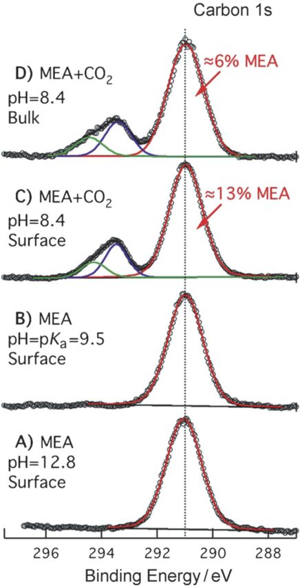
The Journal
                                                                                             PERSPECTIVE             scitation.org/journal/jcp
 of Chemical Physics

    Core level photoelectron spectroscopy
    of heterogeneous reactions at liquid–vapor
    interfaces: Current status, challenges,
    and prospects
    Cite as: J. Chem. Phys. 154, 060901 (2021); doi: 10.1063/5.0036178
    Submitted: 3 November 2020 • Accepted: 24 December 2020 •
    Published Online: 8 February 2021

    Rémi Dupuy,    Clemens Richter,                         Bernd Winter,    Gerard Meijer,       Robert Schlögl,
    and Hendrik Bluhma)

    AFFILIATIONS
    Fritz Haber Institute of the Max Planck Society, Faradayweg 4-6, D-14195 Berlin, Germany

    a)
         Author to whom correspondence should be addressed: bluhm@fhi-berlin.mpg.de

    ABSTRACT
    Liquid–vapor interfaces, particularly those between aqueous solutions and air, drive numerous important chemical and physical processes
    in the atmosphere and in the environment. X-ray photoelectron spectroscopy is an excellent method for the investigation of these interfaces
    due to its surface sensitivity, elemental and chemical specificity, and the possibility to obtain information on the depth distribution of solute
    and solvent species in the interfacial region. In this Perspective, we review the progress that was made in this field over the past decades
    and discuss the challenges that need to be overcome for investigations of heterogeneous reactions at liquid–vapor interfaces under close-to-
    realistic environmental conditions. We close with an outlook on where some of the most exciting and promising developments might lie in
    this field.
    © 2021 Author(s). All article content, except where otherwise noted, is licensed under a Creative Commons Attribution (CC BY) license
    (http://creativecommons.org/licenses/by/4.0/). https://doi.org/10.1063/5.0036178., s

    I. INTRODUCTION                                                            of pathogens and have recently attracted increased attention in
                                                                               connection with the spread of SARS-COV-2.4
          The liquid–vapor interface is of profound scientific, envi-                For a fundamental understanding of heterogeneous reactions
    ronmental, technological, and public health interest. The most             at liquid–vapor interfaces, experimental and theoretical techniques
    important liquid–vapor interface is arguably that between aqueous          are needed that are able to cope with the dynamic nature of the
    solutions and the surrounding air, which drives significant pro-           fluxional interface and provide information on its chemical com-
    cesses in the environment. One example is the uptake of CO2 at the         position and physical nature on the molecular scale. Investigations
    ocean–air interface, which has an estimated area of 3.6 × 10⁸ km2 .        of liquid–vapor interactions often require that the experiments are
    About one third of the anthropogenically generated CO2 is                  performed at elevated pressures, far away from ultra-high vacuum
    sequestered at this interface.1 Of similar importance are the uptake       conditions prevalent in traditional surface science studies. This is
    and release of trace gas molecules by aqueous aerosols, for instance,      particularly true for studies of aqueous interfaces at environmen-
    cloud and fog droplets, and the ensuing reactions. The estimated           tally relevant temperatures. Thus, the general challenges for experi-
    total volume of condensed water in the atmosphere2 is about                ments at liquid–vapor interfaces are similar to those in experiments
    1.3 × 10⁴ km3 ; assuming an average droplet diameter3 of 10 μm,            on solid–vapor interfaces, especially model studies of heterogeneous
    the total surface area of aqueous aerosols exceeds that of the oceans’     catalytic reactions. However, while investigations of solid–vapor
    by several orders of magnitude, emphasizing the importance of              interfaces have been pursued for a wide range of sample materi-
    aerosol heterogeneous chemistry for atmospheric and environmen-            als, structures, and reactions for many decades,5–8 there is a much
    tal processes. In addition, aerosols are involved in the transmission      smaller body of work for liquid–vapor interfaces. This is partly

J. Chem. Phys. 154, 060901 (2021); doi: 10.1063/5.0036178                                                                                  154, 060901-1
© Author(s) 2021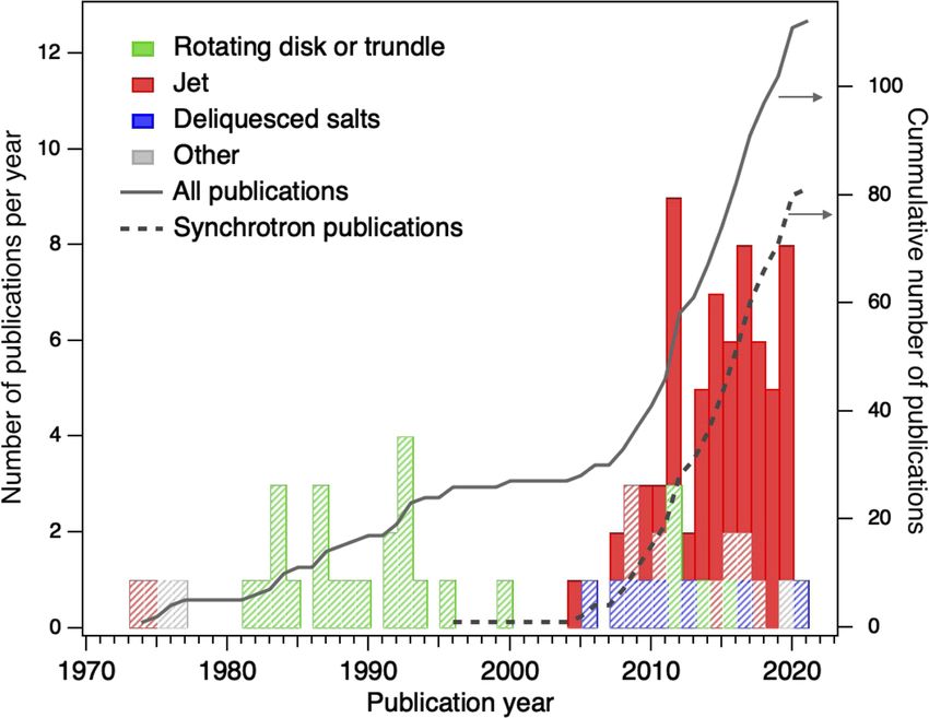
The Journal
                                                                                                          PERSPECTIVE             scitation.org/journal/jcp
 of Chemical Physics

    due to the difficulties posed by the preparation of well-controlled                      residing close to the liquid–vapor interface,11 contrary to earlier
    contamination-free model liquid–vapor interfaces and their investi-                      predictions from surface tension measurements12 and electrostatic
    gation with surface-sensitive probes.                                                    considerations13 that predicted that the interfacial region is devoid
         The scope of this Perspective is the application of core level                      of ions.
    photoelectron spectroscopy, which provides surface-sensitive ele-                              A wide variety of techniques has been used for surface-specific
    mental and chemical information, for the investigation of liquid–                        investigations of liquid–vapor interfaces. Historically, one of the
    vapor interfaces. We will review the development of the experimen-                       main characterization techniques has been the surface tension mea-
    tal capabilities over the past decades and give examples for new                         surement using the Wilhelmy method.14,15 This is essentially a
    developments in this field, including technical hurdles that need to                     macroscopic measurement that often requires modeling the effect
    be overcome for a more general applicability of core level photoelec-                    of solutes on the surface tension to provide information on quan-
    tron spectroscopy for studies of heterogeneous chemical reactions at                     tities such as the surface excess of molecules. These measure-
    liquid–vapor interfaces under realistic conditions.                                      ments can be combined with imaging methods such as Brewster
         Some of the chief scientific questions regarding liquid–vapor                       angle microscopy,16 which provides information on the homogene-
    interfaces concern (i) the chemical composition at the interface vs                      ity and 2D morphology of surfactant films on the sub-mm lengths
    the composition of the bulk liquid phase, (ii) the fundamental steps                     scale.
    during the uptake and release of trace gases, (iii) the formation and                          In the past 40 years, many more methods, a lot of which were
    the fate of reaction products at the interface and their potential                       adapted from solid-state surface science, have been applied to char-
    transport into the bulk phase, (iv) the role of surfactants, which can                   acterize liquid–vapor interfaces at the molecular level (see Ref. 17
    suppress or increase the interaction between gas phase and solution                      and references therein). Among these are linear and nonlinear
    species or participate in the reaction directly, and (v) the depen-                      optical vibrational spectroscopies:18 infrared reflection–absorption
    dence of these processes on conditions such as temperature, reactant                     spectroscopy (IRRAS,19–22 often called RAIRS in surface science23 ),
    velocity, reactant orientation, and the nature of the reactive chemical                  grazing angle Raman (GAR),18 vibrational sum-frequency genera-
    species (see Fig. 1).                                                                    tion (VSFG),24–26 and second-harmonic generation (SHG).26 These
         A wealth of information on the heterogeneous chemistry at                           techniques mainly provide information on the nature and orien-
    liquid–vapor interfaces has been obtained over the past decades                          tation of species at the interface and on the hydrogen-bonding
    using flow reactor studies, where aerosol droplets are exposed to                        network.
    reactive gases and the gas phase composition at the reactor outlet                             Another class of characterization methods are hard x-ray based
    is compared to that at the inlet.9,10 When the cumulative area of                        diffraction techniques.27,28 X-ray reflectivity27,28 (XR) probes the
    all aerosols in the reactor is known, quantitative information on                        electron density profile along the surface normal, which can be
    the uptake coefficients as well as reaction rates and products can                       interpreted in terms of molecular arrangements, depth distributions,
    be obtained. While these kinds of studies by their nature give an                        and surface roughness, while grazing incidence x-ray diffraction
    indirect view of interfacial reactions, they provided the first indi-                    (GIXD) and small angle scattering at grazing incidence28 (GISAXS)
    cations that some halide ions (such as I− and Br− ) are most likely                      probe also the in-plane properties of the surface and provide infor-
                                                                                             mation on surface ordering and molecular orientation. Resonant
                                                                                             variants of these techniques can achieve elemental specificity. An
                                                                                             additional x-ray based technique probing elemental composition
                                                                                             is x-ray fluorescence near total reflection27 (XFNTR), which is the
                                                                                             measurement slightly above and below the total reflection angle of
                                                                                             the (element-specific) x-ray fluorescence, giving bulk and surface-
                                                                                             sensitive information, respectively. Finally, surface X-ray Photon
                                                                                             Correlation Spectroscopy28 (XPCS) is used to dynamically probe
                                                                                             surface capillary waves through the analysis of an x-ray speckle
                                                                                             pattern.
                                                                                                   In the (mostly) soft x-ray range, x-ray absorption spectroscopy
                                                                                             (XAS) techniques have been used to probe unoccupied electronic
                                                                                             states of liquids and solutions in electron and fluorescent yield
                                                                                             modes.29–32 A particular focus of these studies has been on the
                                                                                             hydrogen-bonding network in water33,34 and the influence of the
      FIG. 1. Schematic representation of some of the fundamental processes that may         presence of solutes on it in aqueous solutions.32,35,36 A related
      occur at liquid–vapor interfaces. In this example, a vapor phase species X reacts      method is x-ray Raman spectroscopy,37 which, like the more recently
      with a rate constant k0 at time t0 with solution species to form a product Z0 at       used Resonant Inelastic X-ray Scattering (RIXS),38–40 was also
      the interface and possibly also a new vapor species Y0 . If Z0 is soluble, it will
      diffuse over time into the bulk. The different blue shading of the bulk and the sur-
                                                                                             employed to obtain specific information on the chemical nature and
      face region indicates that even in the absence of surface reactions, the chemical      environment of the probed atom, but since both methods rely on the
      composition of the interface region may be different from that of the bulk. The con-   detection of photons, they are less surface-sensitive.
      tinued reaction of the gas phase with the solution species can, over time, change            Ion scattering techniques have also been employed to study
      the chemical composition of the bulk and the surface region, as shown here in the      liquid–vapor interfaces.41,42 High energy (MeV or above) tech-
      vignette for t1 . This, in turn, may then change the nature of the surface and bulk    niques such as Rutherford Backscattering (RBS) or Elastic Recoil
      reactions.
                                                                                             Detection Analysis (ERDA) are less surface-sensitive due to their

J. Chem. Phys. 154, 060901 (2021); doi: 10.1063/5.0036178                                                                                               154, 060901-2
© Author(s) 2021
The Journal
                                                                                              PERSPECTIVE              scitation.org/journal/jcp
 of Chemical Physics

    high probing depth (typically 1 μm). However, their low-energy              conditions, which will not be covered here. The vapor pressure of
    (1 keV–10 keV) counterparts are used to investigate the inter-              water is about 6 mbar at the triple point and about 30 mbar at 25 ○ C.
    face. The detection of backscattered ions—low-energy ion scatter-           XPS measurements at these pressures require experimental strate-
    ing (LEIS), impact collision ion scattering spectroscopy (ICISS), or        gies that minimize the scattering of electrons by gas molecules, as
    direct recoil spectroscopy (DRS)—probes the elemental composi-              this otherwise leads to the attenuation of the detected photoelectron
    tion of the outermost layer. Detection of the 180○ backscattered            signal. There are two main approaches to overcome this obstacle:
    neutrals, as in neutral impact collision ion scattering spectroscopy        for one, the background pressure can be reduced by many orders
    (NICISS), has further utility since it can be used to obtain depth          of magnitude in experiments using fast flowing jets52 or droplet
    profiles of the chemical composition across the interface.                  trains,53 which are frozen out rapidly after the liquid jet was probed
          A related method is molecular beam scattering,43 which pro-           by XPS. This is a versatile approach for investigations of the interface
    vides information on the presence of solutes right at the interface,        chemical composition of solutions or for fast reactions, as discussed
    but perhaps even more important is a powerful method for the study          below.
    of heterogeneous reactions. Particles are typically detected using a              The other approach is used for studies of heterogeneous reac-
    quadrupole mass spectrometer, providing information on the nature           tions at liquid–vapor interfaces under steady-state conditions, where
    and velocity of the scattered molecules, but additionally, laser-based      the measurements are ideally performed in the presence of the equi-
    spectroscopic techniques can be applied to measure their rotational,        librium vapor pressure of the solution and the relevant trace gas
    vibrational, and electronic state populations.44 It is also an excellent    pressures, i.e., at elevated pressures. XPS can be adapted to opera-
    method to determine the interaction times between gas molecules             tion under non-vacuum conditions through the utilization of differ-
    and surface species and has been used to show that surfactants              ential pumping stages that reduce the path length of the electrons
    can both enhance and decrease the uptake of gas molecules at the            through the gas phase and thus, in turn, reduce scattering of the
    liquid–vapor interface.45                                                   electrons and signal attenuation. This adaptation of XPS, commonly
          Among electron spectroscopy techniques, metastable induced            named ambient pressure XPS (APXPS) or near-ambient pressure
    electron spectroscopy42 (MIES) is used to determine the valence             XPS (NAP-XPS), was developed first by the Siegbahn group in Upp-
    electronic structure [binding energy (BE)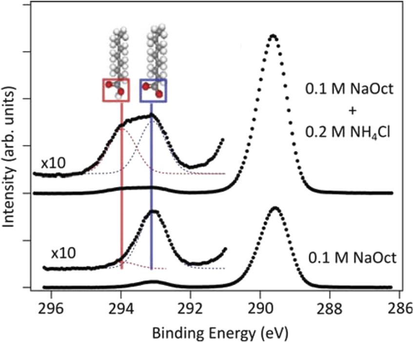
The Journal
                                                                                                                 PERSPECTIVE                  scitation.org/journal/jcp
 of Chemical Physics

      FIG. 2. Peer-reviewed original publications of XPS studies on liquid–vapor interfaces sorted by the preparation method for the liquid interface. Shaded areas indicate the
      fraction of studies that were performed in quasi-equilibrium, i.e., at the vapor pressure of the solution at the given temperature. Fully colored areas indicate studies where
      the background vapor pressure is strongly reduced through freezing-out of the solution after the XPS measurement. The solid line indicates the cumulative total number of
      publications over the past decades, starting from the first measurements at Uppsala University. The broken line shows the cumulative number of publications that resulted
      from experiments using synchrotron sources; these experiments have clearly gained importance over the past decade. This statistic only includes publications focusing on
      conventional XPS studies on core levels. Studies with particular focus on the valence electronic structure have been excluded as these deserve a separate review.

    TABLE I. Published XPS and APXPS investigations of liquid–vapor interfaces.a

    Solvent                                        Solute(s)                       Pressure (mbar)b             Equil.c          Year          Reference               Facility

    Liquid jet
    Formamide                          Pure, KI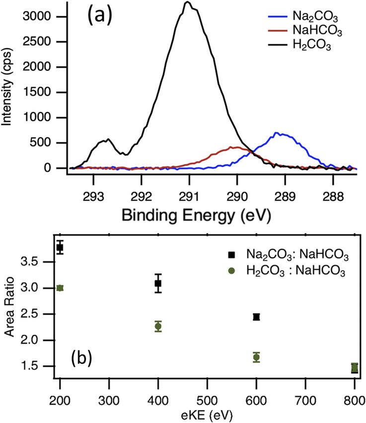
The Journal
PERSPECTIVE scitation.org/journal/jcp
of Chemical Physics
TABLE I. (Continued.)
Solvent Solute(s) Pressure (mbar)b Equil.c Year Reference Facility
Water H2 O2 10–4 No 2011 119 BESSY
Water Glycine NS No 2011 120 MAX-lab
Water Formic, acetic, butyric acid NS No 2011 121 MAX-lab
Water SiO2 nanoparticles (func.) NS No 2011 122 MAX-lab
Water HNO3 1.5 × 10⁻⁴ No 2011 123 BESSY
Water 10–4 No 2011 124 Spring-8
Water NaNO3 , HNO3 1.5 × 10⁻⁴ No 2011 125 BESSY
Water MEA, CO2 1.5 × 10⁻⁴ No 2011 126 BESSY
Water HCOOH 10–5 No 2012 127 BESSY
Water NaDecanoate, NaCl, Na2 SO4 , NS No 2012 128 MAX-lab
(NH4 )2 SO4 , NH4 Cl
Water, acetonitrile, LiI3 , LiI 10–5 No 2013 129 MAX-lab
ethanol
Water SiO2 nanoparticles 10–4 No 2013 130 BESSY
Water H2 SO4 10–4 No 2013 131 BESSY
Water NaCl, lysine 10–4 No 2013 132 Spring-8
Water 10–4 No 2013 133 BESSY
Water, acetonitrile 10−5 , 1.3 Both 2014 92 BESSY, ALS
Water HCOOH, NaCl 10–4 No 2014 134 SLS
Water KF, KCl, KBr NS No 2014 135 MAX-lab
Water Succinic acid NS No 2014 136 MAX-lab
Water GdmCl, NaCl, NH4 Cl NS No 2014 137 MAX-lab
Water NaCl, NaBr, NaI 10–4 No 2014 138 Spring-8, lab
Water NaCl NS No 2014 139 Spring-8
Water Trichloroethanol 10–5 No 2014 140 MAX-lab
Water, acetonitrile, LiI3 , LiI NS No 2015 141 MAX-lab
ethanol
Water K2 CO3 10−4 , 6 Both 2015 93 SLS
Water NaOctanoate, NaPropionate, NH4 Cl NS No 2015 142 MAX-lab
Water NaBr, citric acid 10–4 No 2015 143 SLS
Water TiCl3 10–4 No 2015 144 BESSY
Water 1-pentanol, 3-pentanol NS No 2015 145 MAX-lab
Water Alcohols (C1 –C4 ), carboxylic acids (C1 –C4 ) 10–4 No 2016 146 SLS
Water 1-butanol, tert-butanol, 1-pentanol, NS No 2016 147 MAX-lab
3-pentanol, 1-hexanol, 3-hexanol
Water Succinic acid, NaCl, NH4 Cl NS No 2016 148 MAX-lab
Water TiO2 nanoparticles, HNO3 1.3 Yes 2016 149 ALS
Water Alx Ox /SiO2 core–shell NPs 10–4 No 2016 150 SLS
Water HCOOH, Alx Ox /SiO2 core–shell NPs 10–4 No 2016 151 SLS
Water NaCl 10–4 No 2016 152 SLS
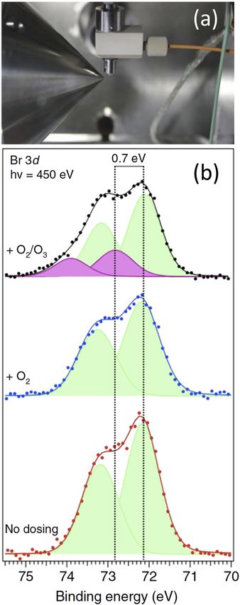
Water Br− , O3 10−3 –0.3 No 2017 153 SLS
Water [Co(CN)6 ]K3 10–4 No 2017 154 BESSY
Water Na2 CO3 , NaHCO3 , H2 CO3 10–2 No 2017 155 ALS
Water LiI, KI 1 Yes 2017 156 ALS
Water FeCl3 , NaOH 10–4 No 2017 157 BESSY
Water LiCl 10–4 No 2017 158 BESSY
Water Fe2 O3 nanoparticles 7.5 × 10⁻⁴ No 2018 159 BESSY
Water GdmCl, TPACl, Na2 SO4 , NaCl NS No 2018 160 MAX-lab
Water Hexylammonium chloride, NaHexanonate NS No 2018 161 MAX-lab
Water Butyric, pentanoic acid, butyl, hexyl NS No 2018 162 MAX-lab
amine, NaOH, HCl
Water NaCl, NaBr, NaI 10–4 No 2018 163 SLS
J. Chem. Phys. 154, 060901 (2021); doi: 10.1063/5.0036178 154, 060901-5
© Author(s) 2021
The Journal
                                                                                                   PERSPECTIVE          scitation.org/journal/jcp
 of Chemical Physics

    TABLE I. (Continued.)

    Solvent                                         Solute(s)                   Pressure (mbar)b     Equil.c     Year   Reference           Facility

    Water                           NaBr, NaI, 1-butanol, butyric acid                10–3             No        2019      164              SLS
    Water                           TiO2 NPs, HCl, HNO3 , NH4 OH                    3 × 10⁻³           No        2019      165             BESSY
    Water                           DMS, DMSO, DMSO2 , DMSO3                       1.5 × 10⁻⁴          No        2019      166             BESSY
    Water                           Carboxylic acids (C1 –C8 ), NH3                    NS              No        2019      167           MAX-lab
    Water                           Cysteine                                          10–4             No        2019      168         MAX-lab, LNLS
    Ammonia                         Pure                                            4 × 10⁻³           No        2019       60             BESSY
    Water                           NaI, TBAI, NH3 Cl                                  NS              No        2019      169          Spring-8, lab
    Water                           H2 SO4 , FeSO4                                  5 × 10⁻⁴           No        2019      170          Lab (irvine)
    Ammonia                         KI, NH4 I                                         10–3             No        2020       61             BESSY
    Ammonia                         Li, Na, K                                         10–3             No        2020       62             BESSY
    Droplet train
    Water                           Methanol                                           5              Yes        2008       53                ALS
    Moving wire
    Ethylene glycol                                                                   10–1            Yes        1975      171          Lab (Uppsala)
    Ethylene glycol                 N-methyl-glucamine salts                           NS             Yes        1976      172          Lab (Uppsala)
    Rotating trundle
    Ethanol, methanol               NaI, I2                                           NS              Yes        1981      173          Lab (Uppsala)
    Formamide                       Pure                                                              Yes        1982      174          Lab (Uppsala)
    Glycol                          Ag+ , Cu+ , Zn2+                                  NS              Yes        1983      175          Lab (Uppsala)
    Glycol                          Na+ , K+ , Rb+ , Cs+                              NS              Yes        1983      176          Lab (Uppsala)
    Ethanol                         NaI, I2                                           NS              Yes        1983      177          Lab (Uppsala)
    Glycol, ethanol                 Mg2+ , Ca2+ , Sr.2+ , Ba2+ , Ag+ , Zn2+ ,         NS              Yes        1984      178          Lab (Uppsala)
                                    Cd2+ , Hg2+ , Mn2+
    Glycol                          F− , Cl− , Br− , I− , I2 , I−3 , NO−3             NS              Yes        1984      179          Lab (Uppsala)
    Water                           LiCl, glycol, dimethylformamide                  0.1–1            Yes        1986      180          Lab (Uppsala)
    Tetramethyl guanidine           NaI, water                                        NS              Yes        1986      181          Lab (Uppsala)
    Formamide                       TBAI                                              NS              Yes        1986      182          Lab (Uppsala)
    Formamide                       Octanol, bromooctanol                          4 × 10⁻²           Yes        1987      183          Lab (Uppsala)
    Formamide                       Tetra-N-alkylammonium salts                       NS              Yes        1988      184          Lab (Uppsala)
    Heptane                         Butyllithium                                      NS              Yes        1989      185          Lab (Uppsala)
    Glycol                          NaOH, Be2+                                        NS              Yes        1992      186          Lab (Uppsala)
    Rotating disk
    Formamide                       TBA salts, (IPrNBu3 )I                            NS              Yes        1991      187          Lab (Uppsala)
    Formamide                       Potassium octanoate, potassium                    NS              Yes        1991      188          Lab (Uppsala)
                                    11-bromoundecanoate
    Formamide, ethylene             Potassium octanoate                               NS              Yes        1992      189          Lab (Uppsala)
    glycol
    Formamide                       TBABr, Tributyl(bromomethyl)NBr,                  NS              Yes        1992      190          Lab (Uppsala)
                                    NH4 Cl
    Formamide                       TBABr, TBPBr                                      NS              Yes        1992      191          Lab (Uppsala)
    Formamide, ethylene             Potassium octanoate                               NS              Yes        1993      192          Lab (Uppsala)
    glycol
    Formamide                       CsI, TBANO3 , potassium octanoate                 NS              Yes        1995      193          Lab (Uppsala)
    Formamide                       CsI, TBANO3                                       NS              Yes        1999      194          Lab (Uppsala)
    Formamide                       TBACl                                             NS              Yes        2010      195           Lab (leipzig)
    Formamide                       TBPBr                                             NS              Yes        2011      196           Lab (leipzig)
    Formamide                       TBAI                                              NS              Yes        2011      197           Lab (leipzig)
    Formamide                       TBAI                                              NS              Yes        2011      198           Lab (leipzig)
    HPN                             POPC, TBABr                                       NS              Yes        2013      199           Lab (leipzig)

J. Chem. Phys. 154, 060901 (2021); doi: 10.1063/5.0036178                                                                                     154, 060901-6
© Author(s) 2021
The Journal
                                                                                                                 PERSPECTIVE                  scitation.org/journal/jcp
 of Chemical Physics

    TABLE I. (Continued.)

    Solvent                                    Solute(s)                   Pressure (mbar)b                 Equil.c             Year              Reference                Facility

    Liquid lamella
    Formamide                            TBAI                                      10–4                       No                1995                   94                  BESSY
    Static droplet
    Propylene carbonate                  LiClO4                                 2 × 10⁻¹                      Yes               2015                 200                  MAX-lab
    Propylene carbonate                  LiTFSI                                 2 × 10⁻¹                      Yes               2019                 201                  MAX-lab
    Deliquesced salt
    Water                                KBr, KI                                    2                         Yes               2005                 202                   ALS
    Water                                KI, butanol                                2                         Yes               2007                 203                   ALS
    Water                                NaCl, Br                                   2                         Yes               2008                 204                   ALS
    Water                                NaCl, NaClO4                               5                         Yes               2009                 205                   ALS
    Water                                NaCl                                     0.1–1                       Yes               2010                 206                   ALS
    Water                                NaCl, RbCl, RbBr                           5                         Yes               2012                 207                   ALS
    Water                                NaCl, NaBr, NaI                            8                         Yes               2015                 208                  SOLEIL
    Water                                NaCl, NaI                                  8                         Yes               2016                 209                  SOLEIL
    Water                                NaAcetate                                 0.7                        Yes               2020                 210                    SLS
    a
      Included in this table are all APXPS papers on liquid–vapor interfaces that we know of, as of May 2020. To keep the scope of this table to a reasonable size, we exclude studies
    performed at background pressures lower than 10−5 mbar (most notably, XPS studies of ionic liquids or pre-melted liquids) and studies focusing mostly on resonant/Auger emission
    spectroscopy or valence band PES (binding energies
The Journal
                                                                                             PERSPECTIVE                scitation.org/journal/jcp
 of Chemical Physics

    identified. Moreover, the so-called chemical shifts within each core       B. Relevant time scales for liquid–vapor interface
    level spectrum allow for distinguishing different chemical species of      reactions
    an element (e.g., oxidation states and functional groups). The strong            Chemical reactions take place over a multitude of time scales
    dependence of the probing depth in XPS on the electron kinetic             from electron transfer and bond-breaking/making events on ultra-
    energy allows us to obtain depth-dependent information on the ele-         fast time scales to much slower changes in the conformation of
    mental and chemical composition at an interface. Typical probing           larger molecules. Here, we are interested in the time that it takes
    depths are in the nanometer range. Changes in the work function            to reach a steady-state at the liquid–vapor interface and in the bulk
    or potential at the surface can also be detected since these affect the    solution upon a change in the gas phase composition, which is rele-
    electron kinetic energy in all core levels and valence spectra and can     vant for the investigation of heterogeneous reactions at liquid–vapor
    thereby be distinguished from chemical shifts. Moreover, through           interfaces.
    the measurement of the low kinetic energy cutoff, the absolute value             Let us consider the simple situation of an aerosol droplet with
    of the work function of the sample can be determined; while this           a characteristic diameter d of 10 μm consisting of pure water in the
    method has been applied in investigations on solid samples, it has         absence of any surfactants. Let us assume that initially, the droplet
    yet to be demonstrated for liquids.                                        is in equilibrium with its vapor (i.e., neither growing nor shrink-
          As we have pointed out before, for investigations of heteroge-       ing). The droplet is then suddenly exposed to the atmospheric CO2
    neous reactions at aqueous solutions, it is, in most cases, necessary      partial pressure of 0.4 mbar. What is the time scale for equilibrat-
    to perform measurements at pressures in the mbar range. The mean           ing the liquid–vapor interface upon the jump in CO2 partial pres-
    free path of electrons in the gas phase at these pressures is strongly     sure, and how long will it take for the bulk to reach a steady-state
    reduced due to inelastic scattering by gas molecules. A simple esti-       concentration of CO2 ?
    mate for water vapor shows that, since the density of water vapor                Let us first neglect chemical reactions occurring in liquid water.
    at 1 mbar is about 10−6 of that of condensed water, the mean free          Schwartz and Freiberg76 and Shi and Seinfeld77 calculated the char-
    path of electrons is about 106 of that in the solution, i.e., is in the    acteristic time scale τ da at which the equilibration of the bulk
    mm range. The path length of the electrons through the gas phase           solution proceeds,
    thus has to be limited to about an mm (or even less when work-
    ing at higher pressures), which can be achieved using a differentially                                             d2
    pumped aperture between the sample cell and the electrostatic lens                                      τda =                 ,                   (1)
                                                                                                                    π2 D    sol
    system of the electron spectrometer. Typical pressure differentials
    across these apertures are 10−2 to 10−4 . Several differential pump-
    ing stages are necessary for sample cell pressures in the mbar range       with Dsol being the diffusion coefficient in the solution, which is
    to ensure high vacuum conditions and avoid arcing at the electron          2 × 10⁻⁹ m2 /s for our example of CO2 in water at room temper-
    detector, which is operated at high voltages. These ambient pressure       ature.78 For a 10 μm droplet, this then gives an equilibration time
    XPS spectrometers are now commercially available and have been             of about 5 ms, which is on the order of the time scales available in
    installed in many laboratories and synchrotron facilities around the       droplet train79,80 and liquid jet experiments (see below).
    world. For more detailed information on APXPS, we refer the reader               Since XPS is sensitive only to the interfacial region, the equi-
    to a number of review articles (among them, Refs. 69–75).                  libration time for the bulk is not necessarily the most important
          The close proximity of the sample surface to the differentially      parameter in these experiments. A characteristic time scale τ pp for
    pumped front aperture of the electrostatic lens system of the electron     the establishment of an equilibrium at the liquid–vapor interface
    analyzer can disturb the gas flow and local pressures at the sam-          can be calculated, again without accounting for chemical reactions,
    ple surface, which needs to be evaluated to ensure that the pressure       according to Seinfeld,81 as
    and flow gradients do not interfere with the experiment. In addi-
    tion, the distance between the sample surface and the aperture has                                                 4HRT 2
    to be as constant as possible; otherwise, the photoelectron intensity                               τpp = Dsol (        ),                        (2)
                                                                                                                        αv̄
    fluctuates strongly due to the exponential dependence of the elec-
    tron attenuation on the distance that the electrons travel through the
    gas. Both of these considerations are usually not relevant in experi-      with H being Henry’s law constant, R being the gas constant, T
    ments on solid samples but pose a serious challenge to experiments         being the temperature, α being the mass accommodation coefficient,
    on liquids, where slight variations in the surface position on the         and v̄ being the average velocity of the molecules in the gas phase.
    0.1 mm scale can not only lead to signal fluctuations but also, in the     Using numbers for the CO2 –water system at room temperature, i.e.,
    worst case, to entering of the liquid into the electrostatic lens system   T = 298 K, H = 3.4 × 10⁻² mol l−1 atm−1 ,82,83 α = 2 × 10⁻⁴ ,3 and
    through the front aperture, with potentially dire consequences for         v̄ = 380 m/s, one arrives at equilibration times for the interface in
    the components of the lens system, including electrical shorts and         the μs range, i.e., several orders of magnitude faster than required in
    corrosion. The preparation of liquid surfaces for XPS and APXPS            bulk solution.
    experiments is thus a challenge in itself.                                       The equilibration timescales derived above, which do not con-
          Before discussing strategies for the preparation of liquid–vapor     sider chemical reactions, can, however, be much shorter than the
    interfaces for surface-sensitive investigations, we first consider the     time required to reach chemical equilibrium. In the widely studied
    relevant time scales for reactions at liquid–vapor interfaces, since       case of CO2 dissolution,84 CO2 reacts with either H2 O or OH− (the
    these often govern the choice of preparation method for a given            latter reaction dominates for pH > 8.5) to form carbonate species,
    investigation.                                                             which are themselves in an acid–base equilibrium depending on

J. Chem. Phys. 154, 060901 (2021); doi: 10.1063/5.0036178                                                                                     154, 060901-8
© Author(s) 2021
The Journal
                                                                                               PERSPECTIVE                  scitation.org/journal/jcp
 of Chemical Physics

    the pH. The abundance of these different species and equilibration
    timescales involved in the reactions are governed by the kinetic con-
    stants of this reaction network and the composition of the aqueous
    solution. The equilibrium values and kinetic constants depend on
    the pH, temperature, and pressure,85–87 and the equilibrium is also
    influenced by the presence of other ions and molecules, which affects
    the activities of the species in the carbonate system. The timescale
    for equilibration of a closed and homogeneous aqueous carbon-
    ate system at room temperature can be estimated84 to be of the
    order of minutes, depending on the pH and CO2 concentrations.
    For an open system where also gas–liquid exchanges are considered,
    equilibration can take even longer. Diffusion is also not accounted
    for in this estimation: for a small system such as the droplet case
    developed above, we saw that the physical timescale of equilibration
    driven by gas–liquid exchanges and bulk diffusion is much smaller           FIG. 3. Equilibration time of a sodium-dodecylnapthalene-sulfonate (SDNS) sur-
    than the chemical equilibration timescale. On the other hand, for           factant layer on water. Open circles show the surface pressure measured by the
    larger systems, Eq. (1) shows that the physical timescale can become        Wilhelmy method, while full circles display the change in nonlinear susceptibility
    much larger than the chemical one. The coupling of the reaction and         χ m /χ 0 obtained from a second-harmonic measurement. The line is a Langmuir-
    diffusion is specifically treated in Ref. 84.                               type fit of the surface coverage by SDNS. Reprinted with permission from Rasing
                                                                                et al., J. Chem. Phys. 89, 3386 (1988). Copyright 1988 AIP Publishing LLC.
          The equilibration timescale of the interface taking into account
    chemical reactions is difficult to estimate, and in fact, the investiga-
    tion of the relations between the bulk and the surface composition
    and reactivity represents an excellent example for the application of
    liquid interface science.
          While the physical equilibrium between small gas molecules           10−6 mbar, differential pumping between the experimental chamber
    and the aqueous solution surface is established at short timescales,       and analyzer is necessary, and for experiments at pressures above
    the situation is different when we consider the presence of sur-           0.1 mbar, several differential pumping stages and very short path
    factants at the interface. Depending on the size of the surfactant         lengths of the electrons inside the experimental cell are required
    molecule, the kinetics of the adsorption of these molecules to the         to reduce scattering of electrons by gas molecules, as described in
    surface from the bulk can be on the scale of many minutes or               Sec. II A.
    even hours. This has been shown by Rasing et al.88 in Langmuir                   Figure 4 shows different preparation methods, most of which
    trough measurements for the case of sodium-dodecylnapthalene-              have already been used for XPS experiments on liquid–vapor inter-
    sulfonate (SDNS). In these measurements, the SDNS surfactant was           faces. The methods in the upper row of Fig. 4 rely on fast flow-
    dissolved into water and the surface of the trough was disturbed           ing liquids that are injected into the vacuum chamber and propa-
    using one of the barriers, driving some of the SDNS molecules into         gate through it at considerable speed; typical flow rates for jets and
    the bulk. After separating the two barriers again, the re-adsorption       droplet trains are of the order of many tens of m/s. If the liquid is
    of SDNS to the water–vapor interface was monitored through sur-            caught in a (LN2 ) cooled trap, the background pressure in the vac-
    face pressure measurements using the Wilhelmy method, as well              uum chamber can be kept in the high vacuum region, for instance,
    as SHG.                                                                    below 10−4 mbar for water that is injected at room temperature
          The results are shown in Fig. 3. The change in the nonlin-           into the chamber. This enables XPS experiments with very good
    ear susceptibility χ m /χ 0 and the surface pressure with time is in       signal-to-noise ratios and only minimal requirements for additional
    good agreement and can be modeled with a Langmuir adsorption               differential pumping. These methods have been used in the past to
    isotherm. The data in Fig. 3 show that it takes more than an hour          investigate the properties of the chemical composition of solutions,
    until the surface reaches a steady-state condition.                        where the fast flowing jet or droplet train reduces or even eliminates
          The examples above demonstrate that the equilibration of the         the commonly encountered problems of beam damage and surface
    interface proceeds on a wide range of time scales, depending on the        contamination.
    species involved. In the following, we discuss some of the approaches            The fast flowing jet52 or droplet80 setups allow for the change
    for the preparation of liquid–vapor interfaces, which are suitable for     in the solution concentration or pH quickly and seamlessly since
    XPS and APXPS experiments.                                                 the source of the solution is kept outside of the vacuum chamber.
                                                                               Jet and droplet sources can also run in fast mixing modes, where
                                                                               two solutions of different chemical compositions are either mixed
    C. Preparation of liquid surfaces for XPS                                  just before entering the measurement chamber or mixed inside
         There are a number of different methods for the prepara-              the chamber (colliding jet/droplet);89–91 the latter mixing scheme
    tion of liquid interfaces for XPS experiments. The choice of the           enables measurements from time zero of the mixing event. These
    appropriate method depends on the goal of the experiment and               methods, in general, provide opportunities for time-resolved stud-
    the thermodynamic conditions, particularly the vapor pressure of           ies on the sub-ms to ms time scales for nucleation events and the
    the solution at the desired sample temperature, as well as the time        study of short-lived reaction intermediates. This is especially true
    scale of the expected reactions. For experiments at pressures above        for droplet trains, which, in principle, offer a longer time scale for

J. Chem. Phys. 154, 060901 (2021); doi: 10.1063/5.0036178                                                                                             154, 060901-9
© Author(s) 2021
The Journal
PERSPECTIVE scitation.org/journal/jcp
of Chemical Physics
FIG. 4. Preparation of liquid–vapor interfaces inside vacuum chambers. The upper row shows methods based on fast moving jets or droplets that have a very brief interaction
time with the surrounding environment before being measured. These methods can be used in a vacuum environment since the liquid reservoir is outside of the vacuum
chamber. The bottom row shows preparation methods where the bulk reservoir of the liquid is inside the vacuum chamber and the measurements thus are done in the
presence of the equilibrium vapor pressure. These investigations permit longer interaction times between gases and the liquid.
the investigations, since droplets are stable for many centimeters of makes these methods very attractive, though, is that the liquid sur-
travel, while jets break up after a few mm due to Rayleigh instabili- face being measured is constantly refreshed (albeit at a slower rate
ties. Another feature of fast-flowing jets or droplet trains is the fast that in a liquid jet) and thus not very prone to x-ray induced beam
evaporation (when used in conjunction with a LN2 trap), which con- damage.
tinually decreases the temperature along the propagation direction, For experiments with (in theory) unlimited reaction times,
which can be used as an additional parameter in an experiment if the static liquid surfaces can be prepared in a number of ways, which
temperature drop can be calibrated, but also, by definition, creates a are depicted in the right part of the bottom row of Fig. 4. Common
non-equilibrium at the liquid–vapor interface. Operating a liquid jet to all of these methods is that the measurements have to be done in
under equilibrium vapor pressure conditions nonetheless can and the presence of the equilibrium vapor pressure of the solution; oth-
has been done.92,93 erwise, the sample will evaporate during the measurements. Hence,
Many environmental processes occur over longer time inter- these preparation methods require APXPS measurements for most
vals than ms and thus require approaches with a longer exposure of the solutions of interest, chiefly those of aqueous nature. The most
time between the liquid and the gas phase. Three of those, based on straightforward way is to deposit a droplet of the solution onto a
the wetting of a solid substrate in a continuous manner, are shown non-reactive substrate, either before evacuation of the chamber or
in the left part of the bottom row of Fig. 4. The rotating disk (or after, in the latter case, e.g., through the use of a pulsed valve. Depo-
trundle), wetted wire,67 and liquid lamella94 methods can be used for sition onto a substrate can also be done through condensation from
intermediate time scales between the fast flowing jets and truly static the vapor phase. This works well for pure solvents, without the addi-
methods. One point to keep in mind with these approaches is that tion of a solute, which will not readily evaporate and adsorb on the
the reservoir from which the wetting film is created is also in contact substrate.
with the gas phase, i.e., there is always, most likely, a convolution Another straightforward method to investigate saturated aque-
between the reaction proceeding on the liquid–vapor interface of the ous solutions is to deliquesce a salt by adjusting the relative humidity
wetted surface that is measured by XPS and the reaction between the in the measurement cell to the appropriate value, which, for most
liquid in the reservoir and the gas atmosphere in the measurement alkali halides, is between 20% and 90%.95 The deliquescence point is
chamber. This also means that the background vapor pressure is set a triple point in the phase diagram of salts and water vapor, with
by the equilibrium vapor pressure of the solution in the reservoir, the solid salt, water vapor, and the saturated solution in equilib-
which can be temperature-controlled and thus adjusted over some rium with each other. While the concentration of the solution is thus
range down to that of the pressure close to the freezing point. What well known, the downside of this method is that it does not permit
J. Chem. Phys. 154, 060901 (2021); doi: 10.1063/5.0036178 154, 060901-10
© Author(s) 2021The Journal
PERSPECTIVE scitation.org/journal/jcp
of Chemical Physics
the change in the concentration of the solution in a controlled way. incident photon energy hν reveals the binding energy (BE) of a
Only after all of the solid salt is deliquesced will the concentration given element and orbital through the relation BE = hν − KE.
of the solution decrease; however, not in an easily adjustable way. The core level BE also depends on the local chemical environ-
One advantage of this method, on the other hand, is that it deliv- ment (observable through the so-called “chemical shifts”)5,47 and
ers reliable sensitivity factors for the quantification of relative ionic thus serves as a reporter of structural details, including the pro-
concentrations through the measurement of the dry salt at low RH tonation state in aqueous solutions.111,121,162 It is, hence, common
before the sample is deliquesced. to present measured photoelectron spectra on the BE scale, even
The other two methods that allow, in principle, unlimited reac- though the measured quantity is the KE. Conversion of KEs to BEs
tion times are the so-called dip-and-pull (or meniscus) technique requires a reference point for the BE scale, for instance, the vac-
and Langmuir troughs. The dip-and-pull method is currently being uum level or the Fermi edge, or, in some cases, the BE of a certain
used for APXPS measurements of solid–liquid interfaces,96–99 since core level, as will be discussed below. The underlying model for
it allows the preparation of ultra-thin (10 nm–20 nm) solution films the calculation of the BE values needs to be clearly stated so that
on solid substrates by slowly pulling out the substrate from the bulk the measured KE values can be retrieved for comparison with other
solution in the presence of the saturation vapor pressure, akin to the measurements.
procedure used in a Langmuir–Blodgett process. The measurement In most cases, the electron spectrum contains contributions
position is usually many mm (or even cm) above the bulk liquid level in addition to photoelectrons, for instance, from electrons emit-
in the reservoir, leading to potential limitations in the electronic and ted in second-order relaxation processes (such as Auger decay or
ionic transport along the ultra-thin liquid film. Measurements can other autoionization pathways47,211–214 ) or electrons that have lost
be done over many hours as long as the liquid film is stable. This discrete or non-discrete fractions of their initial KE through inelas-
method naturally also lends itself to investigations of liquid–vapor tic scattering. Presenting those contributions on the same BE scale is
interfaces. rather meaningless, although commonly accepted within the com-
The last method discussed here is Langmuir troughs, which munity; the correct presentation is the measured KE, which, how-
have, for many decades, been used for the investigation of the ever, is inconvenient when addressing orbital energies. For the sake
physico–chemical properties of surfactant layers.100,101 In a Lang- of completeness, we would like to mention that further complica-
muir trough setup, movable barriers allow us to dynamically adjust tions arise when the core level photoemission spectra are measured
the packing density of the surfactants and thus to investigate near the ionization threshold, the case in which the direct photoelec-
their influence on the structure and chemistry at the liquid–vapor tron and the Auger electron exchange energy via Coulomb interac-
interface. Traditionally, surface-sensitive measurements on thus- tion with the remaining 1+ and subsequently 2+ charged (final state)
prepared surfactant films were performed using optical spectroscopy ionic species. This so-called post collision interaction (PCI) can be
and hard x-ray based scattering techniques. Some of the authors of detected as a distortion and shift of both direct and secondary elec-
this Perspective have recently demonstrated that APXPS is a suit- tron peaks.215–217 For water and aqueous solutions, PCI studies have
able method for the investigation of the vapor–surfactant/aqueous not yet been reported though.
solution interface and can provide complementary information to Another important issue regarding measured electron energies
optical and scattering methods.102 We discuss the opportunities for from water or aqueous solutions is the determination of the abso-
combined APXPS/Langmuir trough measurements in the last part lute value of a given BE, which requires a robust reference point for
of this Perspective. the energy scale. Neat water is electrically non-conductive (water
Table I lists—to the best of our knowledge—all XPS and APXPS can be regarded as a wide-bandgap semiconductor218 ), whereas
measurements on liquid–vapor interfaces that have been published electric conductivity in the case of dispersed ions can be large.
by the end of May 2020. This table is organized with the preparation Hence, for neat water as well as in poorly conductive aqueous solu-
method for the liquid–vapor interfaces and lists solvents/solutes as tions, the KE of the measured photoelectrons depends on a num-
well as background pressures in the experiments. From the table, it ber of charging effects of the liquid surface (including electrokinetic
is obvious that the overwhelming number of experiments have been charging in the case of fast flowing liquid samples and radiation-
performed so far under vacuum conditions using the liquid micro- induced charging219 ), which are typically difficult to quantify
jet technique, while investigations under equilibrium vapor pressure experimentally.
conditions are in the minority so far. In general, the use of gas phase vapor peaks as the internal
After discussing the preparation methods for liquid–vapor binding energy reference requires a careful evaluation of the experi-
interfaces, we now proceed to consider some of the distinct aspects mental conditions. The vacuum level of the gas phase is tied to that
of the analysis of XPS data measured at those interfaces, which can, of the nearest surfaces, here chiefly the liquid–vapor interface (in
in some cases, vary with regard to the more commonly obtained data APXPS measurements also, the front aperture of the differentially
on solid interfaces. In the following, we focus on the basic quantities pumped electrostatic lens system). Any change in the position of
in an XPS experiment, the signal intensity and electron energy. We the vacuum level of the interface, be it through streaming potentials
start with the non-trivial matter of referencing the electron binding at the nozzle of liquid jet apertures, through partial orientation of
energy scale. dipoles at the interface, or the preferential presence of certain ions at
the interface, will have an influence on the measured gas phase KE.
If it can be assured that no electric fields exist between the solution
D. Energy referencing
surface and electron detector, solute and solvent peaks can be rea-
One of the quantities measured in an XPS experiment is the sonably well calibrated with reference to the known binding energies
kinetic energy (KE) of the ejected photoelectrons, which for a known of gas-phase water.
J. Chem. Phys. 154, 060901 (2021); doi: 10.1063/5.0036178 154, 060901-11
© Author(s) 2021The Journal
PERSPECTIVE scitation.org/journal/jcp
of Chemical Physics
Commonly used references in the literature are the O 1s BE the incident photon flux, which is implicitly assumed to be constant
or the 1b1 BE of neat liquid water, which, however, have them- throughout the probed volume in this formula, since the penetra-
selves been determined by reference to the respective gas phase water tion depth of x rays is much larger than the probing depth of XPS.
orbitals BEs.52,109 Furthermore, the BE of these orbitals of water dσ
dΩ
is the differential photoemission cross section of the element at
might themselves depend on the presence of solutes and their con- the given photon energy, which represents the probability of emis-
centrations and thus not be a meaningful reference. On the contrary, sion of a photoelectron in the direction of the spectrometer, and thus
a BE shift of the core and valence levels of water as a function of the also depends on the experimental geometry. It can be further bro-
solute type and concentration is in itself a quantity that can con- ken down as dΩ dσ
= σfσ (θ, ϕ), where σ is the integrated cross section
tain valuable information. This information is lost if the BEs of these and fσ is a function describing the electron emission anisotropy. T
peaks are used as an internal reference and set to a certain fixed is the transmission function of the spectrometer, which depends on
value. the kinetic energy of the photoelectron. The last term is the integral
Different approaches that bypass the gas-phase reference are over the probed volume of the density N of the considered element
pursued at present, exploiting the information contained in the low- at a given point multiplied by an attenuation factor F. Attenuation
energy cutoff of the photoelectron spectra. The principal idea has of the signal is characterized by the mean escape depth (MED) of
been outlined by Tissot et al. for highly saturated salt aqueous solu- the electrons, which itself primarily depends on their inelastic mean
tions deposited on a gold substrate.208 The analysis here is based free paths (IMFPs, see Sec. II E 2). F therefore depends on the photo-
on a condensed-matter description, specifically the determination electron kinetic energy and the composition and thickness of all the
of the Fermi energy and work function. This challenging approach material between the emission point and the entrance of the electron
is promising for liquid samples with a high electrical conductivity energy analyzer, including the gas phase, which can be relevant for
but suffers from the same limitations in the case of low-conductivity applications at relatively high pressures.
liquids as one encounters in XPS investigations on oxides with high For most practical uses, F is written in the following way:
bandgaps.
The ability to measure the work function of the solution surface
z
in vacuum, where possible, will provide valuable additional infor- F(z, eKE) = exp(− ), (4)
mation in XPS spectra acquired on liquid interfaces, allowing us λ(eKE)cos(θ)
to quantify the presence and net orientation of molecular surface
dipoles. where θ is the detection angle of the electrons relative to the surface
normal and λ is either directly the IMFP for the considered envi-
E. Quantification and depth-profiling ronment [in the so-called straight-line approximation (SLA) and
for a flat surface] or an effective attenuation length (EAL) that also
For a better understanding of heterogeneous chemical reactions takes into account elastic scattering and geometrical factors (see
between aerosols and the surrounding gas phase, quantitative infor- Secs. II E 2–II E 4).
mation on the chemical composition of the liquid–vapor interface is Liquid–vapor interfaces are not as sharp as solid–gas interfaces,
essential to aid in the development of atmospheric models. XPS is although they exhibit a steep pressure gradient. The broader width
a quantitative technique particularly suited for this purpose and has of the interfacial region and the often steep gradients in the con-
been extensively used in solid state surface science. Detailed tuto- centration of ions as a function of depth affect the calculation of the
rials on quantification in the solid state exist in textbooks47,220,221 effective attenuation, for which a step-like model for the interface [as
and will not be reiterated here. Instead, we focus on the most in Eq. (4)] is hence not appropriate. Following the work of Ottosson
important aspects with regard to liquid interfaces and present some et al.,117 a better description of the attenuation can be achieved by
experimental strategies for quantification. A broader question con- integrating over the density profile at the interface,
cerns the determination of concentration depth profiles of species
across the liquid–vapor interface. This leads us to discuss also the z N(z)
F ′ (z, eKE) = exp(−
1
depth sensitivity of XPS, different depth-profiling techniques, and
λ(eKE)cos(θ) ∫0 N∞
dz), (5)
the use of photoelectron angular distributions (PADs) to address this
problem.
with N∞ and N(z) being the total densities of the bulk and at depth
1. Quantification z, respectively. λ is assumed here to represent the IMFP for the
bulk.
The expression for the measured XPS signal intensity for a
In a strict sense, the attenuation depends not only on the depth-
given peak is usually written in the following form,117,220 which
dependent total density but also on the depth-dependent composi-
breaks down the different factors that need to be considered in the
tion of the interface. This is more complicated to take into account
quantification of XPS data:
and also depends on the a priori knowledge of the partial den-
sity depth profiles of all different species in the solution, which is
dσ usually the unknown quantity that one tries to discern in an XPS
I = αΦ(hν) (hν)T(eKE) ∫ N(⃗r)F(eKE,⃗r)dV, (3)
dΩ experiment.
Quantification, in general, aims at the determination of the
where α is a geometrical factor depending on the illuminated area of depth-dependent density N(z) of an element of a species of inter-
the sample and the angular acceptance of the electron analyzer. Φ is est. If using Eq. (3), the fundamental quantities involved (Φ, σ, D,
J. Chem. Phys. 154, 060901 (2021); doi: 10.1063/5.0036178 154, 060901-12
© Author(s) 2021The Journal
PERSPECTIVE scitation.org/journal/jcp
of Chemical Physics
IMFPs, etc.) need to be known, or experimental strategies have to produce photoelectrons of the same kinetic energy when ionizing
be used where these quantities can be eliminated, for instance, by different orbitals or different elements. This eliminates the T fac-
measuring relative chemical compositions. In many cases, approxi- tor as well as some of the factors arising from the kinetic energy
mations are required due to the lack of information on the absolute dependence of electron mean free paths, leaving the photon flux and
values of some of the experimental parameters. cross sections as the only unknown factors. When experiments are
Some related specific points that go beyond the problem of performed at constant photon energy, one can perform calibration
quantification are discussed in separate sections afterward but are experiments on a well-known gas (e.g., CO2 for the C/O ratio) to
mentioned here already briefly since they are relevant for the discus- obtain a calibration for both the T factor and the photoemission
sion of the quantification: cross section σ. It is also convenient when possible to only compare
signal intensities of the same element (e.g., carbon) to eliminate most
● Inelastic mean free paths are the fundamental quantities that factors from the equation. For example, although it requires some
set the depth sensitivity of XPS, but also one of the biggest simplifying assumptions, some authors128,136 have used ions known
unknowns. The relation between the attenuation factor and to be depleted at the surface as a bulk reference to separate bulk and
IMFP depends on the experimental geometry, but also on surface contributions from the signal of other similar species (e.g.,
elastic scattering, which cannot always be neglected. These succinic acid and its fully deprotonated form136 ).
points are discussed in Sec. II E 2. In some cases, provided that all the above mentioned quanti-
● The qualitative and quantitative investigation of surface ties can be estimated or cancel out, Eq. (3) can be used to obtain
enhancement/depletion of certain species and the general the density of a species by a simple calculation. In solid state studies,
problem of retrieving the full density profile N(z) of a given this is commonly done for layered structures or homogeneous alloys,
species can be addressed using depth-profiling experiments, i.e., when the density can be assumed to be constant over a defined
where the probing depth is varied. Some of these methods volume. If the density profile has a more complicated form, quan-
are presented in Sec. II E 3. tification is more difficult. This is often the case in the liquid state.
● The photoemission angular anisotropy fσ can be cancelled The density of the solutes varies across the interface, and the size of
out by using an appropriate experimental geometry, i.e., the interface itself depends on the system under consideration. The
measuring under the so-called magic angle. However, PADs interface ends where all species have reached their bulk densities. To
contain information that can be of interest, and therefore, give some examples, the interface has a width of ∼4 Å (derived from
measuring them when possible is advisable. This is discussed MD simulations226 ) for pure liquid water. It remains similar (again,
in Sec. II E 4. according to MD simulations) in a solution of succinic acid,136 as
the enhancement of succinic acid at the surface remains confined
We now continue the discussion of the quantification of photo- within 4 Å and coincides with the water interface. On the other hand,
electron signal intensities. Determining the values for Φ and T [see Brown et al.114 estimated that the interface for NO−3 /NO−2 aqueous
Eq. (3)] is a matter of calibration. IMFPs and σ are, unfortunately, solutions extends up to 30 Å.
not fully characterized. An overview of the large uncertainties to Some possible solute density profiles are illustrated in Fig. 5(a).
which these values are known can be found in Ref. 222 and it is fur- In this figure, the black line is the solvent density, and the z = 0 ref-
ther discussed below in Sec. II E 2. Ionization (also electron detach- erence is chosen to be the point where the solvent density is half
ment) cross sections for solutes and most liquids are unknown, and of its bulk value, which is the most common choice for the Gibbs
even the respective gas phase values are rarely available. In prac- dividing surface. The colored lines in Fig. 5(a) show possible den-
tice, calculated atomic data are used.223,224 It is generally assumed sity profiles for four different solute species, which show enhanced
that the atomic cross sections are good approximations as the x-ray concentrations either at (solutes A, B, and D) or below (solute C)
absorption cross section for a core shell should be only marginally the interface. Distinguishing between the four different cases by just
affected by the chemical environment of the atom for energies far using XPS data is difficult, even when using depth-profiling tech-
above (>50 eV) the ionization threshold. This assumption can be niques. Measurements of PADs can actually help in some cases to
wrong notably due to interatomic scattering phenomena,225 which make this distinction,166 as mentioned in Sec. II E 4.
have been shown to persist in liquid media.140 Therefore, special Figure 5(b) shows some useful models for the analysis of the
care has to be taken when comparing XPS intensities from atoms interface depth profile structure. One simplifying assumption is to
close to heavy (with high electron scattering) atoms (typically chlori- consider the interface as infinitely sharp. Such a model is sketched
nated CClx carbon atoms in the above-cited studies) and atoms close on the left of Fig. 5(b). In this case, the surface signal is considered
to lighter (with low electron scattering) ones (simple hydrogenated to be unattenuated and the bulk signal is not affected by the surface.
CHx carbons, for example). The XPS signal is then
Different experimental strategies can be employed to circum-
vent the need to know some (but rarely all) of the relevant exper-
I ∝ Σ + Nbulk Λ, (6)
imental quantities. The relevant quantity in many investigations
is the relative abundance of the different elements and chemical
species. Thus, one of the most basic experimental strategies is to use where Σ is the surface concentration of the species and Λ is the mean
a reference signal, for example, the bulk signal of liquid water for escape depth, characterizing the probed volume (see Sec. II E 2). One
aqueous solutions. In this way, only the ratios of the fundamental can go a step further and assign a finite thickness to the interface
quantities in Eq. (3) need to be determined. At synchrotron beam- and assume a constant density throughout this layer. This model is
lines, experiments can be performed at desirable photon energies to sketched in the middle of Fig. 5(b). These simple models have been
J. Chem. Phys. 154, 060901 (2021); doi: 10.1063/5.0036178 154, 060901-13
© Author(s) 2021You can also read