The Making of the New European Wind Atlas - Part 2: Production and evaluation - GMD
←
→
Page content transcription
If your browser does not render page correctly, please read the page content below
Geosci. Model Dev., 13, 5079–5102, 2020
https://doi.org/10.5194/gmd-13-5079-2020
© Author(s) 2020. This work is distributed under
the Creative Commons Attribution 4.0 License.

The Making of the New European Wind Atlas
– Part 2: Production and evaluation
Martin Dörenkämper1, , Bjarke T. Olsen2, , Björn Witha3,4 , Andrea N. Hahmann2 , Neil N. Davis2 , Jordi Barcons5 ,
Yasemin Ezber6 , Elena García-Bustamante7 , J. Fidel González-Rouco8 , Jorge Navarro7 , Mariano Sastre-Marugán8 ,
Tija Sı̄le9 , Wilke Trei3 , Mark Žagar10 , Jake Badger2 , Julia Gottschall1 , Javier Sanz Rodrigo11 , and Jakob Mann2
1 Fraunhofer   Institute for Wind Energy Systems, Oldenburg, Germany
2 Wind   Energy Department, Technical University of Denmark, Roskilde, Denmark
3 ForWind, Carl von Ossietzky University Oldenburg, Oldenburg, Germany
4 energy & meteo systems GmbH, Oldenburg, Germany
5 Barcelona Supercomputer Center, Barcelona, Spain
6 Eurasia Institute of Earth Sciences, Istanbul Technical University, Istanbul, Turkey
7 Wind Energy Unit, CIEMAT, Madrid, Spain
8 Dept. of Earth Physics and Astrophysics, University Complutense of Madrid, Madrid, Spain
9 Institute of Numerical Modelling, Department of Physics, University of Latvia, Riga, Latvia
10 Vestas Wind Systems A/S, Aarhus, Denmark
11 Wind Energy Department, National Renewable Energy Centre (CENER), Sarriguren, Spain
 These authors contributed equally to this work.

Correspondence: Martin Dörenkämper (martin.doerenkaemper@iwes.fraunhofer.de) and Bjarke T. Olsen (btol@dtu.dk)

Received: 24 January 2020 – Discussion started: 3 April 2020
Revised: 21 August 2020 – Accepted: 5 September 2020 – Published: 27 October 2020

Abstract. This is the second of two papers that document the      bias and spread relative to that of ERA5 from −1.50 ± 1.30
creation of the New European Wind Atlas (NEWA). In Part 1,        to 0.02 ± 0.78 m s−1 . The WAsP downscaling has an added
we described the sensitivity experiments and accompany-           positive impact relative to that of the WRF model in sim-
ing evaluation done to arrive at the final mesoscale model        ple terrain. In complex terrain, where the assumptions of
setup used to produce the mesoscale wind atlas. In this paper,    the linearized flow model break down, both the mean bias
Part 2, we document how we made the final wind atlas prod-        and spread in wind speed are worse than those from the raw
uct, covering both the production of the mesoscale clima-         mesoscale results.
tology generated with the Weather Research and Forecasting
(WRF) model and the microscale climatology generated with
the Wind Atlas Analysis and Applications Program (WAsP).
The paper includes a detailed description of the technical        1   Introduction
and practical aspects that went into running the mesoscale
simulations and the downscaling using WAsP. We show the           Prior to every new wind turbine and wind farm installation,
main results from the final wind atlas and present a compre-      an energy yield assessment is carried out. This local energy
hensive evaluation of each component of the NEWA model            yield assessment is typically based on a combination of wind
chain using observations from a large set of tall masts located   speed measurements and model data (Rohrig et al., 2019).
all over Europe. The added value of the WRF and WAsP              While the measurements are typically collected at a later
downscaling of wind climatologies is evaluated relative to        stage of the planning phase, model data are used during many
the performance of the driving ERA5 reanalysis and shows          stages of the wind resource assessment. Thus, accurate mod-
that the WRF downscaling reduces the mean wind speed              elling and evaluation of the modelling compared to observa-
                                                                  tions is important.

Published by Copernicus Publications on behalf of the European Geosciences Union.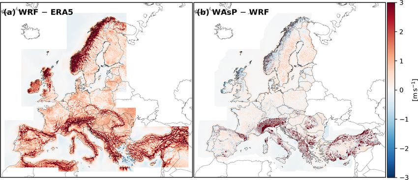
5080                                                                   M. Dörenkämper et al.: Making the NEWA – Part 2

   The initial evaluations of the wind conditions are typically   state-of-the-art models was needed (Petersen et al., 2013). To
based on numerical products, such as wind atlases, which          achieve this, the New European Wind Atlas (NEWA) project
generally provide convenient, fast, and easy access to esti-      was created as a 4-year research project with the goals of
mations of the characteristic wind conditions at a site. Wind     creating such a wind atlas, collecting relevant field measure-
atlases have a long history in wind energy siting applica-        ments for validation (Mann et al., 2017), and improving the
tions. In 1989, the European Wind Atlas (EWA, Troen and           model chain used for wind climate downscaling (Sanz Ro-
Petersen, 1989), one of the first comprehensive wind atlases,     drigo et al., 2020). The NEWA wind atlas (Petersen, 2017)
was published. It documents the meteorological basis for          (https://map.neweuropeanwindatlas.eu, last access: 20 Octo-
large parts of Europe and was the first wind atlas to be pro-     ber 2020). consists of mesoscale and microscale datasets that
duced using the wind atlas method, a collection of statisti-      cover all European Union member states, Norway, Switzer-
cal models that are the core of the Wind Atlas Analysis and       land, the Balkans, and Turkey. The mesoscale atlas was made
Application Program (WAsP) software package (Mortensen            using the Weather Research and Forecasting (WRF) model
et al., 2011). EWA was made based on a network of observa-        (Skamarock et al., 2008) and includes a number of both
tional masts covering much of Europe, whose measured wind         surface and boundary layer meteorological variables with a
climate served as the input to the WAsP model.                    3 km ×3 km grid spacing. The resulting data are available at
   Due to the ongoing advances of numerical weather pre-          seven wind energy relevant heights for 30 min intervals over
diction (NWP) models and the increase in available compu-         a 30-year period from 1989 to 2018. The WRF model output
tational resources, modern wind atlases are typically based       was downscaled using the WRF-WAsP methodology (Hah-
on numerical mesoscale model simulations. The wind cli-           mann et al., 2020) to create the microscale atlas, which is a
matologies (e.g. the long-term record of wind speed and di-       high-resolution atlas of the statistical wind climate covering
rection at various levels in the boundary layer) from these       the regions in a 50 m×50 m grid.
simulations, can be downscaled using a microscale model,             This paper is the second of two parts describing the mod-
which can be of different levels of complexity and accu-          elling involved in the making of the NEWA Wind Atlas: the
racy depending on the available computational resources and       first paper (Hahmann et al., 2020b) deals with the sensitiv-
the complexity of the area of interest. However, in regions       ity experiments that were carried out to guide the selection
with homogeneous surface conditions, such as over the sea,        of the WRF model configuration used for the production of
over large lakes, grasslands, or deserts, it may be adequate      the mesoscale model simulations of the wind atlas. This pa-
to use the output directly from a mesoscale model to create       per, the second part, focuses on the production of the wind
wind atlases, as in, e.g.Peña Diaz et al. (2011) and Doubrawa     atlas, including a selection of the results and the evaluation
et al. (2015). In regions with complex terrain, downscaling       of the wind atlas model chain using measurements from tall
using a microscale model is typically applied. For smaller        meteorological towers covering most of Europe.
regions like counties or federal states, statistical–dynamical       Throughout this paper, we describe the configuration and
downscaling based on meso-γ -scale or microscale Compu-           model adaptations that were used to create the products of
tational Fluid Dynamics (CFD) Reynolds-Averaged Navier–           the NEWA wind atlas. In addition, issues such as the com-
Stokes (RANS) models can be applied (as in, e.g. MWKEL,           putational challenges and resources needed for producing a
2013). For large regions, such as entire countries or conti-      mesoscale wind atlas for the European continent and the par-
nents, linearized flow models, such as WAsP, are most often       allelization of many millions of WAsP simulations are dis-
used to reduce the computational demands (see e.g. GWA,           cussed. Finally, we present an evaluation of the ability of the
2019; Mortensen et al., 2014).                                    final NEWA wind atlas to reproduce the spatial variability of
   Since the start of the century, wind atlases have been         the wind at a large number of tall masts in Europe. In Sect. 2
produced for a large number of countries, including Egypt         we introduce the models and the model setups and discuss
(Mortensen et al., 2006), South Africa (Mortensen et al.,         the computational aspects of the wind atlas generation. Sec-
2014; Hahmann et al., 2014, 2018), Finland (Tammelin et al.,      tion 3 presents the main results and the evaluation of the atlas
2013), Germany (Weiter et al., 2019), Greece (Kotroni et al.,     against mast data. In the last part of the paper, we discuss the
2014), Russia (Starkov and Landberg, 2000), and Iceland           results (Sect. 4), provide our conclusions (Sect. 5), and give
(Nawri et al., 2014), and for offshore regions, such as the       a short outlook for potential future work that may build upon
Great Lakes in the USA (Doubrawa et al., 2015), the off-          the results presented in this study.
shore Dutch Wind Atlas (Wijnant et al., 2019), the Southern
Baltic Sea (Peña Diaz et al., 2011), and the Southern North
Sea (Drüke et al., 2014). A comprehensive summary of na-
tional and regional wind atlases in Europe and can be found       2   Wind atlas generation
in Badger et al. (2018).
   With the ongoing technical, computational, and scientific      This section presents the mesoscale and microscale models
improvements since the release of EWA in 1989, a new up-          used in the NEWA model chain to create the wind atlas prod-
dated wind atlas for Europe using current best practices and      ucts. In addition to introducing the models and their setup,

Geosci. Model Dev., 13, 5079–5102, 2020                                           https://doi.org/10.5194/gmd-13-5079-2020
M. Dörenkämper et al.: Making the NEWA – Part 2 5081
the computational, technical, and logistical aspects of both
modelling activities are presented.
2.1 Mesoscale modelling: the WRF model
2.1.1 The WRF model
The mesoscale wind atlas was created using the WRF model
(Skamarock et al., 2008), which has a long record of use
for wind energy applications, both onshore and offshore (e.g.
Storm et al., 2009; Jimenez et al., 2010; Liu et al., 2011; Hor-
vath et al., 2012; Karagali et al., 2013; Hahmann et al., 2015;
Draxl et al., 2015; Dörenkämper et al., 2015; Lundquist et al.,
2019). The setup of the WRF model used for the NEWA wind
atlas is based on the evaluation of a large number of sensitiv-
ity experiments using mast data, which is documented in the
first part of this study (Hahmann et al., 2020b).
The mesoscale model simulations of the NEWA produc-
tion run use a modified version of the WRF model version
3.8.1, with changes in the Mellor-Yamada-Nakanishi-Niino
(MYNN) planetary boundary layer (PBL) scheme (for de-
tails see Sect. 5.2 in Hahmann et al., 2020b). Furthermore,
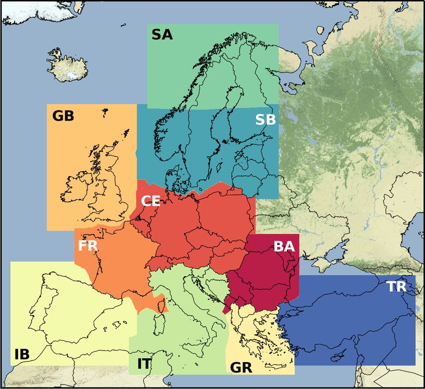
additional code that estimates ice accumulation was added to Figure 1. The location of 10 WRF model domains (D3) used in
the WRF model code. This icing model is based on the ice the NEWA production run, excluding a 30 grid point buffer around
each domain. The background map corresponds to D1, which is the
growth model from Makkonen (2000) and adds additional
same for all simulations. D2 domains are not shown Hasager et al.
output that can be used for estimating icing risk on wind tur- (reproduced from 2020).
bines.
The 30-year mesoscale database is created by running a
series of WRF model simulations: 7 d plus a 24 h spin-up most domain was run separately from the others. The 10 do-
period, which overlaps with the last day of the preceding mains were created using the following rules:.
weekly run. These relatively long simulations guarantee that
the mesoscale flow is in full equilibrium with the mesoscale 1. Domains have to cover the NEWA area of interest:
aerodynamic characteristics of the terrain, while nudging is all European Union member states, Norway, Switzer-
used to keep the model solution from drifting away from land, the Balkans, and Turkey, as well as offshore areas
the observed large-scale atmospheric patterns (Vincent and 100 km off each coast and the complete North and Baltic
Hahmann, 2015). An advantage of the weekly runs is that seas.
the simulations are independent of each other and can be in- 2. Domains should not include large regions outside the
tegrated in parallel. This reduces the total wall clock time NEWA area of interest.
needed to complete a multi-year climatology at a decent
computational overhead. However, the state of the lower 3. Domains must be large enough so that each country is
boundary, which is in equilibrium with the PBL conditions, fully covered in one domain (exceptions: Norway, Swe-
is lost after each re-initialization, necessitating the 24 h of den, and Finland).
spin-up time.
4. Domains must have sufficient overlap: at least 30 grid
All mesoscale simulations used three nested domains with
points buffer at each domain boundary (following Wang
a 3 km horizontal grid spacing for the innermost grid and
et al., 2019).
a 1 : 3 ratio between the inner and outer domain resolution,
leading to three different resolutions: 27 km for the outer do- The final domains vary in size from 325 × 343 grid points
main (D1) and 9 and 3 km for the inner nested domains D2 (GR) to 631 × 415 grid points (SB). All D2 domains have
and D3. The area to be covered by the NEWA wind atlas was a blending zone of 350 km (or 39 grid squares) around the
divided into 10 independent high-resolution computational respective D3 domain. The common outer D1 domain is
domains (named BA, CE, FR, GB, GR, IB, IT, SA, SB, and 250×220 grid points and corresponds to the background map
TR), as shown in Fig. 1. These are the innermost domains shown in Fig. 1.
(D3), which all share the common outermost domain (D1). All other final WRF model setup parameters of the NEWA
However, to further parallelize the simulations, each inner- production runs are summarized in Table 1. The above-
https://doi.org/10.5194/gmd-13-5079-2020 Geosci. Model Dev., 13, 5079–5102, 2020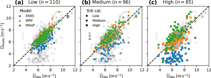
5082                                                                                            M. Dörenkämper et al.: Making the NEWA – Part 2

Table 1. Setup configuration used in the NEWA production run.

          WRF version                         3.8.1 (modified PBL + icing code)a
          Domains                             10 domains (see Fig. 1); Lambert conformal map projection
          Grid spacing (1x, 1y)               3 nests: 27 km (D1), 9 km (D2), 3 km (D3); one-way nesting
          Vertical discretization             61 vertical levels, model top at 50 hPa
          Model levels                        20 model levels below 1 km
                                              10 lowest level heights: approx. 6, 22, 40, 57, 73, 91, 113, 140, 171, 205 m a.g.l.
          Simulation length                   8 d including 24 h spin-up
          Terrain data                        Global Multi-resolution Terrain Elevation Data 2010 at 30 arcsec (Danielson and Gesch, 2011)
          Land use data                       CORINE 100 m (Copernicus Land Monitoring Service, 2019),
                                              ESA CCI (Poulter et al., 2015) where CORINE not available
          Dynamical forcing                   ERA5 (Hersbach and Dick, 2016) reanalysis (0.3◦ × 0.3◦ resolution) on pressure levels
          Sea conditions                      OSTIA (Donlon et al., 2012) SST and sea-ice (0.05◦ , approx. 5 km)
          Lake temperature                    Average ground temperature from ERA5,
                                              Lakes are converted to ocean when temperature is present in OSTIA
          Nudging                             Spectral nudging in D1 only, above PBL and level 20
          Time step                           Adaptive (< 5 % failed)
          PBL                                 MYNN (modified) (Mellor and Yamada, 1982)
          Surface layer                       MO (Eta similarity) (Janjic and Zavisa, 1994)
          Land surface model                  NOAH-LSM (Tewari et al., 2004)
          Cloud microphysics                  WRF single-moment five-class scheme (Hong et al., 2004)
          Radiation                           RRTMG scheme, 12 min calling frequency (Iacono et al., 2008)
          Cumulus parameterization            Kain–Fritsch scheme on D1 and D2 (Kain, 2004)
          Icing                               WSM5 (Hong et al., 2004) + icing code + sum of qcloud and qice
          Diffusion                           Simple diffusion
                                              2D deformation
                                              6th-order positive definite numerical diffusion
                                              Rates of 0.06, 0.08, and 0.1 for D1, D2, and D3
                                              Vertical damping
          Advection                           Positive definite advection of moisture and scalars
          Numerical options                   480 cores, IO quilting (one node used for output)
        a The WRF code modifications are available from the NEWA GitHub repository: https://github.com/newa-wind/Mesoscale (last access: 20 October 2020).

mentioned WRF model code modifications, as well as the                                  100 TB of project space (for storing, e.g. reanalysis input data
namelists and domain files for all 10 domains, are avail-                               and scripts) was available on the system.
able from the NEWA GitHub repository (https://github.com/                                  As described in Sect. 2.1.1, the final setup for the pro-
newa-wind/Mesoscale, last access: 20 October 2020).                                     duction run was divided into 10 domains covering the EU,
                                                                                        plus Norway, Switzerland, and Turkey. The estimated total
                                                                                        mesoscale model output raw data (10 domains over 30 years)
2.1.2     Computational aspects                                                         in 3 km spatial and 30 min temporal resolution would have
                                                                                        resulted in a total of 6 petabytes. However, the final post-
                                                                                        processed wind atlas resulted in a much lower volume of
The production run for the NEWA mesoscale was conducted
                                                                                        around 0.2 petabytes (see below). Consequently, a partition-
between August 2018 and March 2019 on the MareNos-
                                                                                        ing of the full run into smaller runs that fit into the 100 TB of
trum 4 supercomputer that is operated by the Barcelona
                                                                                        scratch space was essential, as was a high degree of automa-
Supercomputing Center (BSC). For this purpose, compu-
                                                                                        tion of the runs, the post-processing, and the data transfer.
tational resources to the amount of 57 million core hours
                                                                                           Figure 2 illustrates the split of the full wind atlas into sep-
were granted to the consortium via a PRACE (Partnership
                                                                                        arate computational tasks and the degree of automation of
for Advanced Computing in Europe) proposal. The PRACE
                                                                                        each part of the job chain. The full 30-year wind atlas for
project was active, and the resources were available between
                                                                                        all 10 domains was first subdivided by the year and then by
April 2018 and March 2019. Besides the computational re-
                                                                                        the domain. Each year–domain run (300 runs in total) then
sources in terms of core hours, 100 terabytes (TB) of scratch
                                                                                        contained three array jobs of 52 or 53 elements each, one
space (for the temporary files of the runs) and an additional

Geosci. Model Dev., 13, 5079–5102, 2020                                                                       https://doi.org/10.5194/gmd-13-5079-2020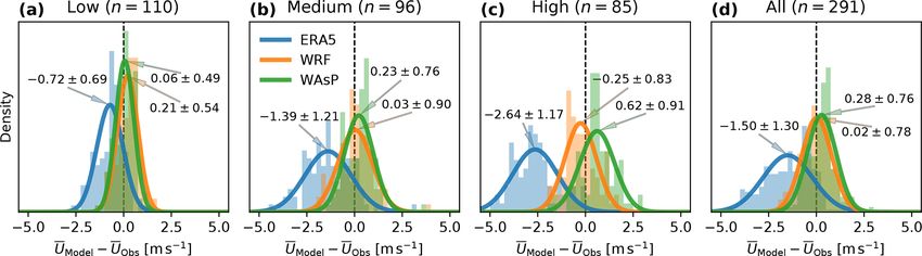
M. Dörenkämper et al.: Making the NEWA – Part 2                                                                                5083

                                                                        In total, each year–domain run occupied about 20 TB
                                                                     (from 13 TB for the GR domain to 23 TB for the SB do-
                                                                     main) of scratch space, including all raw and post-processed
                                                                     data. Thus, it was possible to have up to five year–domain
                                                                     sets running at the same time within the space provided on
                                                                     MareNostrum 4. After a year–domain set completed success-
                                                                     fully (i.e. the post-processing array run completed), a script
                                                                     for file checks, transfer, and cleanup was started. The file-
                                                                     check portion of the script checked the post-processed output
                                                                     files for consistency and completeness. If the check proved
                                                                     successful, the post-processed files were moved to a special
                                                                     transfer directory and the raw data were deleted. On a dedi-
                                                                     cated server at the Technical University of Denmark (DTU),
                                                                     a cron job was constantly watching for post-processed files in
                                                                     the aforementioned transfer directory and initiated the trans-
                                                                     fer to the DTU server when new post-processed files were
                                                                     found.
                                                                        During the production run, between August 2018 and
                                                                     March 2019, the mesoscale working group of the NEWA
                                                                     consortium (the authors of this study and further supporters)
                                                                     was constantly on standby. Each week a different person was
                                                                     on duty to launch, check, resubmit, and transfer runs 7 d a
                                                                     week to ensure fast progress and to avoid longer idle periods.
                                                                        In terms of computational costs, each year–domain config-
                                                                     uration spent 80 000–140 000 core hours, leading to a total
                                                                     of about 35 million core hours for the full wind atlas. (The
                                                                     remaining PRACE grant was used for ensemble run calcu-
                                                                     lations; see, e.g. González-Rouco et al., 2019). The resulting
                                                                     post-processed mesoscale time series (daily netCDF files fol-
                                                                     lowing CF-1.6 conventions) contained the parameters given
                                                                     in Appendix A. The mesoscale wind atlas (30 years, 10 do-
Figure 2. Illustration of how the production run was conducted.      mains, 30 min resolution, 7 vertical levels) resulted in a total
The dashed line encloses fully automatic processes, the dark grey    volume of around 160 TB.
box encloses the parallel process (here 480 cores), and light grey      The final NEWA mesoscale wind atlas was created by
boxes enclose serial processes.
                                                                     combining the results from the individual mesoscale domains
                                                                     into a single merged mesoscale dataset for public use. Fig-
for each of the weekly runs. Out of these three array jobs,          ure 3 shows how each domain contributed to the combined
only the execution of the mesoscale run itself (real.exe             domain. Because all domains shared the same outer domain,
and wrf.exe from WRFV3.8.1, indicated by the dark grey               reference location, and projection, the grid nodes of neigh-
colour in Fig. 2) were run in parallel, using 480 cores each.        bouring domains overlap exactly, and therefore no interpola-
All other tasks were run serially (light grey colour in Fig. 2).     tion was needed to combine them. Whenever possible, data
   The setup and submission of each year–domain set (three           for each country’s exclusive economic zone come from the
array jobs of 52 or 53 weeks each) was automated using a             same mesoscale domain (cf. Fig. 1).
python3 script adapted to the properties of the computing
cluster. It linked, copied, and adapted the necessary input          2.2     Microscale modelling
files (e.g. namelists) and then submitted the job scripts to the
queuing system. Dependencies were setup between each of              2.2.1    The WRF-WAsP methodology
the three stages of the job arrays to allow a full automation of
the simulation process. This means that the array of jobs re-
sponsible for post-processing automatically started after the        The horizontal grid spacing of the mesoscale atlas is 3 km
main runs were completed. In case of problems (e.g. hard-            (in each direction) and cannot capture local flow features
ware issues), a different script was used to manually resubmit       from sub-grid variations in orography and surface roughness.
single weeks of a year–domain run.                                   However, capturing these effects can be vital for accurately
                                                                     determining the local wind climate at a site (Sanz Rodrigo
                                                                     et al., 2017).

https://doi.org/10.5194/gmd-13-5079-2020                                               Geosci. Model Dev., 13, 5079–5102, 2020
5084                                                                     M. Dörenkämper et al.: Making the NEWA – Part 2

                                                                    the same maps, the elevation and land use from the WRF
                                                                    model is used for “removing” topographical effects, and the
                                                                    best available maps are used for “adding” topographical ef-
                                                                    fects. In WAsP, the wind climate at a given location is defined
                                                                    as the probability density of wind speed and wind directions.
                                                                    It can be represented as the probability density binned into a
                                                                    number of equal-width wind speed and wind direction bins
                                                                    or as a set of frequencies and best-fit Weibull distribution pa-
                                                                    rameters for each sector.
                                                                       As outlined above, the typical WRF-WAsP procedure in-
                                                                    volves two steps. First, the WRF model wind climate is “gen-
                                                                    eralized”, which removes the WRF local terrain effects from
                                                                    the WRF-simulated wind climate (i.e. the wind speed and
                                                                    sector statistics) to produce a new wind climate that is rep-
                                                                    resentative of a larger area surrounding the model grid cell.
                                                                    The generalized wind climate (in WAsP terminology) corre-
                                                                    sponds to the wind field distribution that would exist without
                                                                    orography and a homogeneous surface roughness, i.e. a flat
                                                                    surface of constant surface roughness. Therefore, the gen-
                                                                    eralized wind climate varies only with height. In the WRF-
Figure 3. Map showing how the individual mesoscale domains are
combined into a single merged dataset. Whenever possible the data   WAsP process, each generalized wind climate holds informa-
for each country’s exclusive economic zone come from the same       tion, not just of the wind field distribution for a single surface
domain. The background is the stamen terrain background from        roughness and height above ground level (a.g.l.) but instead
http://maps.stamen.com/terrain-background (last access: 30 Octo-    for a number of preselected surface roughnesses and heights.
ber 2020) – © OpenStreetMap contributors 2020. Distributed under    In the second step, local terrain effects are “applied” to the
a Creative Commons BY-SA License.                                   generalized wind climate, resulting in a predicted wind cli-
                                                                    mate. The local terrain effects vary based on the site location
                                                                    and height above the surface. The generalization procedure is
   Downscaling of the WRF-derived climatologies with a              carried out for all WRF model grid points, and the prediction
microscale model is needed for more accurate wind data,             procedure is carried out at each microscale model grid point
especially in non-homogeneous terrain. For this purpose,            and desired height. This results in a high-resolution map of
the WAsP microscale model was used (Troen and Petersen,             the wind climate, i.e. the microscale wind atlas. The mean
1989), following the WRF-WAsP downscaling methodology               wind speed at 100 m for the microscale wind atlas is pre-
(Hahmann et al., 2014; Badger et al., 2014). Linearized flow        sented in Fig. 6c. The default procedure of WAsP is to repre-
models, such as the WAsP model, are well known and have             sent the wind climate as binned wind speeds and directions
been extensively used within the wind energy sector for site        during the generalization step until all corrections have been
assessment in the past 30 years. Because the WAsP flow              applied, then Weibull fits are made and used in subsequent
model is simple and computationally efficient, it can be ap-        steps.
plied to large areas.                                                  In the WRF-WAsP methodology, the terrain effects for the
   The underlying principle of the WAsP methodology is to           generalization are derived from the gridded WRF model el-
estimate the wind climate at a point by extrapolating hori-         evation and surface roughness, while the terrain effects used
zontally and vertically from a measured wind climate at a           for prediction are estimated using the best available high-
nearby point. The extrapolation is done by first “removing”         resolution maps of elevation and surface roughness. The de-
topographic effects (orographic, roughness, and obstacles)          tailed technique for how these effects are calculated and used
from the known wind climate estimated by the linearized             is described in Badger et al. (2014) for the mesoscale gener-
flow model from the topographical maps of the area sur-             alization and Troen and Petersen (1989) for the microscale
rounding the known site. Then, vertical extrapolation is done       prediction. All effects are taken into account using the de-
using drag law relations. Finally, the topographic effects (es-     fault treatment of atmospheric stability in WAsP, which over
timated by the same model) at the target point are added to         land corresponds to an average heat flux of −40 W m−2 and
the wind climate. This method only works for short distances        root mean square of 100 W m−2 and over sea corresponds
where it can be assumed that the geostrophic forcing remains        to an average heat flux of 15 W m−2 and root mean square
constant.                                                           of 30 W m−2 .
   The WRF-WAsP downscaling used here is analogous to                  The NEWA long-term wind atlas, based on the 30 years of
the one used with a measured wind climate. However, instead         WRF model data, was made using the default WRF-WAsP
of removing and adding topographical effects estimated from         downscaling method described above. The WRF model wind

Geosci. Model Dev., 13, 5079–5102, 2020                                              https://doi.org/10.5194/gmd-13-5079-2020
M. Dörenkämper et al.: Making the NEWA – Part 2                                                                             5085

climates from these 30 years were generalized to heights of        However, in the WRF vegetation table, they are both assigned
50, 75, 100, 150, and 200 m a.g.l. and to surface roughnesses      a value of 0.10 m, which – everything else being equal – re-
of 0.0002, 0.03, 0.1, 0.4, and 1.5 m. Subsequently, predic-        sults in a large increase in the predicted wind speed when
tions were made at heights of 50, 100, and 200 m a.g.l. on a       downscaling the WRF data for these classes. Similarly, lo-
50 m × 50 m horizontal grid across Europe.                         cations with high z0 values, such as forests and urban areas,
                                                                   experience the opposite effect. Therefore, the adjustment to-
2.2.2   High-resolution surface datasets                           wards the WRF roughness values can be viewed as making
                                                                   the WAsP roughness corrections more conservative. For both
The high-resolution terrain elevation was created by com-          the WRF simulations and the WAsP downscaling, the surface
bining the Shuttle Radar Topography Coverage Version 3             roughness values do not change with the seasons and are as-
(SRTM v3) dataset (Farr et al., 2007) south of 60◦ N and           sumed to represent a seasonal geometric average.
the ViewFinder DEM (de Ferranti, 2014) north of 60◦ N.
Both of these datasets have a 3 arcsec (≈ 90 m) resolution         2.2.3   Computational aspects
and are provided in the WGS84 map projection. The high-
resolution surface roughness length (z0 ) values were created      For easy interfacing with the WAsP model, the “PyWAsP”
based on the 2018 CORINE land cover dataset (Copernicus            (PyWAsP, 2020) software package developed at DTU was
Land Monitoring Service, 2019), which has a horizontal res-        used. PyWAsP is a python wrapper around the (mostly)
olution of 100 m and is in the ETRS89 Lambert Azimuthal            Fortran-based WAsP core. The WAsP calculations are inde-
Equal-Area map projection (EPSG 3035).                             pendent, making the downscaling procedure an “embarrass-
   For downscaling with WAsP, the CORINE land cover                ingly parallel” problem. However, to facilitate the 5.6 billion
classes were related to constant z0 values through a lookup        WAsP calculations that needed to be done, a two-tier par-
table (Table 2, “WAsP” column). Since no objective or thor-        allelization process was employed, taking advantage of the
oughly validated land use to surface roughness conversion          cluster architecture used.
exists for the CORINE land use classes, the accuracy of the           First, to split the work into manageable chunks, the wind
table is highly uncertain. For WRF, the 44 CORINE land use         atlas area was divided into 1402 tiles, each covering an
classes were converted to the most similar 21 class USGS           area of 100 km×100 km, and thereby consisting of 2000 ×
(Anderson et al., 1976) and converted to surface roughness         2000 calculation points (the target locations) spaced 50 m
length using constant values first suggested by Pineda et al.      apart, adding up to the 5.6 billion calculations mentioned
(2002) (see Table B1 in Appendix B for further details).           above. The tiles and all WAsP modelling was defined in
Silva et al. (2007) proposed surface roughness values for the      the ETRS89 Lambert Azimuthal Equal-Area map projection
CORINE land use classes, but these were only validated for         (EPSG 3035) in metric units of metres. Each tile was submit-
three sites in Portugal. A different conversion table, referred    ted to a single computational node, with the load balancing of
to as the DTU table, was proposed (Rogier R. Floors, Niels         tile jobs managed by the HPC workload manager. To take ad-
G. Mortensen, Andrea N. Hahmann, personal communica-               vantage of the 32 CPU cores on each compute node, each tile
tion, DTU Wind Energy, March 2019) but has likewise not            was divided into 2500 sub-tiles of 40 × 40 calculation points.
been comprehensively validated.                                    The dask python package was used for scheduling and dis-
   The z0 values in the “WAsP” column in Table 2 were de-          tribution of the computations needed for each of the sub-tiles
termined by using the DTU table as a starting point and then       across the different CPU cores.
adjusting the values toward the corresponding z0 in the WRF           To allow for each tile to operate as a stand-alone compu-
model table (Table 2, “WRF” column). Since the values in           tational task, terrain and generalized wind climate data were
the DTU table are defined for the 44 CORINE classes, each          created for each tile in advance. Natural neighbour interpo-
class has a better characterization of a specific land use type.   lation (Sibson, 1981) was used to interpolate the generalized
In contrast, each of the 21 USGS classes needs to represent        wind climates computed from the mesoscale model output
a broader range of land use types. This means that the DTU         to each target location. To ensure that a sufficient number of
table has more variation than the USGS table, and in most          input wind climates were available around each target loca-
cases low roughness land use types have much lower z0 val-         tion for the interpolation, the wind climates included a 10 km
ues and high roughness land use types have much higher             buffer region around each tile.
ones. The WAsP z0 values were adjusted to be more like the            Following WAsP best practices (Mortensen, 2018), a
WRF values to reduce the difference in the effective surface       buffer area of 25 km around the tile should be enough to ac-
roughness between the two models and therefore reduce the          curately model the influence of the orographic and surface
risk of overcorrecting the wind climate when using the mi-         roughness maps. However, this assumes some human judge-
croscale model. For example, “non-irrigated arable land” and       ment in the creation of the surface roughness map. WAsP
“pastures” are common land use classes in Europe (Table 2,         uses the z0 map in a couple of different ways. First a rough-
“Proportion” column), and are respectively assigned rough-         ness rose is created. It contains information about upstream
nesses of 0.05 and 0.03 m in the DTU table (not shown).            roughness changes in a number of radial sectors (typically

https://doi.org/10.5194/gmd-13-5079-2020                                             Geosci. Model Dev., 13, 5079–5102, 2020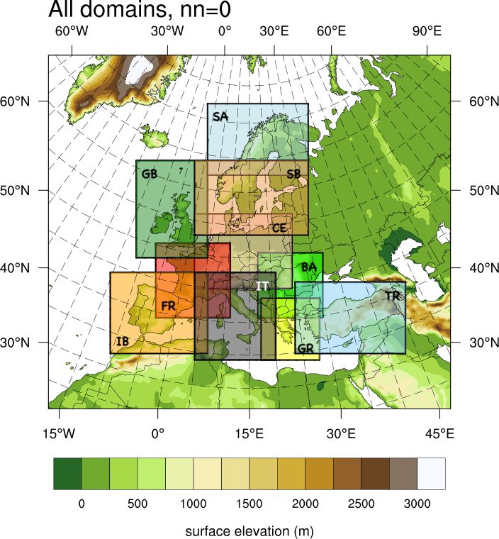
5086                                                                                M. Dörenkämper et al.: Making the NEWA – Part 2

Table 2. Surface roughness length [m] for each land use category in WAsP and WRF and the proportion it represents in the total dataset.

  Category                                   Proportion   WAsP      WRF        Category                      Proportion   WAsP       WRF
                                                   (%)    z0 (m)   z0 (m)                                          (%)    z0 (m)    z0 (m)
  Continuous urban fabric                          0.1      1.0       1.0      Broad-leaved forest                 8.0        1.0       0.9
  Discontinuous urban fabric                       2.3      1.0       1.0      Coniferous forest                  11.1        1.2       0.9
  Industrial or commercial units                   0.4      0.7       0.5      Mixed forest                        4.2        1.1       0.5
  Road and rail networks and assoc. land           0.1      0.2       0.5      Natural grasslands                  2.9        0.1       0.1
  Port areas                                     < 0.1      0.5       0.5      Moors and heathland                 2.4       0.12     0.12
  Airports                                       < 0.1      0.1       0.5      Sclerophyllous vegetation           1.5       0.12     0.12
  Mineral extraction sites                         0.1     0.15       0.5      Transitional woodland-shrub         4.1        0.4     0.12
  Dump sites                                     < 0.1     0.15       0.5      Beaches – dunes – sands             0.1       0.01     0.01
  Construction sites                             < 0.1      0.3       0.5      Bare rocks                          1.3      0.05      0.01
  Green urban areas                              < 0.1      0.8       0.5      Sparsely vegetated areas            3.2       0.03     0.01
  Sport and leisure facilities                     0.2      0.3       0.5      Burnt areas                       < 0.1        0.2      0.01
  Non-irrigated arable land                       16.5      0.1       0.1      Glaciers and perpetual snow         0.2     0.005     0.001
  Permanently irrigated land                       1.5      0.1       0.1      Inland marshes                      0.2      0.05     0.001
  Rice fields                                      0.1      0.1       0.1      Peat bogs                           1.6       0.03    0.001
  Vineyards                                        0.6      0.3       0.2      Salt marshes                        0.1      0.02     0.001
  Fruit trees and berry plantations                0.6      0.4       0.2      Salines                           < 0.1     0.005     0.001
  Olive groves                                     0.7      0.4       0.2      Intertidal flats                    0.2     0.001     0.001
  Pastures                                         5.7      0.1       0.1      Water courses                       0.2    0.0002    0.0001
  Annual crops assoc. with perm. crops             0.1      0.2       0.2      Water bodies                        1.8    0.0002    0.0001
  Complex cultivation patterns                     3.3      0.2       0.2      Coastal lagoons                     0.1    0.0002    0.0001
  Agriculture with sig. areas of nat. veg.         3.7      0.2       0.2      Estuaries                           0.1    0.0002    0.0001
  Agro-forestry areas                              0.5      0.5       0.2      Sea and ocean                      20.1    0.0002    0.0001

12) and its distances to the point. For computational effi-                 rose, and (4) calculate the roughness site effects using the
ciency only the roughness changes that most impact the flow                 updated roughness rose. The computational time for the sim-
is kept (10 at most). These are identified based on the amount              ulation of the tiles varied considerably, between 1 and 14 h
of total roughness variation they account for. The roughness                for each tile, depending on the complexity of the terrain.
rose is then used to calculate the upstream “background”
roughness for the point and to model the internal bound-                    2.3     Evaluation methodology
ary layers caused by the roughness changes. One of the key
limitations of this approach is that the model assumes that                 It is not possible or appropriate to evaluate the wind climatol-
the last roughness in the roughness rose continues to be the                ogy of the wind atlas itself (e.g. what is available for down-
roughness indefinitely. Therefore, when creating a roughness                load from the NEWA site) because it represents a long cli-
map, it is important to look further upstream when making                   matological period (1989–2018) and no wind speed measure-
the map and to ensure that the outer roughness values match                 ments span that entire period at wind energy relevant heights.
those found further upstream of the site. However, in our au-               Instead, the NEWA model chain is validated by using it to
tomated process this is not possible. This led to sensitivities             create individual wind climates for 291 tall masts covering
in the sub-tile results, due to the inclusion of additional up-             Europe, such that the wind climates represent the exact mea-
stream roughness values when calculating the background                     surement periods covered by each mast. This section covers
roughness. To limit this impact, we included a preprocess-                  the metrics used to describe the terrain complexity at each
ing step that calculated the background roughness at a 1 km                 site, followed by a description of the masts’ measurement
grid spacing using roughness maps that extended 100 km up-                  data. Finally, we describe a number of modifications to the
stream from the grid point. When calculating the predicted                  WRF-WAsP methodology made specifically for the evalua-
wind climate, a 25 km map was used, but the preprocessed                    tion against mast data.
background roughness from a point approximately 30 km up-
stream was inserted into the roughness rose as the last rough-              2.3.1    Terrain complexity
ness to reduce the sub-tile sensitivity.
   In summary, to provide the correct background roughness                  To quantify the relationship between model biases and the
to the WAsP model, the following steps were carried out for                 complexity of the terrain at the sites, several metrics related
each sub-tile: (1) get coarse background roughness from a                   to the orographic and surface roughness complexity were cal-
pre-processed map, (2) create the roughness rose, (3) add                   culated for each site. In this paper we focus on the rugged-
coarse background roughness as the last bin of the roughness                ness index (RIX) (Mortensen et al., 2008), which was used to

Geosci. Model Dev., 13, 5079–5102, 2020                                                      https://doi.org/10.5194/gmd-13-5079-2020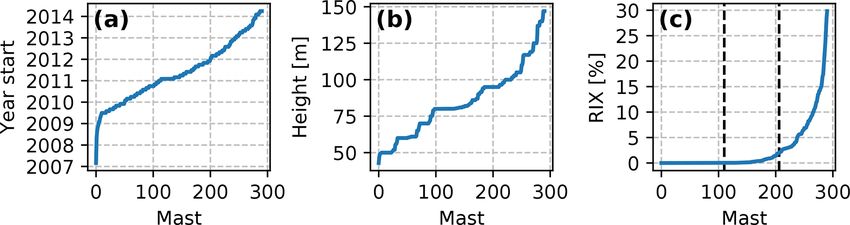
M. Dörenkämper et al.: Making the NEWA – Part 2                                                                                   5087

quantify the orographic complexity. The RIX number is de-
fined as the fractional extent of the terrain that exceeds a crit-
ical slope, in this case 16.7 ◦ , within 3500 m of the point of
interest. The RIX number is used in WAsP to indicate terrain
where the surrounding orographic slopes are steeper than the
valid limits of the flow model (IBZ Jackson and Hunt, 1975)
and thus where the orographic speed-ups are expected to be
overestimated.
   Additionally, three metrics to quantify the surface rough-
ness heterogeneity were investigated for each site. First, the
degree of variation of the surface roughness around the sites
was used to identify sites that would likely have complex
structures in the flow due to rapid changes in the surround-
ing surface roughness. Second, the distance from the mast
location to the nearest coastline was used to detect coastal
influences on the model biases. Third, the average aggregate
upstream surface roughness at the site was used to detect bi-
ases associated with high or low roughness sites.
   Initial analysis showed that each of the surface roughness
metrics explained some of the variance of the model biases.          Figure 4. The number of masts located in each country in Europe.
However, it was clear that the RIX number explained most of          For several smaller countries the number has been omitted for read-
the variance for both the ERA5 and WAsP results and a large          ability (all of them have zero masts).
amount of the variance in the WRF model results. Therefore,
only the RIX number is included in the remaining analysis.
                                                                     (e.g. repeated) signals for this study based on 10 min av-
2.3.2   Observed data                                                erages; fortunately no problems were detected. Because no
                                                                     flow distortion correction was made to measurements from
The results of the NEWA model chain were validated against           masts with a single instrument at the measurement height, we
measurements from 291 tall masts made available for the              expect flow distortion to have some influence on the results.
study. Because the data are proprietary, only aggregated re-         We estimate the effect to be up to a few percent difference in
sults are presented. Figure 4 shows the number of masts              annual mean wind speed for those masts, based on the impact
located in each country. Large variations in the number of           of including such correction in Hahmann et al. (2020b) and
masts present in each country and across regions exist, e.g.         indications by, for example, Westerhellweg et al. (2012).
just 4 masts in Germany and Spain, while 38, 42, and 44                 A total of 12 months of measurements were used from
masts are located in Poland, Italy, and Turkey, respectively.        each mast to ensure that the results were not biased due
However, most parts of Europe and Turkey are well repre-             to differences in sample sizes. The period with the highest
sented.                                                              availability of measurements (between 2007 and 2015) was
   Figure 5 shows the distribution of several descriptive vari-      chosen. For most masts, the best period occurred after 2009
ables for the 291 masts. All measurements used in the eval-          (Fig. 5a). To avoid biases due to seasonal variations in data
uation were taken on tall meteorological masts. Cup or sonic         availability, an additional requirement that at least 80 % of
anemometers were used for the wind speed measurements,               the possible data were available for each month was stipu-
either from a single instrument or via an optimal sampling           lated. For most masts, more than 90 % of the possible data
of measurements from two instruments mounted on oppos-               were recovered every month.
ing booms to reduce flow distortion effects. Only measure-              The RIX values for the masts (Fig. 5c) shows a skewed
ments 40–150 m a.g.l. were used for the evaluation (Fig. 5b)         distribution, with most values found below 2 %, and only a
in order to avoid the large uncertainties associated with wind       few masts with very large values. For further analysis, the
speed measurements near the surface and to ensure that the           masts were grouped into three RIX groups: low: 0 % (n =
measurements are representative of modern and future tur-            110); medium: 0 %–2 % (n = 96); and high: 2 % (n = 85) or
bine hub heights. Wind direction measurements were taken             greater (dashed lines in the figure). These thresholds were
either from the sonic anemometers or from wind vanes as              chosen to ensure a similar number of masts in each group.
close to the wind speed measurements as possible (typically
0–40 m below the wind speed instrument). The measure-
ments were previously quality controlled by applying an in-
house method of the data provider and were further checked
for obvious measurement errors like icing and non-physical

https://doi.org/10.5194/gmd-13-5079-2020                                                Geosci. Model Dev., 13, 5079–5102, 2020
5088 M. Dörenkämper et al.: Making the NEWA – Part 2
Figure 5. Ranked values of metadata variables for the 291 masts: (a) the start year of the 1-year period, (b) the height a.g.l. of the wind speed
measurements, and (c) the ruggedness index (RIX). The dashed vertical lines in (c) shows the separation (greater than 0 % and greater than
2 %) of the masts into groups by RIX.
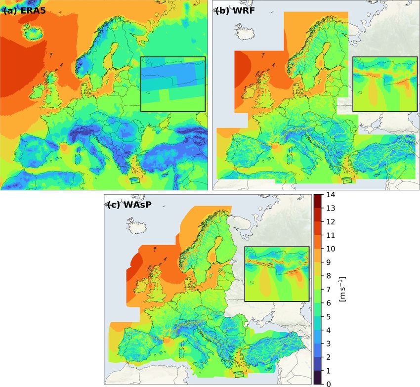
Figure 6. (a) ERA5, (b) WRF, and (c) WAsP mean wind speed at 100 m a.g.l. averaged over the full 30-year period (1989–2018). The zoom-in
shows the results for the island of Crete. Additional details can be seen on the NEWA wind atlas website https://map.neweuropeanwindatlas.
eu/ (last access: 20 October 2020). The map background is the stamen terrain-background from http://maps.stamen.com/terrain-background
(last access: 20 October 2020) – © OpenStreetMap contributors 2020. Distributed under a Creative Commons BY-SA License.
2.3.3 Adjustments to WRF-WAsP downscaling used and prediction) with Weibull-fitting used after the general-
for evaluation against mast data ization step, the corrections due to terrain effects from both
steps were applied to the binned wind climate during the
same (single) step. Third, since the WRF output was inter-
For evaluation of the downscaled wind climate at each mast polated to 50, 75, 100, 150, and 200 m, we used the height
site, some modifications to the WRF-WAsP methodology closest to the height of the measurements, thus the largest
were made. First, the measurements and the WRF model data vertical extrapolation required was less than 25 m and on av-
for the mast location (nearest grid cell) were obtained, en- erage it was just 6.8 m. The probability density of the orig-
suring that the WRF data were concurrent to the measure- inal bin is distributed to the nearest bins in the new binned
ments. Second, instead of a two-step process (generalization
Geosci. Model Dev., 13, 5079–5102, 2020 https://doi.org/10.5194/gmd-13-5079-2020M. Dörenkämper et al.: Making the NEWA – Part 2 5089
wind climate. After repeating this for every bin of the orig- Additional terrain effects along large mountain ridges can
inal wind climate, the new predicted binned wind climate is be seen, including the highest wind speeds in Europe, occur-
complete. Neutral atmospheric stability was assumed for the ring in Central Norway, and areas in the Alps that have wind
vertical extrapolation from WRF output height to the height speeds above 10 m s−1 . As expected, the microscale down-
of the measurements, and the stability correction of Weibull scaling results in larger flow variations in mountainous areas,
parameters (Troen and Petersen, 1989), which is normally as exemplified in the inset figure. Thus, the wind speeds on
made to the generalized wind climate, was omitted. the mountain tops are slightly higher.
This alternative approach has some advantages over the Figure 7 shows the differences in the 100 m mean wind
default approach: a Weibull distributed wind is not assumed, speed between WRF and ERA5 (a) and WAsP and WRF
so no parameterization biases occur. This is a particular ad- (b) for the full 30-year period. To calculate the differences
vantage for shorter periods, i.e. months, but may also be ad- the lower-resolution data were interpolated bi-linearly to the
vantageous for 1-year periods, such as those used here. Also, grid of the higher-resolution dataset, which is not typically
when the generalization and prediction is done in one sin- recommended, but is done here for illustration purposes. For
gle step, one avoids the truncation errors that occur when the convenience, the difference between WAsP and WRF was
wind climate is generalized to fixed generalization heights not calculated on the native 50 m WAsP grid but on a down-
and surface roughness and then subsequently interpolated to sampled grid corresponding to every 10th point in north and
a new height and surface roughness for the predicted wind east directions, i.e. with a 500 m×500 m spacing. In general,
climate at the site. The impact of these differences between it is clearly visible that the mesoscale model resolves the ter-
the default WRF-WAsP approach and the alternative ap- rain better than the reanalysis and thus captures more of the
proach was estimated for the 1-year wind climates at the val- variation due to orography, e.g. the larger wind speed on top
idation sites. For the mean wind speed, the differences are of of mountain ridges. On the large European scale, however,
the order of one percent due to Weibull-fitting and similarly the differences between mesoscale and microscale are small,
for the stability correction. A direct comparison between the especially in areas of low terrain complexity. However, over
WRF-WAsP downscaling over the entire map and that at the very complex topography (e.g. in the Alps and Pyrenees) the
sites is not possible, but the differences should similarly be WAsP downscaling greatly increases the wind speed. This is
on the order of a few percent. This issue is discussed further studied in more detail in Sect. 3.2.
in Sect. 4. The post-processed mesoscale and microscale fields can
be accessed interactively on the NEWA website: https://map.
neweuropeanwindatlas.eu/ (last access: 20 October 2020).
3 Results
3.2 NEWA model chain evaluation
3.1 The wind atlas
Figure 6 shows one of the main results of the NEWA wind The evaluation of the NEWA model chain performed
atlas, the map of the wind speed at 100 m averaged over the by comparing the wind climates estimated at each
full 30-year period (1989–2018) derived from the mesoscale stage of the model chain: ERA5 (forcing reanalysis),
simulations and downscaling with WAsP. The difference in ERA5+WRF (mesoscale, simply labelled “WRF”), and
the wind speed between onshore and offshore sites is evident ERA5+WRF+WAsP (microscale, simply labelled “WAsP”)
in many areas. Local wind systems like the Mistral, the Bora, to the observed wind climates. By comparing the wind cli-
and the flow through the Strait of Gibraltar (Levante and mates, it is not possible to evaluate the time-dependent as-
Poniente) are clearly visible. Due to the limited resolution, pects of the NEWA model results, which, additionally, are
some of these flows are not fully resolved in commonly used not available from the WAsP model. Further analysis of time-
reanalysis datasets like ERA5 (Hersbach and Dick, 2016) dependent aspects are included in the NEWA uncertainty re-
and CFSRv2 (Saha et al., 2014) or MERRA2 (Gelaro et al., port (González-Rouco et al., 2019).
2017) (not shown here). The inset figures in Fig. 6 show the The WRF- and ERA5-derived wind climates are calcu-
flow around the Greek island Crete, which is heavily influ- lated from the time series of wind speed and direction, and
enced by the Etesian winds. ERA5 and WRF both capture interpolated linearly in time and space to the mast location
these winds, but differ significantly in magnitude over and in and height for times concurrent with the measurements. The
the lee of Crete. It is also clear that additional flow features WAsP wind climates were estimated using the method out-
have been resolved by WRF, e.g. gap flows in the mountains lined in Sect. 2.2.
of Crete. The microscale downscaling with WAsP adds ad-
ditional details especially over the complex coastal moun- 3.2.1 Mean wind speed biases
tain ridges. Additional details and a comparison with satellite
data for this local wind system are provided in Hasager et al. The relationship between the observed and modelled mean
(2020). wind speeds for the validation periods for the 291 masts are
presented in Fig. 8. The same point scatter is repeated in
https://doi.org/10.5194/gmd-13-5079-2020 Geosci. Model Dev., 13, 5079–5102, 20205090 M. Dörenkämper et al.: Making the NEWA – Part 2 Figure 7. Mean wind speed differences for WRF minus ERA5 (a) and WAsP minus WRF (b) at 100 m a.g.l. averaged over the full 30-year period (1989–2018). Note that the lower resolution data were interpolated bi-linearly to the grid of the dataset with higher resolution. The difference between WAsP- and WRF-derived winds was calculated on a down-sampled version of the WAsP grid with a grid spacing of 500 m×500 m. Figure 8. Observed versus modelled mean wind speed for ERA5, WRF, and WAsP. The three subplots include the same scatter points, but each of them highlight a different ruggedness index (RIX) category: low (a), medium (b), and high (c). The number of masts (n) in each category is indicated above the subplots. three subplots, each with samples from one of the three RIX both ERA5 and WRF, the spread for biases in the mean wind groups highlighted with colours and the remaining samples speed are comparable between the samples in medium and greyed out (Fig. 8). The corresponding distributions of mean high RIX classes, but slightly smaller for high RIX. wind speed biases, computed as the model minus the obser- The mean biases in wind speed from WAsP and WRF are vation values, are shown in Fig. 9. The smallest spread and most similar in simple terrain, where the WAsP model makes least scatter in mean wind speed from all three downscaling the smallest adjustments to the WRF model wind climates stages (ERA5, WRF and WAsP) is at low RIX sites and is (Fig. 9). The adjustments that are made by WAsP cause a considerably larger at medium and high RIX sites. This re- reduction in the bias relative to the ones from WRF (from sult is not unexpected and shows that the uncertainty in all 0.21 to 0.06 m s−1 ) and spread (from 0.54 to 0.49 m s−1 ). The three models increases as the orographic complexity of the bias of the WAsP wind speeds (overestimation) and spread site increases. increase with increasing complexity, indicating that the lin- The overall mean wind speed bias for all the masts is earized flow model in WAsP has too large of an orographic −1.5 m s−1 for ERA5, while it is 0.28 m s−1 and virtually wind speed speed-up for many of the sites in medium and zero for the WAsP and WRF wind speeds, respectively high RIX especially, as is expected. (Fig. 9). The sample means of the RIX groups show that the The aggregate statistics of the mean wind speed biases biases of the ERA5 and the WRF wind speeds become more presented in Fig. 9 do not show the spatial dependencies of negative with increased complexity. This is possibly due to the biases. However, some of these patterns are revealed in under-resolved orographic speed-up effects occurring at the Fig. 10, which shows boxplots of the mean wind speed bi- more complex sites, since these masts tend to be placed on ases for the three stages of the model chain in the 11 coun- top of hills and ridges, where stronger wind is expected. For tries with the most masts. The countries generally have low Geosci. Model Dev., 13, 5079–5102, 2020 https://doi.org/10.5194/gmd-13-5079-2020
M. Dörenkämper et al.: Making the NEWA – Part 2                                                                                     5091

Figure 9. Distributions of wind speed biases (U Model − U Obs ) for ERA5, WRF, and WAsP split by ruggedness index (RIX) category: low
(a), medium (b), high (c), and all of the samples combined (d). Fitted normal distributions (lines) are annotated by the mean and standard
deviation of the samples (µ ± σ ). The number of masts (n) in each category is indicated above the subplots.

                                                                         in the measurements, e.g. from the same technical personnel
                                                                         and instrumentation at nearby clusters of masts, can not be
                                                                         ruled out either. The WAsP results generally follow the WRF
                                                                         results in simple terrain and deviate more in complex ter-
                                                                         rain, where the WAsP results tend to have larger wind speeds
                                                                         than those from WRF. Finland is a curious exception where
                                                                         the WAsP results have decreased the mean wind speed com-
                                                                         pared to those from WRF. The land use near the Finnish sites
                                                                         is mostly dominated by water bodies, coniferous and mixed
                                                                         forests, and grasslands and pastures. Thus, the decrease may
                                                                         be related to an increase in effective surface roughnesses in
                                                                         WAsP associated with a larger influence of forests or an over-
                                                                         estimation of the surface roughness assigned to the forest
                                                                         classes.
                                                                            Additional analysis (not shown) revealed that the mean
                                                                         wind speed biases of all three models are highly linked to
                                                                         spatial patterns. For ERA5 there is a tendency of reduced un-
                                                                         derestimation of the mean wind speed with latitude, with the
                                                                         largest underestimations found in the south (Italy, Greece,
                                                                         and Turkey in particular) and smaller, but still generally neg-
Figure 10. Boxplots of the distribution of mean wind speed biases
                                                                         ative, biases found further to the north (Poland, France, and
(U Model − U Obs ) by ERA5, WRF, and WAsP for the 11 countries           Scandinavia in particular). In contrast, WRF shows that a
containing most masts. The number of masts in each ruggedness in-        negative trend in mean wind speed error exists with lon-
dex (RIX) category is shown in the parenthesis. The boxes indicate       gitude, with slightly larger negative biases found further to
the 2nd and 3rd quartiles. Whiskers extend to 1.5× the interquartile     the east (Romania, Turkey, and Greece in particular) than to
range (extent of 2nd and 3rd quartile) or to the outermost data point.   the west (UK, Ireland, and France in particular). The oro-
Points indicate outliers outside the 1.5× interquartile range.           graphic complexity obviously has a strong spatial depen-
                                                                         dency as well, and thus latitude and longitude are not in-
                                                                         dependent of RIX, which can explain some of this spatial
or high complexity, with a few having an even mix. As ex-                dependency. But other contributing factors also play a role,
pected, Fig. 10 shows that both the bias and the spread of               this could be, for example, spatially correlated biases related
the biases are larger in countries with many sites in highly             to large-scale patterns in the flow. For WAsP, RIX explains
complex terrain, e.g. Turkey and Italy. However, significant             most of the variance of mean wind speed biases. This makes
differences in biases exist in some countries with mostly sim-           sense, bearing in mind the previous results, which show how
ple sites, e.g. the underestimation in Romania and overesti-             the wind speed speed-ups in orographically complex terrain
mation in Poland by WRF and WAsP. These differences may                  cause large overestimations.
be caused by biases associated with the large-scale flow in-                WAsP mean wind speed biases tend to be larger for lower
cluded in the ERA5 reanalysis data that WRF cannot correct,              heights above the surface. Since this is not seen for WRF, it
which influences the bias on a region scale as opposed to, for           suggests that the WAsP terrain or vertical extrapolation ef-
example, local influences from the terrain. Systematic biases

https://doi.org/10.5194/gmd-13-5079-2020                                                   Geosci. Model Dev., 13, 5079–5102, 2020
You can also read