Surface composition of debris-covered glaciers across the Himalaya using linear spectral unmixing of Landsat 8 OLI imagery
←
→
Page content transcription
If your browser does not render page correctly, please read the page content below
The Cryosphere, 15, 4557–4588, 2021
https://doi.org/10.5194/tc-15-4557-2021
© Author(s) 2021. This work is distributed under
the Creative Commons Attribution 4.0 License.

Surface composition of debris-covered glaciers across the Himalaya
using linear spectral unmixing of Landsat 8 OLI imagery
Adina E. Racoviteanu1 , Lindsey Nicholson2 , and Neil F. Glasser1
1 Department   of Geography and Earth Sciences, Aberystwyth University, Aberystwyth, UK
2 Department   of Atmospheric and Cryospheric Sciences, University of Innsbruck, Innsbruck, Austria

Correspondence: Adina E. Racoviteanu (adr18@aber.ac.uk, racovite@gmail.com)

Received: 19 December 2020 – Discussion started: 8 January 2021
Revised: 16 August 2021 – Accepted: 19 August 2021 – Published: 29 September 2021

Abstract. The Himalaya mountain range is characterized by        supraglacial debris cover area of 2254 km2 ) indicates that at
highly glacierized, complex, dynamic topography. The ab-         the end of the ablation season, debris-covered glacier zones
lation area of Himalayan glaciers often features a highly        comprised 60.9 % light debris, 23.8 % dark debris, 5.6 %
heterogeneous debris mantle comprising ponds, steep and          clean ice, 4.5 % supraglacial vegetation, 2.1 % supraglacial
shallow slopes of various aspects, variable debris thickness,    ponds, and small amounts of cloud cover (2 %), with 1.2 %
and exposed ice cliffs associated with differing ice ablation    unclassified areas. The spectral unmixing performed satisfac-
rates. Understanding the composition of the supraglacial de-     torily for the supraglacial pond and vegetation classes (an F
bris cover is essential for a proper understanding of glacier    score of ∼ 0.9 for both classes) and reasonably for the debris
hydrology and glacier-related hazards. Until recently, ef-       classes (F score of 0.7).
forts to map debris-covered glaciers from remote sens-              Supraglacial ponds were more prevalent in the monsoon-
ing focused primarily on glacier extent rather than surface      influenced central-eastern Himalaya (up to 4 % of the debris-
characteristics and relied on traditional whole-pixel image      covered area) compared to the monsoon-dry transition zone
classification techniques. Spectral unmixing routines, rarely    (only 0.3 %) and in regions with lower glacier elevations.
used for debris-covered glaciers, allow decomposition of a       Climatic controls (higher average temperatures and more
pixel into constituting materials, providing a more realis-      abundant precipitation), coupled with higher glacier thin-
tic representation of glacier surfaces. Here we use linear       ning rates and lower average glacier velocities, further favour
spectral unmixing of Landsat 8 Operational Land Imager           pond incidence and the development of supraglacial vegeta-
(OLI) images (30 m) to obtain fractional abundance maps          tion. With continued advances in satellite data and further
of the various supraglacial surfaces (debris material, clean     method refinements, the approach presented here provides
ice, supraglacial ponds and vegetation) across the Himalaya      avenues towards achieving large-scale, repeated mapping of
around the year 2015. We focus on the debris-covered glacier     supraglacial features.
extents as defined in the database of global distribution of
supraglacial debris cover. The spectrally unmixed surfaces
are subsequently classified to obtain maps of composition of
debris-covered glaciers across sample regions.                   1   Introduction
   We test the unmixing approach in the Khumbu region
of the central Himalaya, and we evaluate its performance         High relief orogenic belts such as the Himalaya are charac-
for supraglacial ponds by comparison with independently          terized by glacierized, complex, dynamic topography and the
mapped ponds from high-resolution Pléiades (2 m) and Plan-       presence of a continuous cover of rock debris across the low-
etScope imagery (3 m) for sample glaciers in two other re-       est part of the ablation zone of glaciers (Kirkbride, 2011).
gions with differing topo-climatic conditions. Spectral un-      Globally, supraglacial debris cover accounts for ∼ 4 %–7 %
mixing applied over the entire Himalaya mountain range (a        of the total glacierized area (Scherler et al., 2018; Herreid and
                                                                 Pellicciotti, 2020). In high-mountain environments, high de-

Published by Copernicus Publications on behalf of the European Geosciences Union.
4558                         A. E. Racoviteanu et al.: Surface composition of debris-covered glaciers across the Himalaya

nudation rates and mass-wasting processes such as rockfalls         of glacier morphology in controlling glacier behaviour and
and rockslides from the steep valley sides supply abundant          changes has been demonstrated in recent studies (Salerno et
rock debris to the glacier surface (Kirkbride, 2011; Shroder        al., 2017; Brun et al., 2019). However, a comprehensive as-
et al., 2000; Evatt et al., 2015). This results in highly het-      sessment of the surface geomorphology, supraglacial pond
erogeneous surfaces, consisting of debris material of vari-         coverage, moraine characteristics and supraglacial vegeta-
ous lithologies and grain sizes (sand and silt to boulders),        tion at various temporal scales is still needed over the en-
forming debris cones on variable but mostly shallow slopes.         tire Himalaya. Until recently, efforts to map debris-covered
Some of the most notable features of such surfaces are the          glaciers focused primarily on their extent rather than the sur-
supraglacial ponds and exposed ice cliffs, which have gained        face characteristics. This was achieved at regional scales us-
interest in recent years for several reasons. First, they influ-    ing a combination of digital elevation models (DEMs), var-
ence the surface energy receipts of the supraglacial debris         ious spectral band ratios and terrain curvature (Shukla et
surface and the efficiency with which atmospheric energy can        al., 2010; Bolch et al., 2007; Kamp et al., 2011; Bishop et
be transferred to the underlying ice and cause glacier ice ab-      al., 2001; Paul et al., 2004). Attempts to improve the ac-
lation. While ice ablation beneath debris cover of more than        curacy of debris-covered glacier mapping included the use
a few centimetres thick is strongly reduced (Østrem, 1959;          of thermal data, i.e. temperature differences between de-
Nicholson and Benn, 2006; Reid and Brock, 2010), ice cliffs         bris underlined by glacier ice and the surrounding non-ice
and supraglacial ponds are local hot spots for glacier down-        moraines (Taschner and Ranzi, 2002; Bhambri et al., 2011a;
wasting due to enhanced energy absorption at the surface of         Racoviteanu and Williams, 2012; Alifu et al., 2016) or the
these features (Ragettli et al., 2016; Miles et al., 2016; Sakai    use of glacier velocity (Smith et al., 2015). Considerable im-
et al., 2002; Buri et al., 2016; Steiner et al., 2015). Under-      provements in monitoring capacity due to recent satellite de-
standing their spatial distribution is essential for a proper as-   velopments and cloud-computing platforms such as Google
sessment of glacier hydrology, notably to simulate glacier-         Earth Engine allowed exploitation of large amounts of Land-
wide ablation rates and meltwater production. Second, the           sat and Sentinel-2 data. This has resulted in two recent global
current distribution and fluctuation of proglacial lakes and        datasets of supraglacial debris (Scherler et al., 2018; Herreid
supraglacial pond extents is of interest for assessing glacier-     and Pellicciotti, 2020). While these global datasets represent
related hazards. Recent studies have reported an increase in        an important development in advancing the understanding of
pro- and supraglacial lake area and number in the Himalaya          the distribution of debris-covered glaciers at a large scale,
and worldwide as a response to climatic changes (Shugar             they can suffer from the use of inconsistent methods and
et al., 2020; Nie et al., 2017; Shukla et al., 2018). Some of       different temporal coverage between and/or within regions.
the supraglacial ponds coalesce and form larger supraglacial        Supraglacial debris in these databases was mapped within
lakes, which may evolve into fully formed proglacial ice            the bounds of the Randolph Glacier Inventory (RGI) (Pfef-
or moraine-dammed lakes (Benn et al., 2012; Thompson                fer et al., 2014), which has varying analysis dates and accu-
et al., 2012), with enhanced potential for producing haz-           racy. While these issues were partially mitigated in a revised
ards such as glacier lake outburst floods (Benn et al., 2012;       dataset based on semi-automated assessments of Landsat im-
Komori, 2008; Richardson and Reynolds, 2000; Reynolds,              agery (Herreid and Pellicciotti, 2020), improvements were
2014; GAPHAZ, 2017). Increasing trends of pond develop-             limited to glaciers larger than 1 km2 and were not applied
ment of 17 % to 52 % per year were reported in the Khumbu           repeatedly at the global scale.
region (2000 to 2015) (Watson et al., 2016), with a 3-fold             Supraglacial ponds and ice cliffs are currently not repre-
increase in pond area over three decades (1989 to 2018)             sented either in existing supraglacial debris cover datasets or
(Chand and Watanabe, 2019). Quantifying the number/area             in the updated, publicly available regional glacier lake inven-
of supraglacial ponds and their evolution (Miles et al., 2017b;     tories (Wang et al., 2020; Shugar et al., 2020; Chen et al.,
Liu et al., 2015; Watson et al., 2016) is important for assess-     2021). The latter tend to focus primarily on the representa-
ing which ones might represent conditioning factors for haz-        tion of proglacial lakes and their decadal changes. A database
ards (Sakai and Fujita, 2010; Reynolds, 2000). Third, under-        of supraglacial ponds at several time periods is desirable
standing the fluctuations of these surface characteristics, in      in order to complement the existing supraglacial debris and
particular supraglacial vegetation, is important since vegeta-      lake databases, as the distribution of these surface features
tion expansion on debris-covered surfaces may indicate the          on debris-covered glacier tongues remains limited to a hand-
transition from a debris-covered glacier to a rock glacier in       ful of glaciers in the Himalaya (Watson et al., 2016, 2017a,
a context of climate change (Shroder et al., 2000; Jones et         2018; Steiner et al., 2019). For example, regional studies on
al., 2019; Knight et al., 2019; Monnier and Kinnard, 2017;          seasonal dynamics and evolution of supraglacial ponds and
Kirkbride, 1989).                                                   ice cliffs tend to be biased towards the well-studied Khumbu
   Our understanding of the regional variability in glacier         and Langtang areas of Nepal Himalaya (Watson et al., 2016,
mass balance of both clean and debris-covered glaciers in           2017a; Miles et al., 2017a, b; Steiner et al., 2019). More stud-
the Himalaya has improved over the last years (Dehecq et            ies are needed in other regions in order to assess the spatial
al., 2019; Brun et al., 2017; Shean et al., 2020), and the role

The Cryosphere, 15, 4557–4588, 2021                                                    https://doi.org/10.5194/tc-15-4557-2021
A. E. Racoviteanu et al.: Surface composition of debris-covered glaciers across the Himalaya                             4559

differences in their occurrence as well as to infer the long-    rials, providing their fractional abundance and thus generat-
term changes of these features.                                  ing a more realistic representation of complex surfaces (Ke-
   The increased availability of high-resolution (0.5 to 5 m)    shava and Mustard, 2002). These have been used in glaciol-
remotely sensed data from Pléiades, SPOT and Quick-              ogy to retrieve snow grain size and derive fractional snow-
Bird satellites, complemented by RapidEye, PlanetScope and       covered areas from MODIS or Landsat (Painter et al., 2003,
SkySat images from Planet, has offered new opportunities         2009; Sirguey et al., 2009; Veganzones et al., 2014; Rosen-
for characterizing the surface of debris-covered glaciers in     thal and Dozier, 1996) and to map clean glacier areas or snow
more detail. Supraglacial ponds and ice cliffs have been         (Painter et al., 2012; Cortés et al., 2014), lakes (Zhang et
mapped using a combination of manual digitization on high-       al., 2004), and vegetation (Ettritch et al., 2018; Song, 2005;
resolution multi-spectral imagery (1–3 m) or directly on         Xie et al., 2008). A small number of studies used spectral
Google Earth (Brun et al., 2018; Watson et al., 2018, 2017a,     unmixing to characterize the mineral composition of debris-
2016; Steiner et al., 2019). Semi-automated mapping meth-        covered glaciers (Casey and Kääb, 2012; Casey et al., 2012);
ods include adaptive binary thresholding (Anderson et al.,       to characterize lake colour, turbidity and suspended sedi-
2021), band ratios and/or morphological operators (Miles et      ments (Matta et al., 2017; Giardino et al., 2010); and more
al., 2017b; Liu et al., 2015), the normalized difference water   recently to map ice cliffs (Kneib et al., 2020). However, the
index (NDWI) (Watson et al., 2018; Gardelle et al., 2011;        potential of sub-pixel mapping for debris-covered glaciers
Miles et al., 2017b; Kneib et al., 2020; Liu et al., 2015;       has not been fully exploited.
Wessels et al., 2002; Narama et al., 2017), feature extrac-         In this study, we use spectral unmixing of Landsat 8
tion via decision trees and/or object-based image analysis       Operational Land Imager (OLI) imagery to detect the sur-
(OBIA) (Liu et al., 2015; Kraaijenbrink et al., 2016; Pan-       face characteristics of supraglacial debris cover across the
day et al., 2011), or thermal imagery (Suzuki et al., 2007;      Himalaya, with a particular emphasis on quantifying the
Foster et al., 2012). Other methods include the use of very-     supraglacial pond coverage and vegetation. We first ap-
high-resolution topographic models generated using terres-       ply and validate the spectral unmixing in the well-studied
trial structure-from-motion techniques (Westoby et al., 2014;    Khumbu region of the central Himalaya. Using the spectra
Rounce et al., 2015; Herreid and Pellicciotti, 2018; Westoby     and spectral unmixing parameters derived from the Khumbu
et al., 2020) or the use of unmanned aerial vehicle (UAV) data   region, we infer the composition of supraglacial debris cover
(Kraaijenbrink et al., 2016). Synthetic aperture radar over-     for the entire Himalaya spatial domain. We validate the pond
comes the limitations of optical remote sensing in areas with    results by comparing the supraglacial pond areas derived
frequent cloud cover (i.e. the eastern Himalaya) and has been    from spectral unmixing with those obtained using OBIA on
used to map supraglacial ponds and track their dynamics          high-resolution imagery for selected glaciers at three dif-
(e.g. Strozzi et al., 2012; Wangchuk and Bolch, 2020; Zhang      ferent sites. We use the results to assess the composition
et al., 2021). Despite methodological developments, a robust     of the debris-covered glacier tongues in regions with differ-
and transferable method for mapping ice cliffs and ponds         ing topo-climatic conditions. We evaluate the distribution of
in a systematic manner using these high-resolution datasets      supraglacial ponds and vegetation across the mountain range
does not yet exist, and current methods remain computation-      in relation to geographic location, climate, topographic char-
ally intensive. Understanding how the surface composition        acteristics, glacier mass balance and surface velocity, and we
of the debris-covered tongues upscales in coarser-resolution     discuss the potential relationship between these features and
imagery such as Landsat is still needed at regional scales.      the temporal evolution of these glaciers.
For example, large differences were shown between UAV-
derived ponds and RapidEye-derived ponds in other studies
(Kraaijenbrink et al., 2016).                                    2     Data sources and methods
   Even with the increased availability of high-resolution
imagery, medium resolution data from archive Landsat se-         2.1    Study area
ries (30 m spatial resolution) remain a valuable data source
for various regional-scale mapping applications due to their     Our study area comprises various spatial domains (Fig. 1).
large swath width (185 km), free accessibility and acquisi-      The larger Himalaya domain is defined here as the region
tion time spanning four decades. One of the limitations in       spanning ∼ 1500 km (∼ 76 to 92◦ longitude and ∼ 26 to
using these medium-resolution data is that most studies rely     34◦ latitude), covering areas from the Himachal/Jammu and
on traditional whole-pixel image classification techniques.      Kashmir border in the west to the Bhutan Himalaya in the
While these classification techniques are advantageous for       east (Fig. 1). Glaciers in this area have been in a state of
some applications, they do not reveal the constituent sur-       negative mass balance in the last decades, with accelerat-
faces of image pixels on the ground or their proportions (Ke-    ing trends in the 2000 to 2010 decade (Bolch et al., 2019;
shava and Mustard, 2002). Spectral unmixing routines, ini-       Brun et al., 2017; Kääb et al., 2012; Maurer et al., 2019).
tially described by Atkinson (1997, 2004) and Foody (2004),      We developed our method in the glacierized Khumbu re-
allow decomposition of a given pixel into constituting mate-     gion of Nepal, which we refer to hereafter as the “Khumbu

https://doi.org/10.5194/tc-15-4557-2021                                               The Cryosphere, 15, 4557–4588, 2021
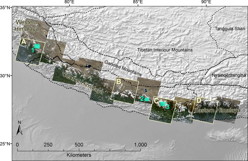
4560                          A. E. Racoviteanu et al.: Surface composition of debris-covered glaciers across the Himalaya

Figure 1. Himalaya study domain showing the large climatic regions from Bolch et al. (2019) as dotted black lines and the studied regions
labelled as western, central and eastern Himalaya. The figure also shows the selected domains across the monsoonal gradient discussed in the
text, shown as light-yellow outlines and labelled as follows: A, Lahaul–Spiti in the monsoon-arid transition zone of the western Himalaya;
B, Manaslu; C, Khumbu and parts of eastern Tibet in the central Himalaya; D, Bhutan in the eastern Himalaya. Turquoise boxes represent
the pond validation sites: 1, Lahaul–Spiti glaciers; 2, Langtang glaciers; 3, Khumbu glaciers. Image footprints are the true colour composite
of Landsat 8 OLI (bands 4,3,2) scenes used in this study and described in Table 1.

domain”, although it also includes glaciers north of the di-                To examine and highlight regional differences in the
vide (Fig. 2). Glaciers in the Khumbu region have been well              composition of the debris-covered surfaces, we use four
studied in terms of glacier mass balance using the tradi-                sub-regions selected across monsoonal gradients as de-
tional glaciologic method (Wagnon et al., 2013), the geodetic            fined in the literature, corresponding to the Landsat scenes
method (Bolch et al., 2008; Nuimura et al., 2012; Brun et al.,           (∼ 32 919 km2 ) shown on Fig. 1 (Bookhagen and Burbank,
2017; Bolch et al., 2011; Rieg et al., 2018), energy balance             2010; Thayyen and Gergan, 2010; Barros and Lang, 2003).
models (Rounce and McKinney, 2014; Rounce et al., 2015;                  The Lahaul–Spiti region in the western Himalaya is in the
Kayastha et al., 2000), debris cover characteristics (Iwata et           monsoon-arid transition zone, characterized by monsoon
al., 1980; Watanabe et al., 1986; Nakawo et al., 1999; Iwata             precipitation during the summer and precipitation from the
et al., 2000; Casey et al., 2012; Takeuchi et al., 2000) and sur-        westerlies in the winter (Thayyen and Gergan, 2010). The
face velocity (Quincey et al., 2009). Rates of change of the             Manaslu and Khumbu regions in the central Himalaya, and
debris-covered glacier areas in the Khumbu region vary from              the Bhutan region in the eastern Himalaya, are all under the
−0.12±0.05 % a−1 from 1962 to 2005 (Bolch et al., 2008) to               influence of the Indian summer monsoon, which brings large
−0.27±0.06 % a−1 from 1962 to 2011 (Thakuri et al., 2014).               amounts of precipitation during the summer months (June to
Supraglacial ponds cover ∼ 0.3 % to 7 % of the glacierized               September) (Barros and Lang, 2003; Bookhagen and Bur-
area in the Khumbu region based on high-resolution Pléiades              bank, 2006) (Fig. 1).
data (Watson et al., 2017a; Kneib et al., 2020; Salerno et al.,             To validate the performance of the spectral unmixing as a
2012); ice cliffs cover between 1 % and 9.2 % of the glacier             basis for estimating pond coverage, we used debris-covered
areas (Brun et al., 2018; Watson et al., 2017a; Kneib et al.,            glacier zones at three validation sites (700–1150 km2 ), se-
2020).                                                                   lected across the wider Himalaya domain from the Khumbu,

The Cryosphere, 15, 4557–4588, 2021                                                           https://doi.org/10.5194/tc-15-4557-2021
A. E. Racoviteanu et al.: Surface composition of debris-covered glaciers across the Himalaya 4561
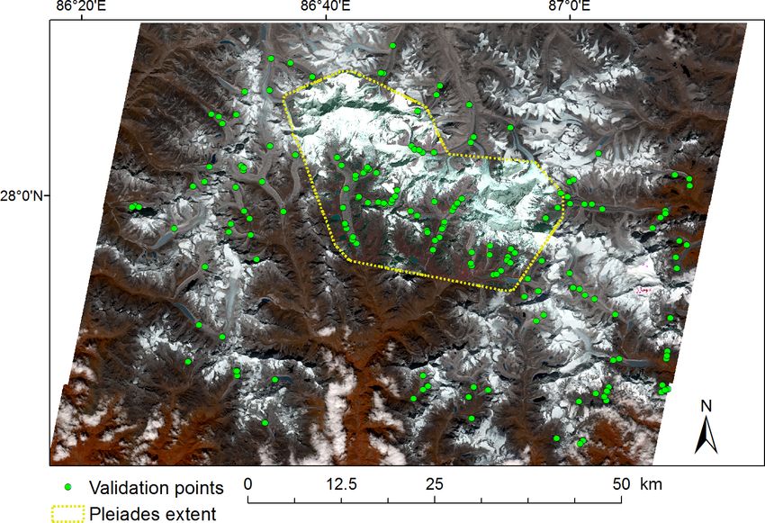
Figure 2. The reference Khumbu domain in Nepal showing the RapidEye image of 9 October 2015 (bands 5, 4 and 3) and the Pléiades image
of 7, 19 and 20 October 2015 (bands 4, 3 and 2) (yellow dotted outline). Vegetation appears in dark red/brown; ponds display various shades
of turquoise. Green dots represent the ground truth points digitized on the high-resolution images and used for the accuracy assessment of
the linear spectral unmixing.
Langtang and Lahaul–Spiti regions (Fig. 1). Supraglacial the 2015 images had too much cloud or snow, we selected
ponds on these glaciers were mapped using OBIA methods images for the same season in 2014 and 2016 (Table 1).
on high-resolution imagery (Sect. 2.6). We acknowledge that this choice may introduce some un-
certainties due to the temporal difference, which we discuss
2.2 Remote sensing data later (Sect. 4.6). The Landsat 8 OLI scene from the Khumbu
domain (30 September 2015) was chosen as reference for
The satellite data used for spectral unmixing comprise of method development and testing. We also performed a sec-
13 Landsat 8 OLI images covering the Himalaya domain ond spectral unmixing on an additional 2016 Landsat 8 OLI
(Fig. 1 and Table 1). Characteristics of these images are scene for the Lahaul–Spiti domain in the western Himalaya
given in Table 1. These were top-of-atmosphere registered, (Table 1) in order to have an analysis that was coincident
radiometrically calibrated and orthorectified imagery (level with the high-resolution data used to validate the supraglacial
L1TP -T1), available at 30 m spatial resolution in the visi- pond mapping within this region.
ble to short-wave infrared since 2013 (Wulder et al., 2019; For calibration and validation of the spectral unmixing
USGS, 2015). We selected scenes from the post-monsoon products at specific locations, we used a combination of high-
period only (September to November) in order to minimize resolution optical imagery from Pléiades and Planet (Ta-
cloud and snow cover occurrence (Bookhagen and Burbank, ble 1). The Pléiades 1A satellite sensor acquires tri-stereo
2006). In addition, Landsat scenes across the domain were high-resolution data (0.5 m spatial resolution in the panchro-
selected around the same date as much as possible to mini- matic band and 2 m in the multispectral bands, blue to near-
mize seasonal differences in surface conditions, notably sea- infrared), with 20 km image swath at nadir (Table 1). Three
sonal changes in pond occurrence (Miles et al., 2017b). All Pléiades scenes from 2015 (7, 19 and 20 October) covered
chosen images were acquired around the same time of the the north, north-east, and south-east parts of the Khumbu
day (05:00 UTC time), with similar solar azimuth (∼ 143◦ ) domain (Fig. 1) (Rieg et al., 2018) and offered the closest
and zenith angle (∼ 30◦ ). This is important in order to ensure match to the date of the reference Landsat image (30 Septem-
that differences in surface conditions were minimal. Where ber 2015); these Pléiades scenes were cloud-free and snow-
https://doi.org/10.5194/tc-15-4557-2021 The Cryosphere, 15, 4557–4588, 2021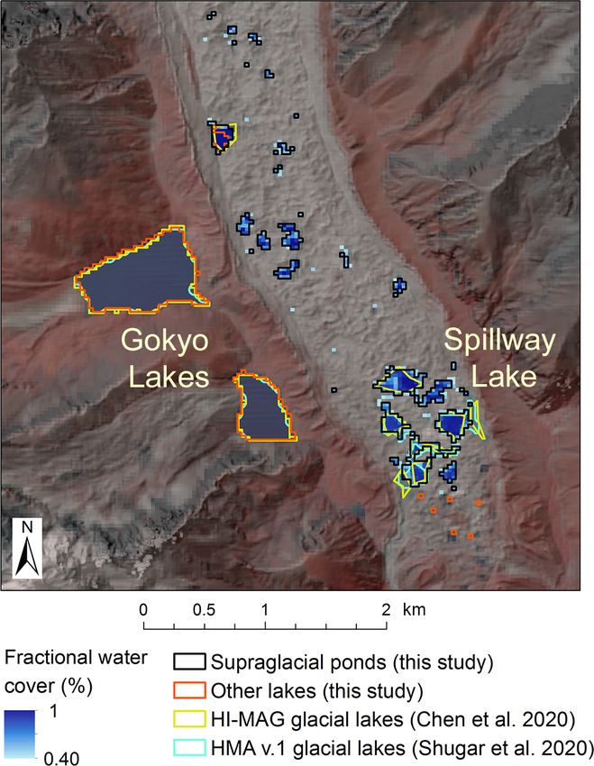
4562                           A. E. Racoviteanu et al.: Surface composition of debris-covered glaciers across the Himalaya

Table 1. Satellite imagery used in this study.

 Sensor            Path/row    Product     Date          Bands                  Cell size (m)   Swath width (km)   Usage
                   137/41                  25 Nov 2014   Band 1 Visible
                   138/41                  19 Nov 2015   0.43–0.45 µm
                   139/41                  9 Oct 2015    Band 2 Visible
                   140/41                  30 Sep 2015   0.450–0.51 µm
                   141/40                  7 Oct 2015    Band 3 Visible
                   142/40                  1 Nov 2016    0.53–0.59 µm
                   143/40                  5 Oct 2015    Band 4 Red
 Landsat 8 OLI                 L1TPT1                                           30              185                Spectral unmixing
                   144/39                  10 Sep 2015   0.64–0.67 µm
                   145/39                  3 Oct 2015    Band 5 Near-IR
                   146/38                  8 Sep 2015    0.85–0.88 µm
                   147/37                  15 Sep 2015   Band 6 SWIR 1
                   147/38                  15 Sep 2015   1.57–1.65 µm
                   147/38                  19 Oct 2016   Band 7 SWIR 2
                                                         2.11–2.29 µm
                                           7 Oct 2015    Blue 430–550 nm                                           Visual checking of
                                           19 Oct 2015   Green 490–610 nm                                          Landsat endmembers;
 Pléiades          –           Level 1A                                         2               20
                                           20 Oct 2015   Red 600–720 nm                                            pond validation
                                                         Near IR 750–950 nm                                        (Khumbu area)
                                                         Green 520–590 nm                                          Visual checking of
                                                         Red 630–685 nm                                            Landsat endmembers
 RapidEye                      Level 3A    9 Oct 2015                           5               77
                                                         Red edge 690–730 nm                                       (Khumbu area)
                                                         Near-IR 760–850 nm
                                           19 Oct 2016   Blue 455–515 nm                                           Additional pond
                                           20 Oct 2016   Green 500–590 nm                                          validation (Lahaul–
 PlanetScope                   Level 3A                                         3               24.6 × 16.4
                                                         Red 590–670 nm                                            Spiti area)
                                                         Near IR 780–860 nm

free over the debris-covered part of the glaciers. The scenes         of Optically Sensed Images and Correlation (COSI-Corr)
were provided as three sets of triplets of primary data (1A)          routine (Leprince et al., 2007) implemented in ENVI 5.5
and were orthorectified in the Leica Photogrammetry Suite             Classic (L3Harris Geospatial, Boulder CO). For the Pléi-
in ERDAS Imagine 2013 (ERDAS, 2010) using the Pléi-                   ades image, after co-registration with 20 tie points and a
ades Rational Polynomial Coefficient model and the Pléiades           second-order polynomial transformation (RMSE = 1.3 m),
DEM (1 m) previously generated using semi-global match-               image displacements were −0.16 m in the E/W direction and
ing (Rieg et al., 2018). The individual image scenes were             0.12 m in the N/S direction. The Planet RapidEye and Plan-
mosaicked to a single image using nearest neighbour at 2 m            etScope scenes were co-registered on the Landsat 8 OLI with
spatial resolution. In addition, a RapidEye level 3A analytic         15 and 10 tie points (RMSE = 5 and 1.6 m, respectively),
ortho-tile from 9 October 2015 from Planet (Planet Team,              yielding offsets of ∼ 1.1 to 1.7 m in the E/W direction and
2017) was used in addition to Pléiades in the Khumbu do-              0.09 to 0.5 m in the N/S direction after co-registration. These
main in order to cover a wider region to better overlap the           offsets were below the spatial resolution of all scenes (2–
Landsat scene. This RapidEye scene consists of orthorecti-            5 m).
fied, surface reflectance data at 5 m spatial resolution and five
multispectral bands, projected to UTM coordinates. A Plan-            2.3     Atmospheric and topographic corrections
etScope ortho-tile from 19 October 2016 (3 m spatial reso-
lution, 4 multi-spectral bands) was used in the Lahaul–Spiti          All Landsat 8 OLI scenes were corrected to minimize at-
area to validate the ponds resulting from unmixing the 2016           mospheric effects due to scattering or absorption from at-
Landsat 8 scene for this region (Table 1). Both RapidEye and          mospheric gases, aerosols and clouds. We used the open-
PlanetScope tiles obtained from Planet were mosaicked to              source Atmospheric and Radiometric Correction of Satellite
single scenes using nearest neighbour. These have a stated            Imagery (ARCSI v 3.1.6) routine based on the 6S algorithm
positional accuracy of < 10 m, reported as root mean square           (Vermote et al., 1997). We applied the STDSREF option in
error, RMSE (Planet Labs, 2021).                                      ARCSI with the shadow option, which provided standardized
   We co-registered all high-resolution images and the cor-           surface reflectance products for all the scenes; deep shadows
responding Landsat 8 OLI images using the Co-registration             were masked out as NoData. ARCSI allows for global and

The Cryosphere, 15, 4557–4588, 2021                                                         https://doi.org/10.5194/tc-15-4557-2021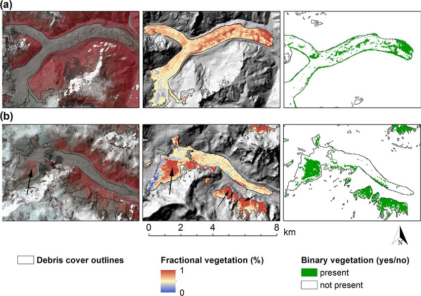
A. E. Racoviteanu et al.: Surface composition of debris-covered glaciers across the Himalaya                               4563

local viewing and solar geometries using physically based il-     “holes” in this dataset. This caused “NULL geometry” errors
lumination and reflectance corrections based on topographic       due to unclosed polygons, duplicated vertices, etc. We fixed
data (Shepherd and Dymond, 2003), a specified atmospheric         these errors in the SDC polygons using the Repair Geome-
profile, an aerosol optical thickness (AOT) value and sensor      try command in ArcGIS v10.8., in order to “fill” the holes
geometry. These settings are important for minimizing dif-        so that these were included in the SDC polygons. For the test
ferences in surface conditions among the various scenes. The      Khumbu area, we removed supraglacial debris polygons with
AOT value was automatically derived in ARCSI by a numer-          an area less than 0.01 km2 , which proved to be erroneous ar-
ical inversion of the surface reflectance on an image basis us-   eas upon visual examination, i.e. sliver polygons or isolated
ing the simple dark object subtraction technique (DOS) from       bare land pixels. Such unwanted small polygons typically re-
the blue band, yielding an AOT of 0.05 for the 30 Septem-         sult from polygon overlays and do not represent a physical
ber 2015 Khumbu scene. To validate the performance of the         entity on the ground (Delafontaine et al., 2009).
DOS technique for the atmospheric profile representation in
our study area for this date, we validated the estimated AOT      2.5   Spectral unmixing background and set-up
against level 1.5 data at reference wavelength of λ = 500 nm
aerosol size from AERONET (https://aeronet.gsfc.nasa.gov/,        In remote sensing, the reflectance spectrum of any image
last access: 20 September 2021) (Giles et al., 2019) and          pixel represents an average of the materials on the ground,
against daily forecast global reanalysis of total optical depth   present in various proportions within that pixel (Keshava and
at multiple wavelengths from the Copernicus Atmospheric           Mustard, 2002). These “mixed pixels” are a common oc-
Monitoring Service (CAMS) (https://atmosphere.copernicus.         currence and are especially a concern in low- to medium-
eu/catalogue#/, last access: 20 September 2021). The AOT          resolution imagery, including Landsat. In the case of debris-
values obtained using the DOS method (0.05) were consis-          covered glacier tongues, constituent materials include vari-
tent with the ones calculated from AERONET and CAMS               ous types of rock debris and/or ice cliffs, supraglacial ponds,
(0.07 and 0.05, respectively). In the Himalaya, we can gen-       and vegetation in various proportions (Rounce et al., 2018).
erally assume relatively clean atmospheres and thus consider      Spectral unmixing techniques serve to quantify mixed spec-
that low AOT values are reasonable (Peter Bunting, Aberys-        tra and to decompose each pixel into its constituent ma-
twyth University, personal communication, February 2021).         terials based on their characteristic, distinct spectral signa-
Our choice of a constant AOT value in high environments is        tures. These materials are referred to as “pure” endmembers
in line with findings from other studies (Gillingham et al.,      (Painter et al., 2009; Keshava and Mustard, 2002) and are ei-
2013; Matta et al., 2017). Surface topography used for the        ther extracted from the image itself before unmixing using
atmospheric and topographic corrections was based on the          unsupervised techniques or supplied by the user using a pri-
ALOS Global Digital Surface Model (AW3D30 version 2.2,            ori knowledge (Painter et al., 2009; Keshava and Mustard,
at 30 m) (JAXA, 2019), constructed from data acquired from        2002; Dixit and Agarwal, 2021). The relationship between
2006 to 2011. The vertical accuracy of ∼ 10 m in eastern          the fractional abundance of each material and its spectra is
Nepal (Tadono et al., 2014) is superior to that of Shuttle        most often defined as a linear combination of the spectral re-
Radar Topography Mission (SRTM) DEM (23.5 m, reported             flectance of the distinct constituent materials. This is imple-
by Mukul et al., 2017), because it contains fewer data voids      mented as linear mixing models (LMMs), used for example
and provides better shadow rendering in our area.                 to distinguish among vegetation, rock or different snow grain
                                                                  sizes (Painter et al., 2009). LMMs are easy to implement and
2.4   Supraglacial debris cover data                              are therefore widely used (Dixit and Agarwal, 2021; Keshava
                                                                  and Mustard, 2002). In contrast, nonlinear mixing models
In this study, we constrained our analysis over supraglacial      take into account multiple scattering between surfaces and
debris surfaces, extracted from the database of global distri-    are used in forested areas where canopy height or particu-
bution of supraglacial debris cover (Scherler et al., 2018) and   late mineral mixtures are in close association (Roberts et al.,
referred to hereinafter as the “SDC”. Debris-covered glacier      1993). They are more realistic but are also more difficult to
outlines in this dataset were derived from Landsat 8 OLI          implement (Dixit and Agarwal, 2021).
and Sentinel-2 data using automated approaches on Google             To yield physically meaningful results, fractions obtained
Earth Engine by excluding clean ice and snow from glacier         from spectral unmixing should ideally comply with two ma-
areas within the limits of the Randolph Glacier Inventory         jor constraints: (a) the non-negativity (or positivity) con-
(RGI v.6) (RGI Consortium, 2017). Outlines span the pe-           straint (i.e. fractions should not be negative) and (b) the sum
riod 1998 to 2001 for the central and eastern Himalaya, the       to unity (i.e. for each pixel, fractions should add up to 1)
year 2002 for the western Himalaya (monsoon-dry transi-           (Keshava and Mustard, 2002). The non-negativity condition
tion zone) and mostly the year 2010 for glaciers in China.        is recommended because negative reflectance values have no
In this study, the outlines obtained from the SDC dataset         physical meaning, and the sum-to-unity constraint is recom-
required pre-processing because supraglacial ponds along          mended when very dark endmembers such as shadows are
with other surfaces such as nunataks were represented as          targeted or for unmixing radiance or thermal infrared emis-

https://doi.org/10.5194/tc-15-4557-2021                                                The Cryosphere, 15, 4557–4588, 2021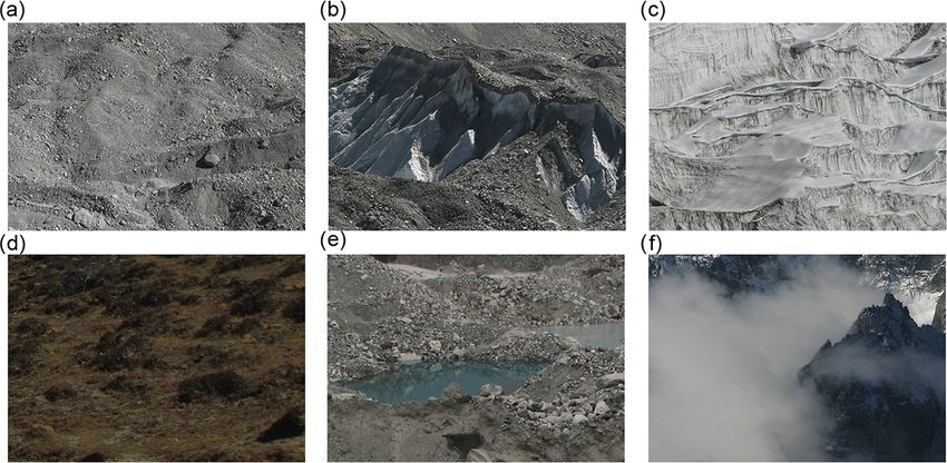
4564                         A. E. Racoviteanu et al.: Surface composition of debris-covered glaciers across the Himalaya

sivity. Models that comply with both conditions (called “fully      (Naegeli et al., 2015, 2017; Casey and Kääb, 2012). To min-
constrained models”) are difficult to achieve because they re-      imize the number of endmembers, we made several choices:
quire perfect knowledge of the system, which is rarely feasi-
ble. Furthermore, fully constrained models have been shown           (a) We did not consider snow separately from ice.
to produce unrealistic fractions in poorly defined areas or ar-     (b) We assumed the supraglacial ponds to be mostly of tur-
eas of low illumination (Cortés et al., 2014). In this study, we        bid type, i.e. those containing larger quantities of sus-
applied a LMM with endmembers extracted from the Land-                  pended sediments. We based this choice on results from
sat 8 OLI image itself, and we constrained our analysis over            Matta et al. (2017), who reported 52 % of ponds in the
the supraglacial debris cover only to reduce model complex-             Himalaya to have grey waters and 24 % blueish waters;
ity. We used the LMM implementation in the ENVI 5.5 soft-               the water spectra in Fig. 4a corresponds well with field-
ware (L3Harris Geospatial, Boulder CO).                                 based spectra for other turbid lakes in the Khumbu re-
                                                                        gion, such as Chola Lake, reported in their study.
2.5.1   Endmember selection and spectral signatures
                                                                     (c) Based on our field observations of high-altitude vege-
                                                                         tation in the Khumbu region (Fig. 3d), we defined the
The selection of endmembers is crucial in determining the                vegetation endmember as “dry vegetation”, whose spec-
accuracy and reliability of the spectral unmixing (Song,                 tral signature (a) corresponds roughly to the graminoid
2005; Dixit and Agarwal, 2021), and it requires some                     shrubs or overgrown vegetation with a grass-like ap-
trial and error as well as a priori knowledge. We selected               pearance typically found at high altitudes (Wehn et al.,
the endmembers within the debris-covered areas in the                    2014).
Khumbu domain, based on the reference Landsat 8 OLI
scene (30 September 2015). Prior to this, we performed a            (d) Prior to the unmixing, we removed deep shadows during
forward minimum noise fraction transform on the Landsat                 the topographic corrections with ARCSI and assigned
scene (Green et al., 1988), which consists of a linear trans-           them to NoData so they were not considered an end-
formation of the data based on principal component analysis             member.
and allowed us to estimate noise in the bands. All bands had        We ran the LMM for various combinations and numbers
eigenvalues > 1, so we determined the dimensionality of the         of endmembers (three to six endmembers) and recorded the
Landsat data as n = 7. We used the unsupervised pixel purity        model RMSE for each combination. We examined the resid-
index routine in ENVI to find pure pixels in an automated           uals (RMSE band) provided from the unmixing to determine
manner. This routine outputs a data cloud where the value           areas of missing or incorrect endmembers; when this con-
of each point indicates the number of times each pixel was          tained distinct features, it indicated poorly defined endmem-
marked as extreme, thus representing pixels with the highest        bers. We excluded the endmembers one by one and ran the
occurrence in the image. We optimized the pure pixel extrac-        LMM until we obtained a residual speckle noise, also known
tion using various numbers of iterations (20 000 to 50 000)         as a “salt and pepper” effect, with no distinct features, indi-
with thresholds ranging from 2 to 3 (i.e. 2 to 3 times the          cating that no endmembers were missing or misidentified.
noise level in the data) until all pure pixels were detected.
Larger thresholds identify more extreme pixels, but they are        2.5.2   Surface classification from fractional maps
less likely to be pure endmembers. Pure pixels were identi-
fied on the Landsat 8 OLI scene as corresponding to six sur-        LMM routines result in a multi-band raster containing pixel-
face types: clean ice, dry vegetation, clouds, light debris, dark   by-pixel fractional cover values for each class, which ideally
debris and turbid water (Fig. 3). These were checked against        range from 0 to 1. When we obtained negative values for a
co-registered Pléiades and RapidEye false colour composites         class, we assumed that the material was missing and forced
in the Khumbu region in order to minimize any occurrence            these values to zero. Positive values were normalized by di-
of mixed pixels.                                                    viding each endmember fraction by the sum of the endmem-
   The spectra of the six endmembers (Fig. 4a) were statis-         bers, so that the sum of the fractions of the various materials
tically separable based on the Jeffries–Matusita and trans-         in each pixel added up to 1. This is a common procedure
formed divergence separability measures (Richards, 2013)            suggested by previous studies (Rosenthal and Dozier, 1996;
(values > 1.9–2.0). We defined both light and dark de-              Quintano et al., 2012; Cortés et al., 2014) when the sum-to-
bris endmembers on the basis of their spectral differences          one condition is not satisfied.
(Fig. 4a), also noted in other studies (Casey et al., 2012;            For further analysis, we require maps of the surfaces rather
Kneib et al., 2020). We visually compared these spectral sig-       than just a numerical value of area, so we classified the 30 m
natures with those we acquired previously in the field on Mer       fractional maps by applying a threshold α to produce bi-
de Glace (French Alps) using an SVC HR-1024 spectrometer            nary maps for each class. Previous studies used a minimum
(350 to 2500 nm) (Racoviteanu and Arnaud, 2013) (Fig. 4b),          threshold of α = 0.4 or 0.5; i.e. a pixel was assigned to a
as well as with supraglacial debris spectra from other papers       class if it contained a fraction of 40 %–50 % to 100 % of that

The Cryosphere, 15, 4557–4588, 2021                                                    https://doi.org/10.5194/tc-15-4557-2021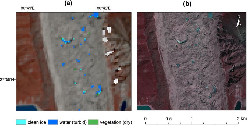
A. E. Racoviteanu et al.: Surface composition of debris-covered glaciers across the Himalaya                                                    4565

Figure 3. Types of surfaces present in the study area: (a) light debris cover (quartz, feldspar); (b) darker schistic debris with ice cliff; (c) clean
ice with crevasses in the glacier ablation area; (d) graminoid shrub type vegetation (dry); (e) supraglacial lakes with different turbidity levels;
(f) valley clouds. All photos were taken in the Khumbu region. Photo credit: Adina E. Racoviteanu.

                                                                             constituent material (Hall et al., 2002). The thresholds vary
                                                                             by class, because any pixel contains a mixture of materials
                                                                             in various proportions (Sect. 3.1). Pixels which satisfy two
                                                                             different thresholds are categorized as “unclassified”. For the
                                                                             supraglacial ponds in the Khumbu domain, we defined the
                                                                             water threshold quantitatively based on comparison of the
                                                                             LMM-derived pond areas against those derived from Pléi-
                                                                             ades for seven glaciers (Sect. 2.6), and we evaluated the sen-
                                                                             sitivity of the chosen water threshold. For the other classes,
                                                                             the thresholds were adjusted carefully based on visual inter-
                                                                             pretation against the Pléiades and RapidEye images in the
                                                                             Khumbu domain. The thresholds established for the Khumbu
                                                                             region were applied over the entire Himalaya domain.

                                                                             2.5.3    Accuracy assessment

                                                                             The performance of the LMM was assessed both qualita-
                                                                             tively (on the basis of visual interpretation and compari-
                                                                             son with surfaces visible on the high-resolution Pléiades and
                                                                             RapidEye) and quantitatively (using established measures,
                                                                             i.e. RMSE, fractional value abnormalities and the residual
                                                                             band output in the LMM) (Gillespie et al., 1990). To quanti-
                                                                             tatively assess the ground accuracy of the LMM, we manu-
Figure 4. (a) Spectral signatures of endmembers extracted from               ally digitized 151 test pixels covering all six classes (10–38
Landsat 8 OLI bands 1 to 7 (30 September 2015 Khumbu image)                  pixels per class) on false colour composites of the Pléiades
after the atmospheric and topographic corrections; (b) field spec-           and RapidEye images in the Khumbu domain using a simple
tra from the debris-covered part of Mer de Glace Glacier (France)            random sampling strategy. The reference points were chosen
shown for comparison purposes only.                                          so that they were well distributed across the Khumbu domain
                                                                             (Fig. 2) and were taken to represent ground truth. The pre-
                                                                             dicted class was compared to the ground truth at each pixel

https://doi.org/10.5194/tc-15-4557-2021                                                               The Cryosphere, 15, 4557–4588, 2021
4566                         A. E. Racoviteanu et al.: Surface composition of debris-covered glaciers across the Himalaya

to generate a confusion matrix and to compute the overall           prevent over-segmenting and to combine different segments
accuracy of the model (percent pixels classified correctly).        into single ponds. The resulting polygons were further man-
We also report class-specific metrics as true positives (num-       ually corrected (split, merged or digitized) for any missing
ber of pixels correctly classified and found in a class, TP),       and/or shaded areas beneath ice cliffs as described in Watson
true negatives (number of correctly classified pixels that do       et al. (2017a). Our aim was not to construct a sophisticated
not belong to a class, TN), false positives (number of pixels       OBIA classification scheme but rather to use the feature ex-
that were incorrectly assigned to a class, FP) and false nega-      traction module as a time-saving strategy and to add objec-
tives (number of pixels that were omitted from a class, FN).        tivity to the manual digitization.
We calculated three metrics which are suitable for multi-class
classification routines (Sokolova and Lapalme, 2009) as fol-        2.7    Auxiliary region-wide datasets
lows (Eqs. 1–3):
                                                                    We explored the dependency of the resulting supraglacial
               TP                                                   pond cover incidence on topographic variables: elevation
Precision =          ,                                       (1)
             TP + FP                                                bands above the termini, slope and aspect of the debris cover
             TP                                                     areas. These were calculated over the debris-covered parts
Recall =          ,                                          (2)
          TP + FN                                                   of the glaciers on the basis of the AW3D30 DEM (30 m).
                2TP                                                 Only glacier polygons with area larger than 1 km2 , result-
F score =                .                                   (3)    ing in a subset of 408 glaciers, were selected from the SDC
           2TP + FP + FN
                                                                    database over the Himalaya domain for an in-depth glacier-
Precision measures the agreement between ground data and            by-glacier analysis. The area threshold was applied in order
classified data, i.e. the probability that a pixel classified as    to remove spurious small bare land patches or isolated debris
water is indeed water on the ground. Recall measures the ef-        pixels present in the SDC database. While the vast majority
fectiveness of the classifier to identify a pixel in the class of   of glaciers in the Himalaya are smaller than 1 km2 , these are
interest, i.e. the percentage of results correctly classified by    mostly clean glaciers (Racoviteanu et al., 2015). In addition
the algorithm. F score balances precision and recall as the         to the glacier-by-glacier basis analysis, we also binned the
harmonic means of the two and measures the relation be-             topographic variables, i.e. 100 m elevation, 2◦ slope and 45◦
tween the pixels on the ground and those classified, i.e. the       aspect, and summarized the pond incidence in each bin.
model accuracy for each class. For all metrics, a poor score           We explored spatial patterns in the pond incidence and
is 0.0 and a perfect score is 1.0.                                  supraglacial vegetation with respect to regional climate gra-
                                                                    dients, average glacier mass balance and average surface
2.6    Validation of supraglacial ponds with
                                                                    velocity. Climate data (total precipitation and average tem-
       high-resolution data
                                                                    perature) were obtained from ERA5-Land, which provides
We validated the performance of the spectral unmixing for           gridded monthly average means at 0.1◦ × 0.1◦ of land sur-
supraglacial pond areas on the basis of high-resolution im-         face properties (Muñoz-Sabater, 2019). Gridded glacier ele-
agery for 6 to 7 debris-covered glacier extents at each of the      vation change data at 30 m resolution for the period 2000–
three sites shown in Fig. 1. For the Khumbu and Lahaul–Spiti        2019 were obtained from Shean et al. (2020). Glacier surface
glaciers, supraglacial pond areas were mapped from Pléi-            velocities for the period 2013–2015 based on Landsat data
ades and PlanetScope imagery, respectively (Table 1), using         were obtained from Dehecq et al. (2015). All topo-climatic
OBIA techniques (Blaschke et al., 2014) implemented in the          variables were binned and averaged over a 1◦ × 1◦ grid as
ENVI Feature Extraction Module (Harris Geospatial, 2017).           in other studies (e.g. Brun et al., 2017; Dehecq et al., 2019)
In the Khumbu region, the Pléiades images were acquired             to explore the topo-climatic controls on pond and vegetation
several weeks apart from the date of the Landsat scene in           incidence.
some parts of the region (see Table 1), but we assume min-
imal lateral expansion between the two dates, as discussed          3     Results
by Watson et al. (2018). For the Langtang region, we vali-
dated our LMM-derived pond areas with those reported for            3.1    Fractional maps
seven glaciers based on SPOT7 satellite imagery in Steiner
et al. (2019). The OBIA method used for the Khumbu and              Here we present results of the unconstrained LMM, because
Lahaul–Spiti regions consisted in a segmentation-only ex-           this had a lower RMSE (0.6 %) compared to the partially con-
traction workflow on the visible bands of Pléiades and/or           strained model run (RMSE of 1.5 %). The normalized frac-
PlanetScope, with an edge algorithm (to delineate the pond          tional maps of the six surface types are presented in Fig. 5;
segments), a fast lambda setting (to merge adjacent segments        fractional values ranged from 0.004 to 1. Fractional water
with similar colours and borders) and a texture kernel size         values greater than 0.5 correspond to supraglacial ponds, vis-
of 3 pixels (suitable for segmenting small areas). The scale        ible for example at the termini of Ngozumpa and Khumbu
and merge levels were adjusted against colour composites to         glaciers (Fig. 6a and b). Light debris and dark debris were

The Cryosphere, 15, 4557–4588, 2021                                                    https://doi.org/10.5194/tc-15-4557-2021
A. E. Racoviteanu et al.: Surface composition of debris-covered glaciers across the Himalaya 4567
Figure 5. Fractional maps obtained from the LMM routine for a subset of the Khumbu region. Colour bars show the percentage covered by
each type of material on a pixel-by-pixel basis: (a) clean ice; (b) turbid water; (c) dark debris; (d) light debris; (e) clouds; (f) dry vegetation.
identified with a threshold of 0.25 and 0.40, respectively, de- ing, with an F score of ∼ 0.7 and lower precision score for
fined visually on the basis of the Pléiades image. Dry vegeta- dark debris (0.56) compared to light debris (0.72) (Table 2).
tion patches generally exhibited pixel fractions greater than This suggests that in the case of dark debris, the LMM model
0.65. Pixels with abnormally high positive fractional vegeta- was less accurate than light debris, because pixels from other
tion values were found in areas of healthy green vegetation classes (clean ice, water and light debris) got mistakenly as-
and/or bare terrain, which should not be part of the debris- signed to this class. Clouds were classified with low preci-
covered tongues, as will be discussed later (Sect. 4.5). Cloud sion and low recall scores (F score of ∼ 0.5), which means
pixels display fractional values greater than 0.45, although that the LMM performed relatively poorly for this class and
some pixels were mixed with debris, particularly at cloud it also missed 50 % of the cloud pixels. There was confu-
shadow areas. For clean ice, fractional values were rather low sion between clean ice and cloud pixels, i.e. clean ice pixels
(0.20) and ranged from 0 (areas which might have some de- were mistakenly included in the cloud class. Clean ice was
gree of dirty, dark ice with a lower albedo) to 1 (small number the most poorly classified, with a recall score close to 0 and
of clean ice pixels found in the upper areas of supraglacial F score of 0.13; one ice pixel was correctly identified, but
debris). other surfaces were confounded with ice. We attribute this
to the poorly defined ice class in the model data (i.e. lim-
3.2 Accuracy of the LMM-based classification for the ited number of pure ice pixels used to extract the spectral
Khumbu region signature). Based on these measures, we note that overall
the LMM most accurately classified the water and vegeta-
Accuracy measures presented in Table 2 for the Khumbu do- tion classes, with reasonable performance for the light de-
main show that errors were not evenly distributed among bris class but poor performance for clean ice and clouds. The
classes. For the water and vegetation classes, recall score overall accuracy of the LMM-based classification of the six
was 0.83 to 0.84, respectively, with a precision of 0.94 and surfaces was 75 %; however, this is a rather coarse metric,
0.93, respectively (Table 2). For these classes, the LMM and it does not indicate the specific performance of the model
achieved a balance of precision and recall metrics, with a for each class, so we do not use this here as evaluation of the
high F score of ∼ 0.9 indicating an accurate model. For the accuracy.
debris classes, the model was reasonable but not outstand-
https://doi.org/10.5194/tc-15-4557-2021 The Cryosphere, 15, 4557–4588, 20214568 A. E. Racoviteanu et al.: Surface composition of debris-covered glaciers across the Himalaya
Table 2. Summary of accuracy metrics per class for the Khumbu region, calculated based on the confusion matrix, including true positives
(TP), false positives (FP), false negatives (FN) and true negatives (TN).
Class TP FP FN TN Recall Precision F score
Clean ice 1 0 13 112 0.07 1.00 0.13
Water (turbid) 32 2 6 81 0.84 0.94 0.89
Debris (dark) 29 23 0 84 1.00 0.56 0.72
Debris (light) 21 8 9 62 0.70 0.72 0.71
Clouds 5 3 5 92 0.50 0.63 0.56
Vegetation (dry) 25 2 5 88 0.83 0.93 0.88
Table 3. Sensitivity analysis of the supraglacial pond area for the
seven reference glaciers in the Khumbu domain, obtained using var-
ious thresholds applied to the fractional water maps.
Glacier Surface area (km2 )
Fractional Fractional Fractional
water water water
> 0.4 > 0.45 > 0.5
Khumbu 0.45 0.32 0.20
Lhotse 0.07 0.06 0.05
Lhotse Nup 0.03 0.03 0.02
Ngozumpa 0.79 0.66 0.50
Nuptse 0.09 0.05 0.03
Changri Nup 0.25 0.19 0.09
Gaunara 0.16 0.12 0.07
Total pond coverage 1.8 1.4 1.0
3.3 Supraglacial pond thresholds and validation
The sensitivity analysis of the pond areas obtained from
LMM fractional maps with various thresholds (Table 3) in-
dicates that there was up to 40 % variability in total pond
area when compared to Pléiades-based ponds, depending
on the glacier. A threshold of 0.5 applied to the water
class (fractional water > 0.5 = supraglacial ponds) yielded
the best agreement with the total pond areas for the seven
glaciers, obtained from OBIA mapping on the Pléiades im-
age (1.0 km2 compared to 1.1 km2 for the total coverage, re-
spectively, or a 9 % difference) (Table 4). For the Khumbu
Glacier, LMM with a threshold of 0.5 yielded a pond area of
0.20 km2 versus 0.23 km2 from Pléiades (Table 4), which is
in agreement with the area reported by Watson et al. (2017b)
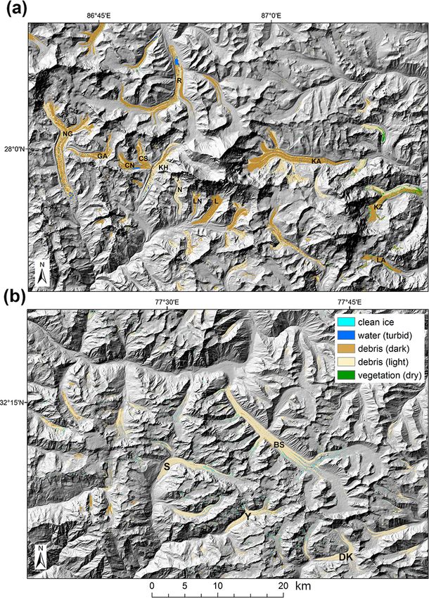
Figure 6. Comparison of the Landsat sub-pixel classified fractional
(0.24 km2 ) using the same Pléiades image (7 October 2015).
ponds (dark blue) with OBIA pond outlines (light blue) based on
In the Lahaul–Spiti region, for the seven glaciers we inves-
high-resolution data for the termini of three glaciers: (a) Ngozumpa
Glacier, (b) Khumbu Glacier and (c) Bara Shigri Glacier. The back- tigated, LMM yielded a total pond area of 0.14 km2 (0.31 %
ground images are colour composites (bands 1,2,3) of Pléiades im- of the total debris-covered area of the glaciers). The area
agery (a, b) and PlanetScope imagery (c). Glacier outlines are from mapped from PlanetScope image from the same date (19 Oc-
the SDC dataset (Scherler et al., 2018). tober 2016) using OBIA yielded 0.10 km2 (0.22 % of the
debris-covered area) (Table 4).
In the Langtang region, for the six glaciers investigated in
Steiner et al. (2019), our LMM-derived pond areas yielded
The Cryosphere, 15, 4557–4588, 2021 https://doi.org/10.5194/tc-15-4557-2021A. E. Racoviteanu et al.: Surface composition of debris-covered glaciers across the Himalaya 4569
Table 4. Validation of the Landsat spectral unmixing for supraglacial pond coverage at selected glaciers at three sites across the Himalaya
domain, shown in Fig. 1.
Region/ Debris area Pond area % Date Pond area % Date
glacier name (km2 ) (km2 ) coverage (km2 ) coverage
Khumbu Landsat 8 spectral unmixing Pléiades OBIA
Khumbu 7.50 0.20 2.80 0.21 2.70
Lhotse 5.20 0.05 0.90 0.08 1.70
Lhotse Nup 1.50 0.02 1.00 0.02 1.60
Ngozumpa 19.40 0.50 2.70 0.59 3.00
30 Sep 2015 7 Oct 2015
Nuptse 2.90 0.03 0.90 0.03 1.00
Changri Nup & Shar 7.30 0.09 1.30 0.11 1.50
Gaunara 5.20 0.07 1.40 0.09 1.70
Total 49.00 1.00 2.04 1.10 2.24
Langtang Landsat 8 spectral unmixing SPOT 7 manual digitization (from Steiner et al., 2019)
Lirung 1.44 0.00 0.00 0.00 2.70
Ghanna 0.69 0.00 0.00 0.00 1.70
Langshisha 4.46 0.01 0.20 0.01 1.60
Langtang 16.17 0.15 0.92 7 Oct 2015 0.18 3.00 6 Oct 2015
Salbhachum 3.44 0.01 0.33 0.02 1.00
Lirung 1.44 0.00 0.00 0.00 1.50
Total 26.20 0.17 0.64 0.21 0.86
Lahaul–Spiti Landsat 8 spectral unmixing PlanetScope OBIA
Yichu 5.7 0.002 0.000 0.001 0.000
Dibi Ka 5.6 0.004 0.000 0.009 0.000
Bara Shigri 21.3 0.126 0.027 0.076 0.016
Sara Umga 7.8 0.007 0.001 0.012 0.001
19 Oct 2016 19 Oct 2016
G077666E32079N 0.7 0.000 0.000 0.000 0.000
G077559E32106N 3.2 0.000 0.000 0.000 0.000
G077698E32078N 1.2 0.001 0.000 0.000 0.000
Total 45.5 0.14 0.31 0.10 0.22
a total of 0.17 km2 pond area (0.64 % of the debris-covered 3.4 Application to regional non-glacier lake databases
area). Steiner et al. (2019) obtained a total pond area of
0.21 km2 (0.86 % of the debris-covered area) for the same While supraglacial ponds are the focus of this study, we
glaciers based on manual digitization by multiple analysts mention that LMMs can also be parameterized to map other
from SPOT7 data for the same date as the Landsat. LMM lakes, by masking the debris-covered glacier areas and re-
underestimated the pond area by 0.05 km2 (19 %), which is placing the turbid water endmember with the clear water end-
within the uncertainty range (21 %) reported for the ponds in member, which has a lower spectral signature (Fig. 4a). This
the Langtang area by Steiner et al. (2019). is beyond the purpose of this study, but we provide an il-
Visually, in the Khumbu region, the spectrally unmixed lustration of such an output for the terminus of Ngozumpa
pond pixels correspond well with the validation dataset Glacier in Fig. 7. We present the ponds and lakes on the de-
(Fig. 6a and b), although there is a difference in the repre- bris cover and outside it for comparison with two existing
sentation of the pond surfaces due to the spatial resolution glacial lake databases constructed from the same year (2015
(30 m Landsat vs. 2 m Pléiades). Similarly, in the Lahaul– Landsat): the HMA v.1 lake dataset, derived using a normal-
Spiti region, locations of the supraglacial ponds correspond ized difference water index (Shugar et al., 2020), and HI-
well between LMM and PlanetScope on Bara Shigri Glacier MAG constructed using a modified NDWI and manual cor-
(Fig. 6c), but the small ponds are not identified using the wa- rections (Chen et al., 2021). A comparison with other global
ter threshold of 0.5, which assumes that more than 50 % of databases such as the Global Surface Water dataset (Pekel et
the pixel area is covered by water. al., 2016) was not undertaken here, as this has already been
shown to underestimate the water occurrence over most of
the Himalaya by Chen et al. (2021). With regards to HMA
v.1 and HI-MAG datasets, Fig. 7 shows that the lake out-
https://doi.org/10.5194/tc-15-4557-2021 The Cryosphere, 15, 4557–4588, 2021You can also read