SPEAD 1.0 - Simulating Plankton Evolution with Adaptive Dynamics in a two-trait continuous fitness landscape applied to the Sargasso Sea
←
→
Page content transcription
If your browser does not render page correctly, please read the page content below
Geosci. Model Dev., 14, 1949–1985, 2021
https://doi.org/10.5194/gmd-14-1949-2021
© Author(s) 2021. This work is distributed under
the Creative Commons Attribution 4.0 License.

SPEAD 1.0 – Simulating Plankton Evolution with Adaptive
Dynamics in a two-trait continuous fitness landscape
applied to the Sargasso Sea
Guillaume Le Gland1 , Sergio M. Vallina2 , S. Lan Smith3 , and Pedro Cermeño1
1 Department  of Marine Biology and Oceanography, Institute of Marine Sciences (ICM – CSIC), Barcelona, Spain
2 Spanish Institute of Oceanography (IEO), Ave Principe de Asturias 70 bis, 33212 Gijón, Spain
3 Earth SURFACE Research Center, Research Institute for Global Change, JAMSTEC, Yokosuka, Japan

Correspondence: Guillaume Le Gland (legland@icm.csic.es)

Received: 9 September 2020 – Discussion started: 27 November 2020
Revised: 2 March 2021 – Accepted: 9 March 2021 – Published: 13 April 2021

Abstract. Diversity plays a key role in the adaptive capacity        ulation are driven by seasonal variations in vertical mixing,
of marine ecosystems to environmental changes. However,              nutrient concentration, water temperature, and solar irradi-
modelling the adaptive dynamics of phytoplankton traits re-          ance. The simulated bulk properties are validated by observa-
mains challenging due to the competitive exclusion of sub-           tions from Bermuda Atlantic Time-series Studies (BATS) in
optimal phenotypes and the complexity of evolutionary pro-           the Sargasso Sea. We find that moderate mutation rates sus-
cesses leading to optimal phenotypes. Trait diffusion (TD) is        tain trait diversity at decadal timescales and soften the almost
a recently developed approach to sustain diversity in plank-         total inter-trait correlation induced by the environment alone,
ton models by introducing mutations, therefore allowing the          without reducing the annual primary production or promot-
adaptive evolution of functional traits to occur at ecological       ing permanently maladapted phenotypes, as occur with high
timescales. In this study, we present a model called Simulat-        mutation rates. As a way to evaluate the performance of the
ing Plankton Evolution with Adaptive Dynamics (SPEAD)                continuous trait approximation, we also compare the solu-
that resolves the eco-evolutionary processes of a multi-trait        tions of SPEAD to the solutions of a classical discrete enti-
plankton community. The SPEAD model can be used to eval-             ties approach, with both approaches including TD as a mech-
uate plankton adaptation to environmental changes at dif-            anism to sustain trait variance. We only find minor discrep-
ferent timescales or address ecological issues affected by           ancies between the continuous model SPEAD and the dis-
adaptive evolution. Phytoplankton phenotypes in SPEAD are            crete model, with the computational cost of SPEAD being
characterized by two traits, the nitrogen half-saturation con-       lower by 2 orders of magnitude. Therefore, SPEAD should
stant and optimal temperature, which can mutate at each gen-         be an ideal eco-evolutionary plankton model to be coupled
eration using the TD mechanism. SPEAD does not resolve               to a general circulation model (GCM) of the global ocean.
the different phenotypes as discrete entities, instead comput-
ing six aggregate properties: total phytoplankton biomass,
the mean value of each trait, trait variances, and the inter-
trait covariance of a single population in a continuous trait        1   Introduction
space. Therefore, SPEAD resolves the dynamics of the pop-
ulation’s continuous trait distribution by solving its statistical   Phytoplankton are a polyphyletic group of microscopic pri-
moments, wherein the variances of trait values represent the         mary producers widespread in aquatic environments. They
diversity of ecotypes. The ecological model is coupled to a          are mainly single-celled, although colonial or multicellular
vertically resolved (1D) physical environment, and therefore         species exist in most phytoplankton phyla (Beardall et al.,
the adaptive dynamics of the simulated phytoplankton pop-            2009). Despite accounting for only 1 % of the global photo-
                                                                     synthetic biomass, phytoplankton perform more than 45 % of

Published by Copernicus Publications on behalf of the European Geosciences Union.
1950 G. Le Gland et al.: SPEAD 1.0 Earth’s net primary production (Field et al., 1998; Falkowski one or several compartments of nutrients, phytoplankton, et al., 2004). They are the basis of all oceanic food webs zooplankton, and detritus (Fasham et al., 1990). Since the and play key roles in biogeochemical cycles (Falkowski, early 1990s (Maier-Reimer, 1993), the increase in computa- 2012). In particular, they have a large impact on global cli- tional power has allowed biogeochemical models to be fully mate through the export of detritic carbon from the sur- coupled with ocean circulation (Aumont et al., 2003; Follows face to the ocean interior, sequestrating carbon in the deep et al., 2007). However, representing all the phytoplankton di- ocean for timescales from a few years to more than a mil- versity in models is neither feasible nor desirable. The com- lennium depending on the depth they reach (DeVries and putational cost would be high, and even if computationally Primeau, 2011; DeVries et al., 2012). This process, called feasible, the existing observations would not suffice to con- the “biological carbon pump”, regulates the concentration of strain the many free parameters. carbon dioxide in the atmosphere (Volk and Hoffert, 1985; Instead, ecological models account for biodiversity Falkowski et al., 1998). through a few key traits representing physiological charac- Phytoplankton are highly diverse and live in many differ- teristics or adaptation to different environments. The most ent environments. They differ in their ecological interactions widely investigated phytoplankton traits are cell size, nutri- and the processes through which they mediate biogeochem- ent niche, optimal temperature, optimal irradiance, and re- ical cycles. For instance, some species can fix atmospheric sistance to predation. Some trait-based models divide the nitrogen and enrich oligotrophic regions; some produce bal- phytoplankton community into discrete entities or “boxes” last minerals (mainly silica and calcium carbonate) and sink with different traits. The boxes can be as simple as diatoms faster to the deep ocean, and others are mixotrophic, being and small phytoplankton groups (Aumont et al., 2015), with able to both photosynthesize and feed on organic sources diatoms having higher nutrient concentration niches, or in- (Le Quéré et al., 2005). Most species are denser than seawa- clude more complex divisions into functional groups (Baretta ter and eventually sink, but some are buoyant (Lännergren, et al., 1995; Le Quéré et al., 2005; Follows et al., 2007). In 1979; Villareal, 1988). Phytoplankton size ranges from less this article, we will call these models “discrete” or “multi- than 1 µm for cyanobacteria like Prochlorococcus (Chisholm phenotype”. The other approach, which further reduces the et al., 1988) to more than 1 mm for the giant diatom Eth- number of equations while still allowing communities to modiscus rex (Swift, 1973; Villareal and Carpenter, 1994). adapt to changes in their environments, is to consider one or Their half-saturation constants for the main limiting nu- several continuously distributed traits and to compute only trients range over 3 orders of magnitude (Edwards et al., the dynamics of aggregate properties, such as community 2012), reflecting adaptation to different nutrient supply lev- biomass, mean trait values, and trait variances (Wirtz and els. They are also adapted to very different temperatures: Eckhardt, 1996; Norberg et al., 2001; Bruggeman and Kooij- some diatoms can grow within sea ice (Ackley and Sullivan, man, 2007; Merico et al., 2009; Acevedo-Trejos et al., 2016; 1994), whereas some hyperthermophilic cyanobacteria can Smith et al., 2016; Chen and Smith, 2018). In this method grow at up to 75 ◦ C in hot springs (Castenholz, 1969). Most trait variance can be used as a quantitative index of biodiver- oceanic species have an optimal temperature for growth be- sity. A community with a higher trait variance is considered tween 0 and 35 ◦ C (Thomas et al., 2012). Even within the to be more diverse because it has a wider spread and more same species or genus, wide variability has been observed even distribution of trait values (Li, 1997), although it does for key traits such as iron requirements (Strzepek and Har- not necessarily have a higher number of taxonomic species rison, 2004), light requirements (Biller et al., 2015), and re- (richness) (Vallina et al., 2017). This second type of model sistance to predation (Yoshida et al., 2004). Given that any will be called “aggregate” or “continuous trait”. change in the abundance and composition of phytoplankton One weakness induced by the simplification of phyto- has far-reaching consequences for other organisms and for plankton communities in both aggregate and discrete mod- the Earth’s climate, it is important to understand the factors els, however, is that competitive exclusion (Hardin, 1960; driving the dynamics of such communities. Hutchinson, 1961) often leads to a collapse of the modelled Numerical modelling studies can address this issue by diversity (Merico et al., 2009), making adaptation impossi- finding the mechanistic equations and parameters that most ble unless trait variance is artificially imposed (Norberg et al., correctly account for the observations, and thereby provide 2012; Wirtz, 2013) or a mechanism is explicitly added to sus- invaluable insights into the general rules controlling ecosys- tain it. One way to sustain biodiversity is through immigra- tems. Models can also be used to make predictions of how tion from a distant community (Norberg et al., 2001; Savage phytoplankton will impact or be impacted by future envi- et al., 2007). Yet, immigration does not explain the diversity ronmental changes (Norberg et al., 2012; Irwin et al., 2015). observed in closed laboratory experiments, including contin- Mathematical models of phytoplankton growth as a function uous cultures (Fussmann et al., 2007; Kinnison and Hairston, of nutrient concentration, temperature, and radiation have 2007; Beardmore et al., 2011). Biodiversity can also be sus- been developed since the 1940s (Riley, 1946; Steele, 1958; tained by viruses (Thingstad and Lignell, 1997) or preda- Riley, 1965), leading to the now common NPZD (nutrient, tors (Murdoch, 1969; Kiørboe et al., 1996) if they specialize phytoplankton, zooplankton, detritus) models representing in a narrow range of prey or switch their preference to the Geosci. Model Dev., 14, 1949–1985, 2021 https://doi.org/10.5194/gmd-14-1949-2021
G. Le Gland et al.: SPEAD 1.0                                                                                                 1951

most common phytoplankton species. This is the idea behind           relative roles of natural selection and neutral evolution in
the “kill the winner” theory (Thingstad, 2000; Vallina et al.,       explaining the observed diversity patterns. They could also
2014b), whereby predation concentrating more on the most             serve to explore hypotheses on the emergence of new species
dominant species maintains diversity because then each prey          and new environments after a mass extinction. Finally, rep-
species persists at the abundance at which the predation rate        resenting evolution is necessary to estimate the prevalence
equals its growth rate.                                              of extinction, adaptation, and migration in response to future
   An alternative approach recently introduced to sustain di-        environmental changes.
versity in models is to allow the simulated phytoplankton to            Here we present a new aggregate phytoplankton model
mutate their functional traits (Kremer and Klausmeier, 2013;         called SPEAD (Simulating Plankton Evolution with Adap-
Merico et al., 2014), as mutations are the ultimate cause of         tive Dynamics), an eco-evolutionary model using the trait
all diversity and adaptation. Due to their short generation          diffusion framework for two key phytoplankton traits: the ni-
times of around 1 d (Marañon et al., 2013), phytoplankton            trogen half-saturation constant and optimal temperature for
are known to evolve at the timescale of a few years (Schlüter        growth. The SPEAD model is based on an NPZD model (Val-
et al., 2016). For phytoplankton, ecological timescales featur-      lina et al., 2014a, 2017), wherein the phytoplankton compart-
ing successions of dominant species in reaction to changes           ment is represented by the community biomass, mean trait
in the environment and selection of the fittest overlap evo-         values, trait variances, and covariance. SPEAD is embedded
lutionary timescales on which species can also evolve ge-            in a 1D (water column) physical setting simulating the Sar-
netically to adapt to their new environment (Irwin et al.,           gasso Sea using data from the Bermuda Atlantic Time-series
2015). As far as we know, the first aggregate phytoplank-            Studies (BATS). We chose the 1D rather than a simpler 0D
ton model allowing a phytoplankton trait to randomly mu-             setting because vertical turbulent diffusion (not to be con-
tate through subsequent generations, before being selected           fused with trait diffusion) is the main source of covariance
by the environment, was developed by Merico et al. (2014).           by mixing communities from different depths. Since the trait
They called their scheme trait diffusion (TD), where “diffu-         diffusion equations can easily be adapted to a discrete model,
sion” is a mathematical term referring to the spreading of a         we have also built a discrete version of SPEAD wherein the
property, in this case the trait value, not to physical transport.   phytoplankton community consists of 625 different pheno-
Trait diffusion of a single physiological trait was recently in-     types (i.e. 25 half-saturation constants and 25 optimal tem-
troduced in a model coupled with oceanic circulation (Chen           peratures), each characterized by its own fixed set of trait
and Smith, 2018). Upgrading the trait diffusion framework            values. The discrete version is more intuitive and easier to
to several traits requires more complex equations and the in-        programme, and it provides a useful control experiment.
troduction of a new class of state variables: the covariances           In the following sections, we first describe our ecological
between traits. However, multi-trait models are more real-           model, the differential equations controlling the growth of
istic, and conceptual modelling studies have shown that the          phytoplankton, and the adaptive evolution of their trait dis-
dynamics of correlated traits sometimes differ from those of         tribution, as well as the physical model setting. Then, we
single-trait models (Savage et al., 2007).                           present the model outputs. In order to validate SPEAD and
   There are several other types of plankton ecological (with-       to highlight its novelties, we will focus on answering the fol-
out mutations) or eco-evolutionary (with mutations) models,          lowing four questions.
such as individual-based models, resident–mutant models,
and models with stochastic mutations. Each represents and             1. How well does SPEAD represent the bulk properties
sustains diversity in its own unique way. All the modelling              of phytoplankton communities observed in the Sargasso
approaches mentioned in this paper and others are reviewed               Sea?
with their assumptions, costs, and benefits by Ward et al.            2. Do the aggregate and discrete approaches agree?
(2019). For instance, the aggregate approach corresponds to
the parametric trait distribution model in their Fig. 3 (eco-         3. How are phytoplankton dynamics changed by the value
v), and the multi-phenotype approach encompasses the “ev-                of the mutation rates?
erything is everywhere” (eco-iii), functional groups (eco-iv),
and deterministic mutations (evo-iii) cases depending on the          4. Can the mean value and variance of each trait be repre-
number of phenotypes and the presence or absence of mu-                  sented independently by a one-trait model wherein only
tations. What makes aggregate models particularly advanta-               nitrogen half-saturation or optimal temperature varies
geous is their cost efficiency and their applicability to a spa-         between phenotypes?
tial context. Adding adaptive evolution to models has been              Finally, we discuss the reach of our modelling frame-
identified as a key challenge for the near future, as it will        work, focusing on three aspects: the performance of aggre-
allow researchers to answer several unresolved ecological            gate models, the choice of phytoplankton traits, and the rela-
questions more fundamental than sustaining variance that             tionship between trait diffusion and evolution.
cannot be answered by purely ecological models. For in-
stance, eco-evolutionary models can be used to assess the

https://doi.org/10.5194/gmd-14-1949-2021                                               Geosci. Model Dev., 14, 1949–1985, 2021
1952                                                                                            G. Le Gland et al.: SPEAD 1.0

2     Methods                                                     The constants appearing in this equation (αh , T0 , Kp , βz , ψz ,
                                                                  ψp , and ψd ) are described in Table 2. Zooplankton mortality
2.1    A phytoplankton community model with two traits            depends on the square of zooplankton concentration in order
                                                                  to prevent an explosion of zooplankton concentration. This
Our phytoplankton community model SPEAD extends an ex-            stabilizing quadratic mortality term represents consumption
isting nitrogen-based NPZD model (Vallina et al., 2017). Ni-      by animals higher on the trophic chain, which is expected to
trogen is partitioned into four pools, all expressed in mil-      increase faster than a linear function of Z biomass. Grazing
limoles of nitrogen per cubic metre (mmol N m−3 ): phyto-         is formulated as a Holling type III function (Holling, 1959)
plankton (P in the equations), zooplankton (Z), dissolved in-     of phytoplankton concentration, with a niche at low concen-
organic nitrogen or DIN (N), and particulate organic nitrogen     trations to prevent the whole phytoplankton community from
or PON (D as in “detritus”). Phytoplankton increase biomass       going extinct, even when they have very low growth rates.
by taking up DIN (Vp ). Zooplankton increase biomass by           Grazing, mortality, and remineralization are considered het-
grazing phytoplankton (Gz ). The non-predation mortalities        erotrophic processes and as such increase exponentially with
of phytoplankton (Mp ) and zooplankton (Mz ) and the nitro-       temperature. The exponential factor is αh = 0.092 ◦ C−1 . This
gen exudation by zooplankton (Ez ) are divided between DIN        is equivalent to multiplying the speed of all these processes
and PON. Given that nitrogen is the limiting nutrient for phy-    by 2.5 when the temperature increases by 10 ◦ C, as in a
toplankton growth, we do not consider nitrogen exudation by       Q10 = 2.5 formulation. This value of Q10 is close to mea-
phytoplankton. ωp , ωz , and z are constants representing the    sured values for zooplankton grazing (Hansen et al., 1997)
respective proportions of Mp , Mz , and Ez going to DIN. PON      and to the theoretical predictions of the metabolic theory of
is remineralized to DIN (Md ). The fluxes from one pool to        ecology for respiration (Gillooly et al., 2001; Allen et al.,
another are controlled by the pool concentrations and by two      2005).
environmental forcings: temperature (T ; ◦ C) and photosyn-          In contrast, the phytoplankton pool is composed of diverse
thetically active radiation or PAR (I ; W m−2 ). The main state   organisms responding to environmental conditions in differ-
variables of the model and their relationships are shown in       ent ways. The diversity of phytoplankton is represented by
Table 1 and Fig. 1a, and the expressions of the biogeochemi-      variations in the values of two traits: the logarithm of the
cal fluxes between the pools (mmol N m−3 d−1 ) are given by       half-saturation constant for nitrogen uptake (x) and the opti-
the following equations, with their dependencies.                 mal temperature for growth (y). From now on, we will refer
                                                                  to each set (x,y) of trait values as a “phenotype”. Nutrient
dP
    = Vp (P , N, T , I ) − Mp (P , T ) − Gz (P , Z, T )    (1)    uptake by phytoplankton depends on the trait distribution.
dt                                                                The bivariate trait distribution is represented by a density
dZ                                                                p(x, y) (mmol N m−3 ◦ C−1 ) so that the biomass of phyto-
    = Gz (P , Z, T ) − Ez (P , Z, T ) − Mz (Z, T )         (2)
dt                                                                plankton (mmol N m−3 ) with trait values
dN                                                                                                       R x R ybetween x1 and x2
    = z Ez (P , Z, T ) + ωp Mp (P , T ) + ωz Mz (Z, T )          and between y1 and y2 is equal to x12 y12 p(x, y)dxdy, and
dt                                                                by extension the total phytoplankton biomass P is equal to
   + Md (D, T ) − Vp (P , N, T , I )                       (3)    the density integrated over the whole trait domain. Any phe-
dD                                                                notype has its own uptake rate up (x, y) (d−1 ). The uptake
    = (1 − z )Ez (P , Z, T ) + (1 − ωp )Mp (P , T )              rate is the product of a constant (u0p ) and three dimension-
dt
   + (1 − ωz )Mz (Z, T ) − Md (D, T )                      (4)    less growth factors: a nutrient factor (γn (N, x)), a tempera-
                                                                  ture factor (γT (T , y)), and an irradiance factor (γI (I )). Two
                                                                  of these factors, γn (N, x) and γI (I ), represent limitations by
   Zooplankton, DIN, and PON are generic pools character-         resources. The third factor, γT (T , y), represents the kinetic
ized by a single variable: their concentration. Phytoplankton     effect of temperature on growth. In this study, we use the
and zooplankton mortality, zooplankton exudation, grazing,        Monod approach (Monod, 1949) so that cells do not store
and the particle remineralization rate have simple expres-        nutrients and the uptake rate is equal to the reproduction or
sions as a function of the nitrogen pool concentrations and       growth rate. We assume that all phytoplankton are unicel-
temperature.                                                      lular and we do not consider changes in their cell volumes,
                                                                  which allows us to use the words “growth” and “reproduc-
                                          P2                      tion” interchangeably. All phenotypes share the same rates
Gz (P , Z, T ) = g0 eαh (T −T0 )                 Z         (5)    of mortality and grazing.
                                       P 2 + Kp2
                                                                     The last term in the equation of trait density (Eq. 10) is
Ez (P , Z, T ) = (1 − βz )Gz (P , Z, T )                   (6)    trait diffusion (TD), as defined by Merico et al. (2014). Trait
                    αh (T −T0 )        2                          diffusion represents the fact that offspring can exhibit differ-
Mz (Z, T ) = ψz e                  Z                       (7)
                     αh (T −T0 )                                  ent trait values than their parents due to mutations or other-
Mp (P , T ) = ψp e                 P                       (8)    wise heritable plasticity. In our numerical model, we assume
                 αh (T −T0 )
Md (T ) = ψd e                 D                           (9)    only that these mutations are heritable and random. They can

Geosci. Model Dev., 14, 1949–1985, 2021                                            https://doi.org/10.5194/gmd-14-1949-2021
G. Le Gland et al.: SPEAD 1.0 1953
Table 1. State variables of the ecosystem model.
Symbol Description Unit
Prognostic variables of the aggregate model
P Phytoplankton concentration mmol N m−3
x Mean nitrogen half-saturation logarithm (trait 1) –
y Mean optimal temperature (trait 2) ◦C
Vx Half-saturation logarithm variance –
Vy Optimal temperature variance ◦ C2
Cxy Inter-trait covariance ◦C
Prognostic variables of the multi-phenotype model
Pij Concentration of phytoplankton phenotype (xi , yj ) mmol N m−3
Prognostic variables common to both models
Z Zooplankton concentration mmol N m−3
N Dissolved inorganic nitrogen (DIN) concentration mmol N m−3
D Particulate organic nitrogen (PON) concentration mmol N m−3
Diagnostic variables related to trait
σx Standard deviation of half-saturation logarithm –
σy Standard deviation of optimal temperature ◦C
Rxy Inter-trait correlation –
Other diagnostic variables
Chl Chlorophyll a concentration mg Chl m−3
PP Primary production mg C m−3 d−1
Environment variables
T Temperature ◦C
I Photosynthetically active radiation (PAR) W m−2
Kz Vertical diffusivity m2 d−1
represent genetic mutations and other, e.g. epigenetic, phe-
notypic plasticity. We assume that mutations on x and y are ∂p(x, y, t)
independent of each other. In the limit of small but frequent =
mutations, stochasticity can be neglected (Dieckmann and ∂t
Mp (P , T ) Gz (P , Z, T )
Law, 1996; Champagnat et al., 2006), and this process can up (N, T , I, x, y) − −
be represented as a deterministic diffusion depending on dif- P P
fusivity parameters νx and νy and on the second derivatives ∂ 2 (up · p) ∂ 2 (up · p)
p(x, y, t) + νx + νy (10)
of the growth rate (up (x, y)) relative to each trait. Note that in ∂x 2 ∂y 2
TD, diffusion is a mathematical term referring to the spread-
up (N, T , I, x, y) = u0p γn (N, x)γT (T , y)γI (I ) (11)
ing of a property, in our case trait values, not to a physical
mixing process. It should therefore not be confused with ver- Like all biodiversity models, SPEAD must not allow a phe-
tical turbulent diffusion, which is also present in our model notype to outcompete all other phenotypes in all environ-
(see Sect. 2.3). To avoid ambiguity, from now on, we will re- ments because any such Darwinian demon would drive all
fer to the trait diffusivity parameters as “mutation rates”. νx its sub-optimal competitors to extinction and trait variance
and νy are mutation rates per generation, not per unit of time; would collapse to zero. In order to make competition for nu-
therefore, time does not appear in their units. They have the trients possible, we have defined two uptake traits so that ei-
same units as trait variances. The derivation of the trait diffu- ther low or high values are advantageous in certain environ-
sion term is explained in Appendix A. The differential equa- ments and disadvantageous in others. The shape of the two
tions followed by a given phenotype (x, y) are as follows. trade-offs and the three growth factors are presented in Fig. 2.
The first trait allowed to mutate in SPEAD, x, is the log-
arithm of the half-saturation constant that controls the nutri-
https://doi.org/10.5194/gmd-14-1949-2021 Geosci. Model Dev., 14, 1949–1985, 20211954 G. Le Gland et al.: SPEAD 1.0
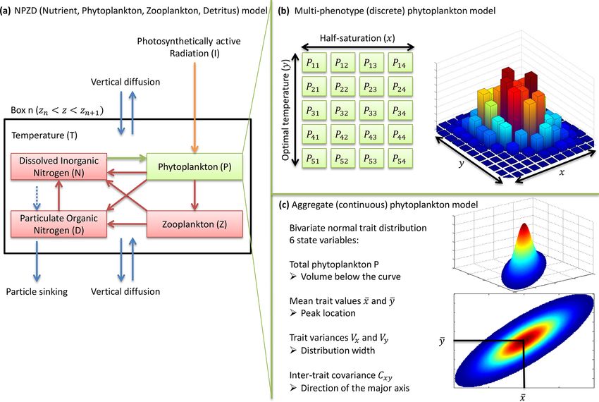
Figure 1. NPZD (nutrient, phytoplankton, zooplankton, detritus) model within its physical setting (a). The phytoplankton pool is represented
by a discrete set of species with different traits (b) or by moments of the trait distributions, assuming a bivariate normal distribution (c).
Colours in (b) and (c) represent phytoplankton concentration.
ent limitation factor γn (N, x). The half-saturation constant a high nitrogen concentration (u∞ −1
p (T , I, x, y); d ) and the
Kn (x) is the DIN concentration at which the nitrogen up- affinity for nitrogen (fp (T , I, x, y); d mmol m3 ). These
−1 −1
take rate is equal to one-half of the maximum uptake rate for two variables fully define the Michaelis–Menten function for
the same temperature and solar irradiance. As the concen- nutrient uptake. The affinity represents the initial slope of
trations are always positive and span several orders of mag- the curve at zero resource concentration, while the maxi-
nitude,
we use a natural logarithmic scale and define x = mum growth rate represents the horizontal asymptote of the
Kn
log K 0 as our first trait axis, with Kn0 = 1 mmol N m−3 curve that is reached at an infinite resource concentration (see
n
as a reference value for Kn . The half-saturation constant Fig. 2 in Vallina et al., 2019). The affinity is closely related
can be linked to the well-known trade-off between the to the growth rate at a low nitrogen concentration, which is
affinity for a nutrient and the maximum uptake rate, also equal to fp (T , I, x, y)N . The maximum growth rate is re-
known as the gleaner–opportunist trade-off (Frederickson lated to the biomass-specific handling rate of nutrient ions at
and Stephanopoulos, 1981). For a given phenotype, γn (N, x) high nitrogen concentrations. The values of u∞ p (T , I, x, y)
follows a Michaelis–Menten function of nutrient concentra- and fp (T , I, x, y) are given by introducing Eq. (12) into
tion. Eq. (11) and taking the limit of high or low concentrations.
0 ∞
N N u∞
p (T , I, x, y) = up γn (x)γT (T , y)γI (I ) (13)
γn (N, x) = γn∞ (x) = γn∞ (x) 0 x (12)
Kn (x) + N Kn e + N u0p γn∞ (x)γT (T , y)γI (I )
fp (T , I, x, y) =
The nutrient limitation factor at a high nitrogen concentra- Kn (x)
tion, γn∞ (x), is set so that each phenotype has an ecolog- u∞
p (T , I, x, y)
ical niche wherein it grows faster than its competitors. To = (14)
Kn (x)
obtain the expression of γn∞ (x), we first introduce two vari-
ables that represent the competitive ability of phytoplankton In order to prevent phenotypes from dominating all nutri-
in two types of environments: the growth rate in the limit of ent niches (i.e. from being Darwinian demons), we assume
Geosci. Model Dev., 14, 1949–1985, 2021 https://doi.org/10.5194/gmd-14-1949-2021G. Le Gland et al.: SPEAD 1.0 1955
Table 2. Parameters of the ecosystem model.
Symbol Description Value Unit
Phytoplankton parameters
T0 Reference temperature 20 ◦C
u0p Phytoplankton maximum uptake rate for x = 0 and y = T0 1.1 d−1
1T Difference between optimal and maximum temperature 5 ◦C
p Phytoplankton exudation fraction going to DIN 1/3 –
ψp Phytoplankton mortality rate at 20 ◦ C 0.05 d−1
ωp Phytoplankton mortality fraction going to DIN 1/4 –
I0 Phytoplankton optimal irradiance 25 W m−2
χ Phytoplankton photoinhibition factor 12 –
αa Temperature dependence factor for autotrophic processes 0.056 ◦ C−1
Speed multiplied by 1.75 (Q10 ) with a temperature increase of 10 ◦ C
νx Half-saturation diffusivity parameter 10−5 –0.1 –
νy Optimal temperature diffusivity parameter 10−4 –1 ◦ C2
Other ecological parameters
g0 Zooplankton maximum grazing rate at 20 ◦ C 1.5 d−1
Kp Half-saturation for grazing 0.4 mmol N m−3
βz Zooplankton assimilation efficiency 0.4 –
z Zooplankton exudation fraction going to DIN 1/3 –
ψz Zooplankton (quadratic) mortality rate at 20 ◦ C 0.25 (mmol N m−3 ) −1 d−1
ωz Zooplankton mortality fraction going to DIN 1/4 –
ψd PON remineralization rate at 20 ◦ C 0.1 d−1
w PON sinking speed 1.2 m d−1
kw PAR vertical attenuation 0.04 m−1
αh Temperature dependence factor for heterotrophic processes 0.092 ◦ C−1
Speed multiplied by 2.5 (Q10 ) with a temperature increase of 10 ◦ C
Numerical parameters
nx Number of half-saturation values (discrete model) 25 –
ny Number of optimal temperature values (discrete model) 25 –
xmin Minimum half-saturation logarithm (discrete model) −2.5 –
xmax Maximum half-saturation logarithm (discrete model) +1.5 –
ymin Minimum optimal temperature (discrete model) 18 ◦C
ymax Maximum optimal temperature (discrete model) 30 ◦C
zmax Maximum model depth 200 m
that the product of maximum growth and affinity fp u∞ p = has been observed in bacteria and phytoplankton (Healey and
2 Hendzel, 1980; Button et al., 2004; Elbing et al., 2004; Cer-
u∞
p (Kn )−1 is constant with (independent of) x (Meyer meño et al., 2011; Vallina et al., 2019), has been used in
et al., 2015). Therefore, u∞
p is proportional to the square root models (Dutkiewicz et al., 2009; Vallina et al., 2014b; Smith
of Kn and to a factor independent of x, yielding the following et al., 2016; Vallina et al., 2017), and is the simplest way
expression for γn∞ (x): to discriminate the bloom-forming opportunist phytoplank-
√ ton (such as diatoms) from the ubiquitous gleaners (such as
γn∞ (x) = ex = ex/2 . (15) Prochlorococcus) without explicitly representing the com-
plex effects of cell size or the way uptake sites are packed
With this “maximum growth rate–nutrient affinity” trade-off, at the cell surface. However, the thermodynamic bases of the
phenotypes that grow faster than their competitors at high trade-off are still unclear (Wirtz, 2002). For any nutrient con-
nutrient concentrations (high u∞ p ), called opportunists, are centration N, we note that the phenotype
disadvantaged at low concentrations (low fp ) by the same corresponding to
the largest growth rates is x = log KN0 . This is why, under
factor, and those which grow comparatively fast at low nutri- n
ent concentrations (high fp ), called gleaners, are at a disad- the assumption of the gleaner–opportunist trade-off defined
vantage under high concentrations (low u∞ above, Kn defines the optimal nutrient concentration of each
p ). This constraint
https://doi.org/10.5194/gmd-14-1949-2021 Geosci. Model Dev., 14, 1949–1985, 20211956 G. Le Gland et al.: SPEAD 1.0
Figure 2. Phytoplankton growth factors γn (nutrient-dependent), γT (temperature-dependent), and γI (PAR-dependent). Panels (a) and (b)
represent the growth factor as a function of nutrient concentration and temperature, respectively, for different phenotypes. Panels (c) and
(d) represent the growth factor as a function of the corresponding trait for different values of the environmental parameter. The maximum
of each curve corresponds to the phenotype most adapted to a given environment. Panels (e) and (f) are normalized versions of (c) and (d),
respectively, so that their maximum is always 1. Panel (g) is the PAR-dependent growth factor, which is common to all phenotypes in this
version of SPEAD.
x phenotype at which they are competitively superior (Val- specific curves of Eppley (1972):
lina et al., 2017). This result, however, is dependent on the
specific model assumption that fp u∞ (T −y) y + 1T − T
p is a constant. γT (T , y) = e 1T eαa (y−T0 ) . (16)
The second phytoplankton trait that is allowed to mutate in 1T
SPEAD is the optimal temperature. Temperature affects mi-
crobes in two ways. One is generic and applies to the whole The temperature tolerance 1T is set to 5 ◦ C. T0 is a refer-
plankton community. An increase in temperature increases ence temperature with no ecological meaning. For a fixed
the speed of both primary production and heterotrophic pro- value of y, γT (T , y) has a maximum at T = y with a value
cesses for thermodynamic reasons. This effect is often as- of eαa (y−T0 ) . At T = y + 1T and warmer, growth is impos-
sumed to be exponential. In our model, the exponential fac- sible. For a given value of the environment temperature T ,
tor for autotrophic primary production is αa = 0.056 ◦ C−1 , the phenotypes with the largest growth rates have an optimal
which corresponds to a Q10 of 1.75, slightly lower than the temperature y around 2 ◦ C larger than T . This apparent mis-
classical value of 1.88 from Eppley (1972) but higher than match, whereby the dominant phenotype at temperature T
the values based on the metabolic theory of ecology for pho- can grow even faster at temperatures a few degrees warmer,
tosynthesis (López-Urrutia et al., 2006). The second effect is both coherent with other models (Beckmann et al., 2019)
of temperature is phenotype-specific. Each phenotype has an and observed in nature (Thomas et al., 2012; Irwin et al.,
optimal temperature for growth, which is the second trait 2012).
axis and is denoted by y. The effect of temperature on a In this study, the PAR limitation factor γI (I ) is the same
given phenotype (x, y) is asymmetric: at temperatures more for all phenotypes. It includes an optimal PAR (Iopt ) of
than 5 ◦ C above y growth ceases, but temperatures below y 25 W m−2 and photoinhibition above this level. Our value for
merely slow growth. We defined our temperature multiplica- Iopt is in the middle of the range considered by Follows et al.
tive growth factor to be as close as possible to the species- (2007), and our expression for γI (I ) is equivalent to theirs.
Geosci. Model Dev., 14, 1949–1985, 2021 https://doi.org/10.5194/gmd-14-1949-2021G. Le Gland et al.: SPEAD 1.0 1957
In the multi-phenotype model, only nx values of x and ny
− ln(1+χ) I I
− ln(1+χ) I values of y are allowed. The phytoplankton community is
γI (I ) = γI0 1 − e opt e χ Iopt
(17) divided into nx × ny phenotypes. The values of both traits
are explicitly bounded by xmin , xmax , ymin , and ymax . Each
χ + 1 − χ1 ln 1
phenotype is separated from its immediate neighbours by a
γI0 = e χ +1
(18)
χ trait interval 1x = xmax −xmin
nx −1 on x or a trait interval 1y =
ymax −ymin
In the above equation, γI0 is a normalization factor (to en- ny −1 on y. Mutation fluxes at the boundaries (i.e. muta-
sure that γI (I ) cannot exceed 1) and χ is an inhibition factor. tions of the phenotypes with the highest or lowest trait values
The higher the inhibition factor, the less photoinhibition there leading out of the domain) are set to zero. In the interior of
is at irradiances larger than Iopt . In this study, we use χ = 12, our trait domain, the concentration of the phenotype with the
which is the average value in Follows et al. (2007) for large j th value of x and the kth value of y, noted Pj k , is controlled
phytoplankton and corresponds well to published photoinhi- by the following equation, where aj,k = uj,k − gj,k − mj,k ,
bition curves (Platt et al., 1980; Whitelam and Codd, 1983; called the net growth rate, is the sum of all growth and death
Walsh et al., 2001). terms affecting phytoplankton concentration.
For comparison with data, two additional variables can
dPj,k νx
be estimated from the model: primary production and =aj,k (N, T , I )Pj,k +
chlorophyll a concentration. Primary production (PP) is ex- dt (1x)2
pressed in milligrams of carbon per cubic metre per day Pj −1,k uj −1,k + Pj +1,k uj +1,k − 2Pj,k uj,k
(mg C m−3 d−1 ). Our model-based estimate is calculated by νy
+ Pj,k−1 uj,k−1 + Pj,k+1 uj,k+1
multiplying the phytoplankton concentration and the uptake (1y)2
rate, normalizing from nitrogen to carbon with the 106 : −2Pj,k uj,k
(19)
16 Redfield molar ratio (Redfield, 1934) and then convert-
ing from the amount of substance to mass using the molar In all our discrete simulations, we impose xmin = −2.5
mass of carbon (12 g mol−1 ). The chlorophyll a concentra- (Kn = 0.082 mmol N m−3 ), xmax = +1.5 (Kn =
tion (Chl; mg Chl m−3 ) is obtained by dividing the phyto- 4.48 mmol N m−3 ), ymin = 18 ◦ C, and ymax = 30 ◦ C.
plankton concentration in mass of carbon by a variable car- All model values of temperature and DIN concentrations
bon to chlorophyll mass ratio (C : Chl). The C : Chl ratio is are within these boundaries. We set nx = 25 and ny = 25 in
estimated as in Vallina et al. (2008) using a function of depth order to ensure that in most cases 1x and 1y are less than
and time developed by Lefèvre et al. (2002), with parame- the standard deviations of x and y, respectively. Thus, the
ter values calibrated with the observations of Goericke and total number of discrete phenotypes (x,y) is 25 × 25 = 625.
Welschmeyer (1998). At the surface, C : Chl is a sinusoidal In the aggregate model, the trait distribution is assumed
function of the day of year, varying between a maximum of to be continuous. In this case, and contrary to the multi-
160 mg C mg Chl−1 at the summer solstice and a minimum phenotype case, the trait axes are formally unbounded, al-
of 80 mg C mg Chl−1 at the winter solstice. From the depth though phenotypes with extreme trait values always have low
at which I (z, t) = 25 W m−2 to the bottom, C : Chl decreases net growth rates, making them extremely rare. The prognos-
linearly with I (z, t) down to a value of 40 mg C mg Chl−1 tic variables are six statistical moments of the trait distribu-
when light is absent. tion: the total phytoplankton concentration P (t), the mean
trait values x(t) and y(t), the trait variances Vx (t) and Vy (t),
2.2 Aggregate and multi-phenotype models and the inter-trait covariance Cxy (t). They are defined as fol-
lows.
Traits x and y have an infinity of possible values. In or- Z Z
der to solve the equations numerically, the problem needs P (t) = p(x, y, t) · dxdy (20)
to be simplified. Two approaches are considered here. In the Z Z
multi-phenotype or discrete model approach (Fig. 1b), the 1
x(t) = x · p(x, y, t) · dxdy (21)
trait space is discretized, and only a finite number of pheno- P (t)
Z Z
types with fixed trait values are simulated. Phenotypes with 1
y(t) = y · p(x, y, t) · dxdy (22)
intermediate trait values are neglected. In the aggregate or P (t)
continuous model approach (Fig. 1c), the state variables are 1
Z Z
total phytoplankton concentration, the mean trait values, the Vx (t) = (x − x(t))2 p(x, y, t) · dxdy (23)
P (t)
trait variances, and the inter-trait covariance. In the continu- Z Z
1
ous trait model, a specific shape of the trait distribution must Vy (t) = (y − y(t))2 p(x, y, t) · dxdy (24)
be assumed a priori (Wirtz and Eckhardt, 1996; Bruggeman P (t)
Z Z
and Kooijman, 2007). In the discrete trait model, the trait dis- 1
Cxy (t) = (x − x(t)) (y − y(t)) p(x, y, t)
tribution is an emergent property, and thus it does not need P (t)
to be assumed beforehand. · dxdy (25)
https://doi.org/10.5194/gmd-14-1949-2021 Geosci. Model Dev., 14, 1949–1985, 20211958 G. Le Gland et al.: SPEAD 1.0
The second-order moments (Vx , Vy and Cxy ) are difficult dVy ∂ 2a ∂ 2a 2
2 ∂ a
= Vy2 2 + 2Vy Cxy + Cxy + 2νy
to interpret directly due to their dimensions. In the analyses, dt ∂y ∂x∂y ∂x 2
we thus transform variances into standard deviations (σx and 1 ∂ 2u 1 ∂ 2u ∂ 2u
σy ) and covariance into correlation (Rxy ) as follows: u(x, y, t) + Vx 2 + Vy 2 + Cxy (33)
2 ∂x 2 ∂y ∂x∂y
p dCxy ∂ 2a 2 ∂ 2a
σx (t) = Vx (t), (26) = Vx Cxy 2 + (Vx Vy + Cxy )
q dt ∂x ∂x∂y
σy (t) = Vy (t), (27) 2
∂ a
+ Vy Cxy 2 (34)
Cxy (t) ∂y
Rxy (t) = . (28)
σx (t)σy (t)
The net growth rate a = u − g − m and its derivatives
These three diagnostic variables, along with P , x, and y, with respect to traits are in all cases taken near the mean
are also computed for the multi-phenotype model for com- trait values (x and y) and for the values of N, T , and I at
parison. The standard deviations have the same dimensions time t. The growth rate of the whole phytoplankton commu-
as the mean traits and can thus be compared to them. Eco- nity depends first on the net growth rate of the most abun-
logically, they represent trait diversity. Inter-trait correla- dant phenotype (the “winner”
of the competition), a(x,y, t),
∂2a ∂2a ∂2a
tion is a dimensionless number between −1 and +1, which with correction terms 2 Vx ∂x 2 + 21 Vy ∂y
1
2 + Cxy ∂x∂y for
is easier to interpret than the covariance. A correlation of the less abundant and generally less fit phenotypes (“losers”).
−1 means above-average values of x always coincide with Mean traits increase when larger trait values are associated
below-average values of y and vice versa. A correlation of ∂a
with larger net growth rates ∂x > 0 or ∂a∂y > 0 and de-
+1 means above-average values of x always coincide with
∂a
above-average values of y. A correlation of 0 means all com- crease in the opposite case ∂x < 0 or ∂a
∂y < 0 . The change
binations are equally possible (i.e. the two traits are indepen-
is faster when trait variances Vx and Vy are high. As a
dent). consequence, the overall effect of trait diversity on pri-
We follow the method developed by Norberg et al. (2001), mary production depends on the environmental conditions.
based on Taylor expansions of the uptake and net growth In a stable environment, high trait variances diminish the
rates to derive the differential equations for the moments of primary production because phenotypes with low growth
the trait distribution. We assume a bivariate normal distri- rates are present. Under frequent disturbances, however,
bution of traits, which is a generalization of the 1D Gaus- high trait variances increase the short-term adaptive capac-
sian function. Normal distributions are observed in nature for ity, allowing the community to maintain mean traits close
the logarithm of size (Cermeño and Figueiras, 2008; Quin- to the optimum and thereby increasing primary produc-
tana et al., 2008; Downing et al., 2014) and are convenient tion (Smith
assumptions for models because they produce the simplest et al., 2016). We note that when traits covary
Cxy 6 = 0 , the change in each trait depends on both nu-
forms for the equations (Wirtz and Eckhardt, 1996; Merico ∂a ∂a
trient concentration N Vx ∂x for x and Cxy ∂x for y and
et al., 2009). The derivation is explained in detail in Ap-
pendix B. In the absence of trait diffusion, our equations are water temperature T Vy ∂a ∂a
∂y for y and Cxy ∂y for x . Vari-
a particular case of the general equations derived by Brugge- ances decrease due to competition when mean trait values
man (2009) for multivariate normal trait distributions. In the are
2 close to the2 values that maximize the net growth rate
single-trait case, they are simpler than the original equations ∂ a ∂ a
< 0 and ∂y 2 < 0 . This is most often the case, since
∂x 2
of Merico et al. (2014) and identical to the more recent for-
phenotypes that are not optimal tend to be outcompeted. Trait
mulation of Coutinho et al. (2016). In the absence of physical
diversity must therefore be maintained by some other pro-
transport, the differential equations followed by the prognos-
cess: this is the role of trait diffusion. In these equations,
tic variables are as follows.
trait diffusion
is a (positive) source of variance equal to
1 ∂2u 1 ∂2u ∂2u
1 ∂ 2a 1 ∂ 2a ∂ 2a
dP 2νx/y u(x, y, t) + 2 Vx ∂x 2 + 2 Vy ∂y 2 + Cxy ∂x∂y but does
= P a(x, y, t) + Vx 2 + Vy 2 + Cxy (29)
dt 2 ∂x 2 ∂y ∂x∂y not affect the equations for phytoplankton concentration,
dx ∂a ∂a mean traits, or covariance. This is coherent with the fact that
= Vx + Cxy (30)
dt ∂x ∂y mutations are symmetrical (no effect on x and y) and neither
dy ∂a ∂a create nor remove biomass (no effect on P ). Trait diffusion
= Vy + Cxy (31) does not affect covariance because mutations of the two traits
dt ∂y ∂x
2
are independent of each other. There is no mechanistic re-
dVx ∂ a ∂ 2a 2
2 ∂ a lationship between optimal temperature and half-saturation.
= Vx2 2 + 2Vx Cxy + Cxy + 2νx
dt ∂x ∂x∂y ∂y 2 Mutations can create all combinations: cold-water gleaners,
1 ∂ 2u 1 ∂ 2u ∂ 2u
warm-water gleaners, cold-water opportunists, and warm-
u(x, y, t) + Vx 2 + Vy 2 + Cxy (32) water opportunists. However, by increasing variances, trait
2 ∂x 2 ∂y ∂x∂y
Geosci. Model Dev., 14, 1949–1985, 2021 https://doi.org/10.5194/gmd-14-1949-2021G. Le Gland et al.: SPEAD 1.0 1959
ues P (Vx + x 2 ), P (Vy + y 2 ), and P (Cxy + x y) . Follow-
diffusion decreases the absolute value of correlation. Only
the environment can correlate the traits by favouring some ing the method of Bruggeman (2009), we therefore use these
combinations over others. Although correlation is defined as conserved moments as tracers involved in physical transport.
a local quantity, for a given depth and time, it is expected Their full Eulerian derivatives are computed as follows using
to be influenced by the spatio-temporal patterns of environ- the product rule.
ment variations because local communities always contain
remnants of past communities and migrants from other loca- ∂ (P x) dx dP ∂ ∂ (P x)
=P +x + κz (39)
tions. ∂t dt dt ∂z ∂z
∂ (P y) dy dP ∂ ∂ (P y)
2.3 Physical setting =P +y + κz (40)
∂t dt dt ∂z ∂z
∂ P Vx + x 2
SPEAD 1.0 has one spatial dimension: the vertical. A depth- dVx dx
=P + 2P x + Vx + x 2
resolved simulation is the minimum physical setting in the ∂t dt dt
!
ocean to resolve the different temperature and nutrient niches dP ∂ ∂ P Vx + x 2
and the decisive effect of the vertical mixing on the variances + κz (41)
dt ∂z ∂z
and the covariance. The model is divided into 20 vertical lev-
∂ P Vy + y 2
els from the surface to 200 m deep, with a uniform vertical dVy dy
step of 10 m. =P + 2P y + Vy + y 2
∂t dt dt
Two processes can transport matter from one vertical level ∂ P Vy + y 2
!
dP ∂
to another and thus need to be added to the differential equa- + κz (42)
tions of the 0D model presented in Sect. 2.1 and 2.2. First, dt ∂z ∂z
PON sinks at a speed of w = 1.2 m d−1 . Sinking is repre-
∂ P Cxy + x y dCxy dx dy
sented by an extra term in the PON equation (Eq. 4) equal to =P +Py +Px
∂t dt dt dt !
−w ∂D∂z , where z is depth and is always positive. The vertical
dP ∂ ∂ P Cxy + x y
derivative ∂D∂z is solved by a first-order upwind scheme. Sec-
+ Cxy + x y + κz (43)
dt ∂z ∂z
ond, tracers are vertically mixed by turbulent diffusion. Ver-
tical turbulent diffusion (called vertical diffusion from now
The above Eulerian derivatives are the derivatives used in
on, which is unrelated to trait diffusion) tends to homogenize
SPEAD to proceed from one time step to the next. Then, at
the spatial distribution of each tracer. It is controlled by the
each time step, we recover
the necessary statistical moments
vertical diffusivity parameter κz , expressed in square metres
x, y, Vx , Vy , and Cxy by back-computing them.
per day (m2 d−1 ). The vertical
diffusion of a conserved tracer
∂ ∂A(z,t)
A is ∂z κz (z, t) ∂z . This expression applies to all con- (P x)
x= (44)
centrations of the discrete model and to concentrations N , P , P
Z, and D of the continuous trait model. As a consequence, (P y)
their full local (Eulerian) time derivatives at a given depth z y= (45)
P
are as follows. P Vx + x 2
(P x)2
Vx = − (46)
P P2
∂Z dZ ∂ ∂Z
= + κz (35) P Vy + y 2
(P y)2
∂t dt ∂z ∂z Vy = − (47)
P 2
P
∂N dN ∂ ∂N
= + κz (36) P Cxy + x y (P x) (P y)
∂t dt ∂z ∂z Cxy = − (48)
∂D dD ∂
∂D
∂D P P P
= + κz −w (37)
∂t dt ∂z ∂z ∂z The derivatives with respect to z used in the vertical diffusion
∂P dP ∂ ∂P terms are estimated by an implicit scheme in order to avoid
= + κz (38) numerical instability. The depth-resolved model is solved in
∂t dt ∂z ∂z
time with a fourth-order Runge–Kutta numerical scheme.
In contrast, the vertical turbulent diffusions of the statisti- Three environmental forcings are necessary to run the
cal moments x, y, Vx , Vy , and Cxy do not follow a simple model: temperature, PAR, and vertical diffusivity. All three
analytical expression because they are not material quanti- depend on depth and time and have been set to values from
ties and thus are not conserved during mixing. For instance, the Sargasso Sea. The forcings are seasonal. Inter-annual
the mixing of two phytoplankton communities with different variations and the day–night cycle are neglected. Temper-
mean traits creates additional trait variance. Fortunately, ver- ature and surface PAR (I0 (t)) directly affect the rates of
tical mixing conserves the sums of phytoplankton trait val- plankton growth and death. They are set for each day using
ues (equal to P x and P y) and the sum of squared trait val- observations collected during the Bermuda Atlantic Time-
https://doi.org/10.5194/gmd-14-1949-2021 Geosci. Model Dev., 14, 1949–1985, 20211960 G. Le Gland et al.: SPEAD 1.0
series Study (BATS) (Steinberg et al., 2001). PAR avail- all simulations. We checked that departing from this ratio
ability is assumed to decrease exponentially with depth did not qualitatively affect our results. In total, we conducted
I (z, t) = I0 (t)e−kw z , with a PAR vertical attenuation co- simulations for 10 sets of mutation rates, including the con-
efficient (kw ) of 0.04 m−1 . Self-shading by phytoplankton trol case.
is neglected. The vertical diffusivity κz is the third forcing. A two-trait model is not simply the superposition of two
Contrary to temperature and PAR, it has not been directly one-trait models for at least two reasons. First, when two
observed. Therefore, the turbulent diffusivity comes from the environmental factors limit biomass growth but only one is
physical model GOTM for the Sargasso Sea (Bruggeman and included in the model, the simulation is likely to overesti-
Bolding, 2014). All three forcings as functions of time and mate the phytoplankton growth rate. Second, when there is
depth are shown in Fig. 3. a strong inter-trait correlation, each environmental factor im-
pacts both traits. For instance, if the ambient DIN concentra-
2.4 List of simulations tion (N) is below the (geometric) mean half-saturation con-
stant (ex ), the competition for nutrients will select for phe-
The simulation of the aggregate two-trait model with muta- notypes with a lower half-saturation constant. If at the same
tion rates νx = 0.001 and νy = 0.01 ◦ C2 is our standard sim- time the half-saturation is negatively correlated with optimal
ulation for this study. νx is expressed without a unit because temperature (i.e. if phenotypes with low half-saturation con-
the trait axis x is in logarithmic scale, but like νy it is a vari- stants also tend to have high optimal temperatures), the com-
ance increase per generation. Most of the results presented petition for nutrients will also increase the concentrations of
in Figs. 4, 5, 6, 7, and 9 come from this standard simulation. phenotypes with high optimal temperatures, in addition to the
The bulk properties of SPEAD 1.0 (total primary production, effect of environment temperature. In the conceptual model
total phytoplankton biomass, nutrient and detritus concentra- of Savage et al. (2007), the inter-trait correlation in a two-trait
tions) are validated using observations from the BATS sta- model led to higher variances and to a considerable improve-
tion in the Sargasso Sea (Steinberg et al., 2001; Vallina et al., ment in the ability of the mean phytoplankton traits to track
2008; Vallina, 2008). The multi-phenotype discrete version optimal values controlled by environmental conditions com-
of SPEAD is used to validate (i) the assumption made in pared with one-trait models. In order to know whether these
the aggregate continuous model that traits are normally dis- results also apply to our model, we compare the dynamics
tributed and (ii) the simulated values and tendencies of the of traits x and y in SPEAD to the dynamics of simplified
moments of the continuous trait distribution. In order to bet- one-trait models wherein either x or y varies between phe-
ter understand the behaviour of the model, the standard sim- notypes and the other trait is optimized instantaneously (i.e.
ulation is also compared to simulations with different muta- set to the optimal value at each location and time given the
tion rates and to simulations with adaptive dynamics for only environmental conditions).
one trait, keeping the other trait unable to mutate but at its The time step for our simulations is 6 h. At the first time
optimal value. step and at all vertical levels, the DIN concentration is ini-
Trait diffusion is a relatively recent concept, and the values tialized to 1.8 mmol N m−3 , phytoplankton and zooplankton
of the mutation rates are not yet well calibrated by observa- concentrations to 0.1 mmol N m−3 , and the PON concentra-
tions. To obtain a qualitative idea of the ecosystem model be- tion to 0.0 mmol N m−3 . The total amount of nitrogen in the
haviour, we tried a wide range of values for νx (from 0.00001 water column is conserved, and every loss below 200 m due
to 0.1). The largest value was chosen for its similarity to the to PON sinking is compensated for by an equivalent gain
trait diffusivity parameter used by Merico et al. (2014) and of DIN, also at 200 m. Mean logarithm of half-saturation
Chen and Smith (2018) to account for the observed trait vari- and mean optimal temperature are initialized at −0.5 (cor-
ance. However, νx = 0.1 allows the phytoplankton to reach a responding to Kn = 0.61 mmol N m−3 ) and 24 ◦ C, respec-
variance of Vx = 4 in only 20 generations, since 2νx is added tively, with initial standard deviations of 0.1 and 0.3 ◦ C. Each
to the phytoplankton population variance at each generation. simulation is run for at least 3 years and until convergence is
This variance is the maximum allowed in the discrete model reached. Our convergence criterion is that, for every day of
and corresponds to having half the community at each ex- year and every depth level, the difference between the last
treme of the trait axis (x = −2.5 and x = +1.5). However, 2 years should be less than 0.1 % for P , Vx , and Vy , less than
laboratory experiments based on single clones show signifi- 0.1 % of the modelled range for x and y, and less than 0.001
cant evolution only on timescales of hundreds to thousands for Rxy . In other words, convergence is achieved when the
of generations (Schlüter et al., 2016). For this reason we seasonal cycle of the model state variables is repeated from
also conducted simulations with mutation rates as low as year to year. The results shown are in all cases from the last
0.00001 and a control simulation without trait diffusion at simulated year. We checked that total nitrogen was the only
all (νx = 0). As the mutation rate has the dimension of trait feature in the initial conditions that affected the results.
squared and as the range of temperature is around 3 times
larger than the range of nutrient concentration logarithms,
ν
we fixed the same ratio of mutation rates, νyx = 10 ◦ C2 , for
Geosci. Model Dev., 14, 1949–1985, 2021 https://doi.org/10.5194/gmd-14-1949-2021You can also read