Freshwater in the Arctic Ocean 2010-2019
←
→
Page content transcription
If your browser does not render page correctly, please read the page content below
Ocean Sci., 17, 1081–1102, 2021
https://doi.org/10.5194/os-17-1081-2021
© Author(s) 2021. This work is distributed under
the Creative Commons Attribution 4.0 License.

Freshwater in the Arctic Ocean 2010–2019
Amy Solomon1,2 , Céline Heuzé3 , Benjamin Rabe4 , Sheldon Bacon5 , Laurent Bertino6 , Patrick Heimbach7 ,
Jun Inoue8 , Doroteaciro Iovino9 , Ruth Mottram10 , Xiangdong Zhang11 , Yevgeny Aksenov5 , Ronan McAdam9 ,
An Nguyen12 , Roshin P. Raj6 , and Han Tang11
1 Cooperative  Institute for Research in Environmental Sciences, University of Colorado Boulder, Boulder, Colorado, USA
2 Physical Sciences Laboratory, NOAA Earth System Research Laboratory, Boulder, Colorado, USA
3 Department of Earth Sciences, University of Gothenburg, Gothenburg, Sweden
4 Climate Sciences Division, Alfred-Wegener-Institut Helmholtz-Zentrum für Polar-

und Meeresforschung, Bremerhaven, Germany
5 Marine Physics and Ocean Climate Division, National Oceanography Centre, Southampton, UK
6 Nansen Environmental and Remote Sensing Center and Bjerknes Center for Climate Research, Bergen, Norway
7 Department of Geological Sciences, Jackson School of Geosciences, University of Texas, Austin, Texas, USA
8 Division for Research and Education, Meteorology and Glaciology Group,

National Institute of Polar Research, Tachikawa, Japan
9 Centro Euro-Mediterraneo per i Cambiamenti Climatici, Bologna, Italy
10 Danish Meteorological Institute, Copenhagen, Denmark
11 Department of Atmospheric Sciences, University of Alaska Fairbanks, Fairbanks, Alaska, USA
12 Oden Institute for Computational Engineering and Sciences, The University of Texas at Austin, Austin, Texas, USA

Correspondence: Amy Solomon (amy.solomon@noaa.gov)

Received: 23 November 2020 – Discussion started: 8 December 2020
Revised: 22 June 2021 – Accepted: 27 June 2021 – Published: 17 August 2021

Abstract. The Arctic climate system is rapidly transitioning       salty Atlantic waters have shoaled. During 2000–2010, the
into a new regime with a reduction in the extent of sea ice,       Arctic Oscillation and moisture transport into the Arctic are
enhanced mixing in the ocean and atmosphere, and thus en-          in-phase and have a positive trend. This cyclonic atmospheric
hanced coupling within the ocean–ice–atmosphere system;            circulation pattern forces reduced freshwater content on the
these physical changes are leading to ecosystem changes in         Atlantic–Eurasian side of the Arctic Ocean and freshwater
the Arctic Ocean. In this review paper, we assess one of the       gains in the Beaufort Gyre. We show that the trend in Arctic
critically important aspects of this new regime, the variability   freshwater content in the 2010s has stabilized relative to the
of Arctic freshwater, which plays a fundamental role in the        2000s, potentially due to an increased compensation between
Arctic climate system by impacting ocean stratification and        a freshening of the Beaufort Gyre and a reduction in fresh-
sea ice formation or melt. Liquid and solid freshwater exports     water in the rest of the Arctic Ocean. However, large inter-
also affect the global climate system, notably by impact-          model spread across the ocean reanalyses and uncertainty in
ing the global ocean overturning circulation. We assess how        the observations used in this study prevent a definitive con-
freshwater budgets have changed relative to the 2000–2010          clusion about the degree of this compensation.
period. We include discussions of processes such as poleward
atmospheric moisture transport, runoff from the Greenland
Ice Sheet and Arctic glaciers, the role of snow on sea ice,
and vertical redistribution. Notably, sea ice cover has become
more seasonal and more mobile; the mass loss of the Green-
land Ice Sheet increased in the 2010s (particularly in the
western, northern, and southern regions) and imported warm,

Published by Copernicus Publications on behalf of the European Geosciences Union.
1082                                                                 A. Solomon et al.: Freshwater in the Arctic Ocean 2010–2019

1     Introduction                                                       seawater, either as a freshwater volume or a freshwater flux
                                                                         component of a seawater volume or flux. It usually manifests
1.1    Freshwater in the Arctic Ocean                                    as a small fraction of the seawater volume or flux, where
                                                                         the fraction takes the form (δS/Sref ) and where δS = −Sref
Rapid changes in the Arctic climate system are impact-                   is the deviation of the seawater salinity S from a reference
ing marine resources and industries, coastal Arctic environ-             value Sref . The sign in the numerator is conventionally re-
ments, and large-scale ocean and atmosphere circulations.                versed so that a positive-scaled salinity anomaly reflects a
The Arctic climate system is rapidly transitioning into a new            freshwater reduction and vice versa. However, scientists’ fa-
regime with a reduction in the extent of sea ice (Stroeve                miliarity with this usage perhaps disguises the fact that it is
and Notz, 2018), a thinning of the ice cover (Kwok, 2018),               an arbitrary construct: the concept of “reference salinity” and
a warming and freshening of the Arctic Ocean (Timmer-                    values attributed to it are not rigorously mathematically and
mans and Marshall, 2020), regionally enhanced mixing in                  physically defined.
the ocean and atmosphere, and enhanced coupling within                      Since this is a review of existing literature and in light of
the ocean–ice–atmosphere system (Polyakov et al., 2020a);                established practice, we continue to employ here the “tradi-
these physical processes are leading to cascading changes in             tional” approach to freshwater flux calculation by use of a
the Arctic Ocean ecosystems (Bluhm et al., 2015; Polyakov                fixed reference salinity. For completeness we include a dis-
et al., 2020a). The emergent properties of this new regime,              cussion of recent studies that highlight the ambiguity that
termed the “New Arctic” (Jeffries et al., 2013), are yet to              arises when a constant reference salinity is used to calculate
be determined since altered feedback processes are expected              freshwater fluxes. The significant freshwater flux differences
to further impact upper ocean heat and freshwater content,               that can arise from the use of different reference salinities are
atmospheric and oceanic stratification, the interactions be-             illustrated and quantified by Tsubouchi et al. (2012) as well
tween subsurface or intermediate warm waters and surface                 as by Schauer and Losch (2019). Schauer and Losch (2019)
cold and fresh layer, among other properties (Carmack et al.,            argue that it is preferable to use the uniquely defined salt bud-
2016). In this review we assess one of the critically important          get as an absolute and well-posed physical quantity. How-
aspects of this new regime, the variability of Arctic freshwa-           ever, Bacon et al. (2015) observed that a true freshwater flux
ter.                                                                     occurs without ambiguity at the surface where freshwater is
   Freshwater in the Arctic Ocean plays a critical role in the           exchanged between ocean and atmosphere (via precipitation
global climate system; by impacting large-scale overturning              and evaporation) and where the ocean receives freshwater in-
ocean circulations (Sévellec et al., 2017; see Fig. 1 showing            put from the land (as river or other runoff). This atmosphere–
basins and upper circulation) by changing ocean stratification           ocean surface freshwater flux is a key element of the global
that affects sea ice growth, biological primary productivity             freshwater cycle, predicted to amplify with global warming,
(Ardyna and Arrigo, 2020; Lewis et al., 2020), and ocean                 hence the importance of knowledge of this surface flux, its
mixing (Aagaard and Carmack, 1989) and by the emergence                  impacts on the ocean, and the ocean’s redistribution (and
of freshwater regimes that couple variability in land, atmo-             storage) of these impacts. Salinity, by comparison, is of indi-
sphere, and ocean systems (e.g., Jeffries et al., 2013; Wood             rect interest for its role in seawater density, buoyancy, etc.
et al., 2013). Arctic Ocean freshwater is a balance between:             Bacon et al. (2015) recognize that a surface flux requires
    – sources (relatively fresh Pacific oceanic inflow, precipi-         definition of a surface area. They then use a time-varying
      tation, river runoff, ice sheet discharge, and sea ice melt)       ice and ocean control volume (or “budget”) approach, com-
      (Aagaard and Woodgate, 2001; Serreze et al., 2006;                 bined with mass and salt conservation, to generate a closed
      Bamber et al., 2012);                                              mathematical expression where the surface freshwater flux
                                                                         is given by the sum of three terms: (i) the divergence of the
    – sinks (relatively saline Atlantic oceanic inflow, sea              (scaled) salt flux around the boundary of the control volume,
      ice growth, evaporation, and liquid and solid trans-               (ii) the change in total (ice and ocean) seawater mass within
      port through oceanic gateways) (Aagaard and Carmack,               the control volume (or change in mass storage), and (iii) the
      1989; Rudels et al., 1994; Serreze et al., 2006; Haine et          (scaled) change in mass of salt within the control volume (the
      al., 2015);                                                        change in salinity storage). The “scaling” term that emerges
                                                                         from the mathematics performs the same function as the tra-
    – redistribution between Arctic basins and vertical mixing
                                                                         ditional reference salinity but in its place is the control vol-
      (e.g., Timmermans et al., 2011; Morison et al., 2012;
                                                                         ume’s ice and ocean boundary mean salinity, which has un-
      Proshutinsky et al., 2015).
                                                                         comfortable implications in that it can vary in time and with
   These processes are not necessarily independent and are               boundary geography. This is a consequence of the nature of
largely driven by atmospheric variability both within the Arc-           the calculation, which quantifies surface freshwater fluxes.
tic and from lower latitudes.                                            Carmack et al. (2016) interpret the Arctic case thus: the sur-
   Oceanographers have long been accustomed to the use of                face freshwater flux is what is needed to dilute all the ocean
“freshwater” as an identifiable and separable component of               inflows to become the outflows, allowing for interior storage

Ocean Sci., 17, 1081–1102, 2021                                                             https://doi.org/10.5194/os-17-1081-2021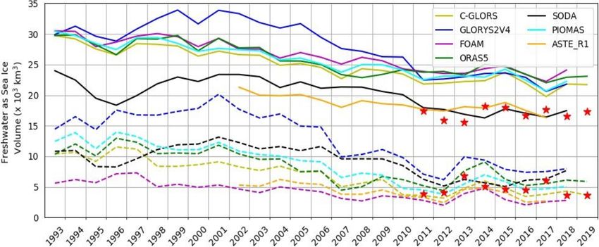
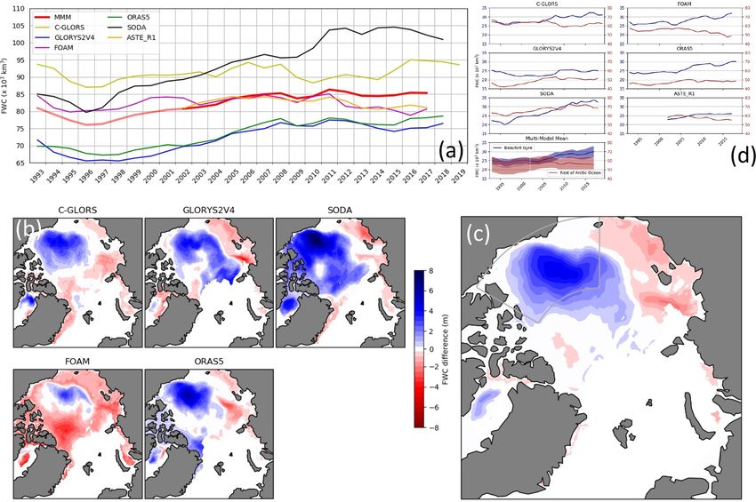
A. Solomon et al.: Freshwater in the Arctic Ocean 2010–2019                                                                1083

changes. An exactly equivalent interpretation is that surface     Labrador Sea and 266 km3 yr−1 from Southeast Greenland
freshwater fluxes and the relatively fresh Bering Strait sea      into the Irminger basin. For comparison, there is a total of
water inflow combine to dilute the relatively saline Atlantic     2440 km3 yr−1 of combined Arctic river runoff over the same
water inflow, which then become the outflows (allowing for        period (Bamber et al., 2012); Haine et al. (2015) provide
storage), where “relatively” means relative to the boundary       numbers of 3900 km3 yr−1 ± 10 % for the 1980–2000 period
mean salinity.                                                    and 4200 km3 yr−1 ± 10 % for the 2000–2010 period, i.e., al-
   Forryan et al. (2019) pursue the surface freshwater flux       most twice as large).
approach, noting that (as is well known, e.g., Östlund and           The upper Arctic Ocean is hence characterized by salin-
Hut, 1984) evaporation and freezing are distillation processes    ity values lower than that of the inflow of waters of largely
that leave behind a geochemical imprint via oxygen isotope        Atlantic origin through the Fram Strait and the Barents Sea
anomalies on the affected freshwater in the sea ice and sea-      opening. The result is an extremely stratified Arctic Ocean
water. In the case of evaporation, distillation (here, isotopic   with a shallow seasonal mixed layer on average less than
fractionation) preferentially removes lighter oxygen isotopes     100 m thick and a halocline that is the result of all the in-
from seawater, leaving behind in the seawater a proportion        flows (McLaughlin et al., 1996; Rudels et al., 2004). Below
of heavier isotopes. The lighter isotopes that are now in the     the halocline sits the “Atlantic layer”, which is comparatively
atmosphere return to the land or sea surface as precipitation.    warm and salty, and below this are the Arctic Ocean deep wa-
Those falling on land can (eventually) transfer from land to      ters (Aagaard et al., 1985; Rudels, 2012). Vertical fluxes of
sea by river runoff, by other glacial processes, or by further    freshwater are generally low due to this strong stratification
cycles of evapotranspiration and precipitation. For sea ice,      and very low vertical turbulent mixing and diffusion (e.g.,
the ice contains the lighter isotopes while heavier isotopes      Fer, 2009). The reviews of Carmack et al. (2016) and Haine
are contained in the brine that drains out of the ice during      et al. (2015) confirm the picture above; hence, they mainly
freezing to re-enter the ocean. The isotopically lighter me-      considered the Arctic freshwater budget in the near-surface
teoric fractions are used to quantify freshwater that origi-      layers. This current study expands on their work and de-
nates from the atmosphere (directly or indirectly), and the       scribes the processes impacting the vertical (re)distribution
isotopically heavier fractions similarly quantify the signal of   of freshwater throughout the entire water column.
brine rejected from sea ice and thereby the amount of ice            Assessments of Arctic freshwater for the 2000–2010 pe-
formed from that seawater. The Forryan et al. (2019) study        riod relative to 1980–2000 were completed as part of the
shows that, within uncertainties, the geochemical approach        WCRP/IASC/AMAP Arctic Freshwater Synthesis (Prowse
produces the same surface freshwater flux as the budget ap-       et al., 2015; Carmack et al., 2016; Vihma et al., 2015) and
proach.                                                           the Arctic–Subarctic Ocean Fluxes program (Haine et al.,
   Freshwater input to the Arctic Ocean is almost entirely        2015). These projects found that liquid freshwater increased
confined to the upper water column and comes in the form          by 25 % (5000 km3 ) in the Beaufort Gyre; the Beaufort High
of continental runoff, including from glacier melt, waters        was stronger than normal with higher sea level, a deeper
of Pacific origin, various coastal currents, and precipita-       halocline, stronger anticyclonic flow, and stronger transpolar
tion. In addition, freshwater input from the Greenland Ice        drift (Proshutinsky et al., 2009; McPhee et al., 2009; Rabe et
Sheet and other marine terminating glaciers has three subsur-     al., 2011; Haine et al., 2015). However, estimates of fluxes
face contributions: (i) melting from calved icebergs (Moon        through the Fram Strait and the Labrador Sea were either too
et al., 2017), (ii) submarine melt rates that may produce a       uncertain or showing statistically insignificant changes, lead-
freshwater plume, which may or may not become neutrally           ing to speculation on whether freshwater accumulated in the
buoyant below the surface (Straneo et al., 2011), and sub-        Arctic Ocean, if released via these Arctic gateways, could
glacial runoff. Melt plumes that are amplified by seasonal        substantially impact the global ocean overturning circulation
subglacial runoff are more likely to reach the surface. Jenk-     and climate (e.g., Haine, 2020; Zhang et al., 2021). In these
ins (2011) refers to a melt plume in the absence of sub-          studies, processes such as the redistribution of freshwater be-
glacial runoff as “melt-driven convection”, whereas runoff        tween basins and vertical redistribution due to turbulent mix-
(an added buoyancy source) incurs “convection-driven melt-        ing were not taken into account, leading to uncertainty in this
ing”. Overall, the freshwater flux magnitude from Greenland       speculation.
into the Arctic Mediterranean remains small compared to              The observed Beaufort Gyre freshening is illustrated in
that of Arctic river runoff for the 1961–1990 period. Bam-        Fig. 2, which shows 1993–2019 annual mean Arctic Ocean
ber et al. (2012) estimate around 184 km3 yr−1 freshwater         freshwater from seven state-of-the-art global ocean reanaly-
flux from North and Northeast Greenland into the Arctic           ses (ORAs; see Table 1 for a description of the models used
Mediterranean. Given that this region is mostly on the con-       in this study). Significant freshening in the Beaufort Gyre is
tinental shelves adjacent to the Fram and Nares straits, it       seen in 2010–2017 means minus 2000–2010 means in six
is likely that much of the discharge from northern Green-         ORAs (Fig. 2b, not including ASTE_R1, using the common
land is rapidly exported. Another 432 km3 yr−1 from West          2010–2017 period for the difference maps). However, this
and Southwest Greenland are discharged into Baffin Bay and        freshening is partly compensated by a reduction in freshwater

https://doi.org/10.5194/os-17-1081-2021                                                      Ocean Sci., 17, 1081–1102, 2021
1084 A. Solomon et al.: Freshwater in the Arctic Ocean 2010–2019
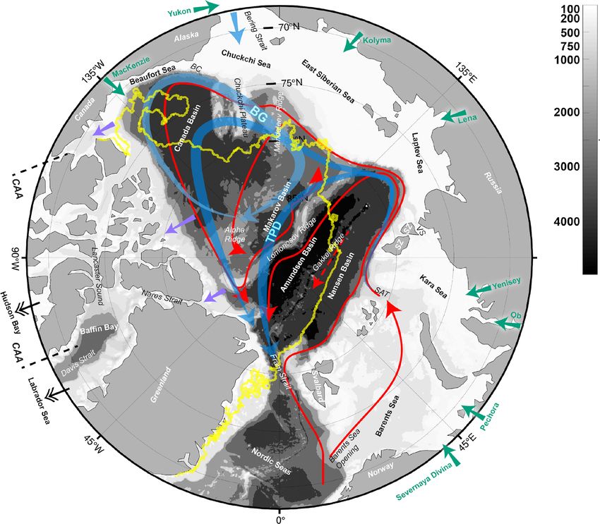
Figure 1. Map of the Arctic Ocean with names of major basins and shelf seas as well as ocean circulation features: major river and Pacific
inflow (cyan and turquoise) and surface outflows (purple), 2020 minimum sea ice edge (yellow), cold and fresh upper ocean circulations
(polar surface water and halocline; blues), and warm and salty Atlantic water circulation (red). Areas shallower than 1000 m are referred
to as shelf areas in the text. BG: Beaufort Gyre; TPD: transpolar drift; BC: Barrow Canyon; CAA: Canadian archipelago; SAT: St. Anna
Trough; VS: Vilkitsky Strait; SZ: Severnaya Zemlya.
in the rest of the Arctic Ocean (Fig. 2b, c). This compensa- In this review we assess to what extent the 2010–2019
tion increases in 2010–2018 compared to 2000–2010, which freshwater budget has changed relative to the 2000–2010 pe-
flattens the total Arctic Ocean freshwater trend when ex- riod. This study is not meant to be a comprehensive assess-
tended to 2019 (Fig. 2a). This is characteristic of the cyclonic ment of all processes that contribute to Arctic freshwater. In-
mode of circulation (Morison et al., 2012, 2021; Sokolov, stead, we focus on specific aspects that provide insight into
1962). However, there is a significant spread in estimates of how the variability has changed since 2010 and the role of
freshwater content in the Beaufort Gyre and the rest of the processes not considered in previous assessments.
Arctic Ocean (Fig. 2d), which prevents a definitive estimate
of the degree of this compensation. The wide variability in 1.2 Arctic freshwater estimates from in situ and
Freshwater Content (FWC) change among the ORAs in the satellite measurements
Siberian Shelf seas is likely due to the paucity of observa-
tions there in recent years. Morison et al. (2021) speculate 1.2.1 Satellite measurements
that the in situ observations have had an increasing spatial
A major challenge in the retrieval of freshwater fluxes in
bias toward the Beaufort Sea. This highlights the need to be
the Arctic Ocean is associated with the lack of availabil-
able to estimate the redistribution of freshwater when assess-
ity of in situ observations. Direct measurements are non-
ing changes in Arctic Ocean freshwater as well as the re-
homogenous in both time and space and rely on spatial as
cent reduction in total Arctic Ocean freshening relative to
well as temporal interpolation, resulting in large uncertain-
the 2000–2010 period.
ties. The ability to estimate freshwater content of the Arctic
Ocean Sci., 17, 1081–1102, 2021 https://doi.org/10.5194/os-17-1081-2021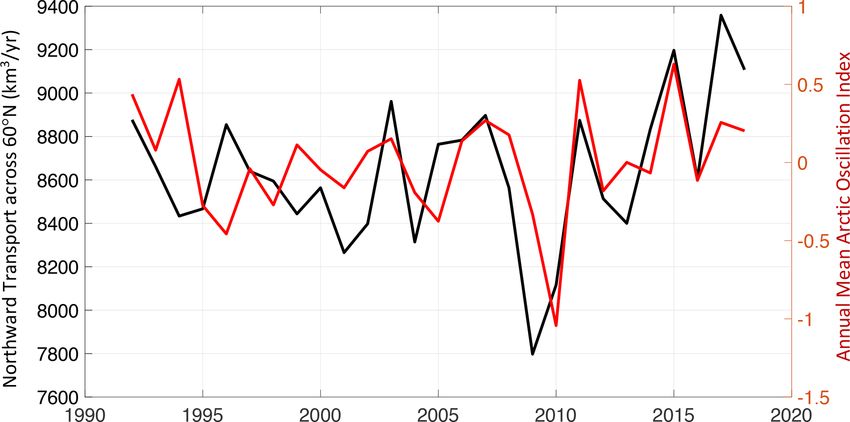
Table 1. Global ocean reanalyses used in this study. T : temperature data; S: salinity; SST: sea surface temperature; SSS: sea surface salinity; SSH: sea surface height; SIC: sea ice
concentration; SIT: sea ice thickness; DA: data assimilation; CORE: Coordinated Ocean-ice Reference Experiment; COARE4: Coupled Ocean–Atmosphere Response Experiment bulk
flux parameterization version 4.
Name C-GLORSv7 FOAM GLORYS2V4 ORAS5 ASRE_R1 SODA3.3.2
Institution CMCC UK MetOffice CMEMS ECMWF Univ. Texas Univ. Maryland
https://doi.org/10.5194/os-17-1081-2021
Austin
Horizontal resolution 0.25◦ 0.25◦ 0.25◦ 0.25◦ 0.3◦ 0.25◦
Vertical resolution 75 z-levels 75 z-levels 75 z-levels 50 z-levels 50 z-levels 50 z-levels
Surface fluxes CORE CORE CORE CORE + wave forcing CORE COARE4
Atmospheric forcing ERA-Interim ERA-Interim ERA-Interim ERA-Interim until Adjusted MERRA2
2014 ECMWF NWP JRA55
A. Solomon et al.: Freshwater in the Arctic Ocean 2010–2019
after 2014
Ocean–sea ice model NEMO3.2- NEMO3.2- NEMO3.1- NEMO3.2- MITgcm MOM5-SIS1
LIM2 CICE LIM2 LIM2
DA variables SIC, Arctic SIT, T , SIC, T , S, SST, SSH SIC, T , S, SST, SIC, T , S, SST, SSH SIC, T , S, SST, T , S, SST, Greenland
S, SSH, SST SSH, runoff SSH and river runoff
DA sources OIv2d, PIOMAS, OSISAFv2, EN4, CERSAT, CMEMS, OSTIA, Olv2d, EN4, ARGO, ITP, WOD, ICOADS,
EN4, AVISO ICOADS, AVHRR AVISO ICES, XBT, AVHRR, Metosat,
AVHRR, ATSR, CTD SEVIRI
AMSRE, AVISOv3
References Storto and Blockley et al. (2014) Garric et al. (2017) Zuo et al. (2019) Nguyen et Carton et al. (2018)
Masina (2016) al. (2021)
Ocean Sci., 17, 1081–1102, 2021
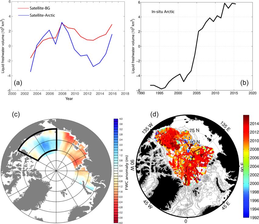
10851086 A. Solomon et al.: Freshwater in the Arctic Ocean 2010–2019 Figure 2. Ordered counterclockwise: (a) Time series of annual freshwater content integrated from 70–90◦ N and down to the 34 isohaline for the 1993–2019 period from six ORAs (in 103 km3 ). Multi-model mean shown in red; darker red indicates all six ORAs are included. (b) Difference (in m) between 2010–2017 and 2000–2010 means in five ORAs (not including ASTE_R1). (c) Multi-model mean of differ- ences (in m) shown in (b). (d) Annual freshwater content separated into contributions from the Beaufort Gyre (blue) and the rest of the Arctic Ocean (red). The lower right figure shows the multi-model mean with ± 1 standard deviation shown with shading. The Beaufort Gyre is defined as 70–80◦ N, 120–180◦ W to be consistent with the satellite estimates below. region indirectly from satellite observations is a major break- equals 34.7 and upper layer salinity equals 27.7. While this through. The methodology, which exploits the satellite de- is a very simple model, the observed signals are significantly rived ocean mass change and satellite altimeter data, is de- larger than the uncertainty, as shown in their thorough uncer- tailed in Giles et al. (2012), Morison et al. (2012), and Ar- tainty assessment (Supplement in Giles et al., 2012). mitage et al. (2016). It derives from the perceptions (1) that Our understanding of the Earth’s gravity field has im- the sea surface height change (as observed by satellite altime- proved considerably over the last decade, thanks to the Grav- ters) is the sum of two components: mass addition (or loss) ity Recovery and Climate Experiment (GRACE) mission and steric expansion (or contraction), and (2) that observa- launched in 2002. GRACE is the only satellite mission de- tion of mass changes (by satellite gravimetry) enables separa- signed to be directly sensitive to mass changes by means tion of these two components. A two-layer model is assumed of gravity. The variability in spatiotemporal characteristics where the sea surface height and interface depth are variable of the Earth’s gravitational field resulting in very small de- and where the upper layer represents the halocline (and sur- viations in the separation between the two satellites of the face mixed layer) and the lower layer all underlying waters. GRACE mission are measured with micrometer precision Upper layer thickness changes (per unit water column area) and are used to infer the Earth’s gravity field, which can then are then a function of changes in sea surface height and water be used to estimate changes in ocean mass (Peralta-Ferriz column mass with assumed layer densities; changes in fresh- et al., 2014; Armitage et al., 2016). Here we use the latest water content are then the thickness changes scaled by S/Sref Release 06 gridded GRACE ocean mass products from the with reversed sign. Giles et al. (2012) assume Sref (their S2 ) Jet Propulsion Laboratory (Watkins et al., 2015). Satellite Ocean Sci., 17, 1081–1102, 2021 https://doi.org/10.5194/os-17-1081-2021
A. Solomon et al.: Freshwater in the Arctic Ocean 2010–2019                                                                     1087

radar altimeters on the other hand can retrieve sea surface          2018). Figure 3a (red line) shows that freshwater content in-
heights in the open ocean with variable precision depending          creases in the Beaufort Gyre during the 2002–2010 period,
on the number of flying altimeters and have been uninter-            followed by a stabilizing phase where the increase flattens
rupted since 1993. CryoSat-2, launched in 2010, is a satel-          out. However, including freshwater content outside of the
lite altimeter that provides coverage up to 88◦ N with much          Beaufort Gyre (blue line in Fig. 3a; defined as the region con-
better spatial resolution than before. Several studies have uti-     toured in Fig. 3c) results in a reduction in freshwater content
lized this source to study the sea level variability of the Arctic   during the 2010–2016 period, indicating increased compen-
(Kwok and Morison, 2016, 2017; Armitage et al., 2018a, b;            sation between freshwater content in the Beaufort Gyre and
Rose et al., 2019; Raj et al., 2020). However, constructing          outside the Beaufort Gyre after 2009. Raj et al. (2020) noted
precise altimeter derived sea level data in the Arctic Ocean         a similar signature in the altimeter derived sea surface height
is still a challenge. One of them is the effect of melt ponds        anomaly and the halosteric component of the sea surface
during summer on the waveforms, which dominate the re-               height anomaly and attributed it to the change in the dom-
flected signal. A better understanding of the radar altime-          inant atmospheric forcing over the Arctic, which changed
ter response over the different ice types must be gained to          from the Arctic dipole pattern to the Arctic Oscillation, re-
improve the quantity and quality of the range retrievals in          spectively, during the time periods prior to and after 2010.
the Arctic Ocean. One of the ongoing efforts is the CRYO-            These results are qualitatively consistent with estimates in
TEMPO project, funded by the European Space Agency.                  Fig. 2 using the ocean reanalyses. In addition, Fig. 2c shows
   Satellites can monitor some important pieces of the Arc-          that the regions not included in Fig. 3 make only small con-
tic freshwater puzzle. Here, we use the state-of-the-art sea         tributions to the time series in Fig. 2. It is well known that
level product produced as part of the recently concluded cli-        while the sea surface height variability in the Beaufort Gyre
mate change initiative (CCI) project (sea level budget clo-          region is dictated by the variability in salinity, the same vari-
sure; Horwath et al., 2020) of the European Space Agency.            ability in the Nordic Seas and the Barents Sea is controlled
This Arctic sea level product (DTU/TUM SLA record; Rose              by Atlantic water temperature as opposed to salinity (Raj et
et al., 2019) is the first one that includes a physical retracker    al., 2020). Hence, the methodology to estimate FWC from
(ALES+) for retrieving the specular waveforms from open              sea surface height data is not recommended in those two re-
leads in the sea cover. The sea state bias corrected using           gions. Our study included the rest of the Arctic excluding the
ALES+ improves the sea level estimates of the region (Pas-           Canadian Archipelago, Nordic Seas, and Barents Sea.
saro et al., 2018). The latest version (v3.1) of the DTU/TUM
SLA record is a complete reprocessing of the former DTU              1.2.2   In situ measurements
Arctic sea level product (Andersen et al., 2016) by dedicated
Arctic retracking. The current study thus takes advantage of         Figure 3b includes estimates of Arctic freshwater content
the state-of-the-art satellite datasets to study the freshwater      from in situ hydrographic observations (black line). The time
content of the region following Giles et al. (2012) and Ar-          series of freshwater content for the whole basin to the 34
mitage et al. (2016).                                                isohaline is extended from Rabe et al. (2014a). Details of
   Freshwater is calculated using the satellite measurements         the mapping procedure and the distribution of hydrographic
using these equations:                                               stations until 2012 are given in Rabe et al. (2014a). Further
                                                                     data are based on the data sources listed in Table 2. Interest-
             S2 − S1      XN
                                                                     ingly, the Arctic satellite and in situ time series in Fig. 3a,
1FWC =                A1 i=0 hi ,                              (1)
                S2                                                   b are relatively consistent before 2009 but do not show the

                    ρ1              m                                same variability after 2009. This difference may stem from
1h = η 1 +                  −1           ,                     (2)
                 ρ2 − ρ1         ρ2 − ρ1                             the lack of data coverage in the in situ measurements, the dif-
where η is the change in SSH, 1m is the ocean mass                   ferent regions used in the time series, and the choice of time
anomaly, N is the number of grid cells, and A is the grid            period for the mean used to obtain anomalies. The satellite
cell area. The salinities S1 and S2 are, respectively, 27.7 and      time series uses the region contoured in Fig. 3c and the in situ
35, while the densities ρ1 and ρ2 are 1022 and 1028, respec-         time series uses observations within the basin excluding the
tively, in units of kg m−3 .                                         shelves, indicating a good part of the difference after 2009
   Time series from 2002 to 2018 using GRACE-derived                 may be due to the contribution by the rest of the basin out-
ocean bottom pressure (OBP) anomalies (https://podaac.jpl.           side the Beaufort Gyre. In addition, the annual values of the
nasa.gov/GRACE, last access: 22 June 2020) and satellite al-         in situ time series are biased towards the prior three years
timeter data provide insights into the redistribution of fresh-      near the end of the time series, as the mapping analysis only
water in the Arctic Ocean (Fig. 3). While initial results from       includes data up to 2015; 2012, 2013 and 2014 show simi-
GRACE suggest an overall OBP decrease caused by a fresher            lar levels as 2015. The locations of all profiles used between
Arctic surface (Morison et al., 2007), results on the now-           1992 and 2015 show that there are interannual variations in
longer time series show more complex interannual variabil-           data coverage but that overall, the decadal timescale is rea-
ity, in agreement with modeling data (e.g., de Boer et al.,          sonably well covered across the Arctic Ocean basin (Fig. 3).

https://doi.org/10.5194/os-17-1081-2021                                                          Ocean Sci., 17, 1081–1102, 2021
1088 A. Solomon et al.: Freshwater in the Arctic Ocean 2010–2019
Figure 3. Anomalies of freshwater content from satellite sea surface height data analysis and GRACE OBP data and from objectively
mapped in situ hydrographic observations. Annual mean time series of freshwater content from (a) satellite measurements in the Beaufort
Gyre (red), the Arctic region shown in (c) (blue), and the (b) Arctic basin using in situ hydrographic observations shown in (d) (black)
in units of 103 km3 . (c) Difference between 2010–2017 and 2002–2010 freshwater content means from satellite measurements in units of
meters. (d) Locations of salinity profiles used for the objective analysis of the in situ data with time denoted by color. Anomalies in (a) and
(b) are relative to the corresponding mean of the 2003–2006 period in each time series using a reference practical salinity of 35 and a layer
from the surface to the 34 isohaline. The Beaufort Gyre region (marked with thick black lines in c) is defined as 70–80◦ N, 120–180◦ W. The
time series are calculated using observations from the Arctic Ocean with a water depth deeper than 500 m and a cutoff at 82◦ N north of the
Fram Strait for the in situ estimates and the contoured region shown in (c) for the satellite estimates. Panel (b) is an update of the time series
in Rabe et al. (2014a), partly shown previously in Wang et al. (2019); the additional data used are listed in Table 2.
2 Changes in Arctic freshwater sources and sinks of freshwater versus salt transports and reference salinities is
provided in Bacon et al. (2015), Schauer and Losch (2019),
The most recent estimates of Arctic freshwater sources and and Tsubouchi et al. (2018). Another more recent devel-
sinks have been developed by Østerhus et al. (2019), Haine opment over the last decade is the inclusion of freshwater
et al. (2015), Prowse et al. (2015), Carmack et al. (2016), fluxes from the Greenland Ice Sheet (GIS) and smaller Arc-
and Vihma et al. (2016). Only Østerhus et al. (2019) covers tic glaciers and ice caps (GICs) into these basins (Bamber et
a more recent period through 2015. One issue is that not all al., 2012, 2018; Dukhovskoy et al., 2019).
these estimates use the same reference salinity; a discussion
Ocean Sci., 17, 1081–1102, 2021 https://doi.org/10.5194/os-17-1081-2021A. Solomon et al.: Freshwater in the Arctic Ocean 2010–2019 1089
Table 2. Sources of salinity data used in the objective analysis to derive the black curve in Fig. 3. The listed data sources are for the data used
in addition to the data described in Rabe et al. (2014a) and published in Rabe et al. (2014b). ITP: ice-tethered profiler; NPEO: North Pole
Environmental Observatory; WHOI: Woods Hole Oceanographic Institution; NABOS: Nansen and Amundsen Basin Observational System.
Expedition, project Year(s) Platform Source URL or contact
Beaufort Gyre Project 2012–2013 Various ships http://www.whoi.edu/beaufortgyre/ (last access: 1 May 2014)
NPEO 2012–2014 Airborne and ice-based ftp://psc.apl.washington.edu/ (last access: 1 May 2014)
WHOI 2012–2015 ITP https://doi.org/10.1029/2009JC005660 (Toole et al., 2016)
PS86 2014 RV Polarstern https://doi.org/10.1594/PANGAEA.853768 (Vogt et al., 2015)
PS87 2014 RV Polarstern https://doi.org/10.1594/PANGAEA.853770 (Roloff et al., 2015)
PS94 2015 RV Polarstern https://doi.org/10.1594/PANGAEA.859558 (Rabe et al., 2016)
NABOS 2013 NABOS https://uaf-iarc.org/nabos/ (last access: 1 May 2014, Polyakov et al., 2003)
2.1 River discharge 2.2 Precipitation and atmospheric moisture transport
Observations suggest a linkage between the Arctic Oscil-
lation (AO) and the North American (mainly Mackenzie Precipitation over the Arctic is the main source of fresh-
River) runoff pathways (Yamamoto-Kawai et al., 2009; Fi- water into the Arctic Ocean, when including that from its
chot et al., 2013). There has been a shift from a rather di- pathway through river discharge from the large continental
rect outflow via the Canadian Arctic Archipelago (CAA) in drainage basins (Haine et al., 2015; Serreze et al., 2006).
the early 2000s to a northward pathway into the Beaufort In climatology, river discharge is predominantly from pre-
Gyre around 2006, coinciding with a change to a strongly cipitation, though land surface processes (e.g., thawing per-
positive AO. In addition, for high AO indices, river runoff mafrost and decreasing vegetation transpiration) may have
entering the Eurasian shelves is mainly transported into the slight contributions according to Zhang et al. (2013). The to-
Canada Basin, while for low AO indices, the transport is tal continental runoff into the Arctic Ocean is about 0.1 Sv
mainly towards the Fram Strait by a strengthened transpolar (see Table 1; Haine et al., 2015). The remaining sources are
drift (Morison et al., 2012; Alkire et al., 2015). lower; those of similar order of magnitude are precipitation–
Observations of runoff rates for Eurasian rivers are avail- evaporation and Bering Strait liquid inflow. In addition, pre-
able since 1936 and for North American rivers since 1964 cipitation is largely driven by atmospheric moisture trans-
(Shiklomanov et al., 2021). There has been a decline since port. Based on a mass-corrected atmospheric moisture trans-
about 1990 in the total gauged area by ∼ 10 % in Siberia port dataset, Zhang et al. (2013) found that the observed in-
and Canada (Shiklomanov et al., 2021), due to the clo- crease in the Eurasian Arctic river discharge was driven by
sure or mothballing of gauging stations. Regardless, only an enhanced poleward atmospheric moisture transport into
the most important rivers are gauged: knowledge of net the river basins. Using the same dataset, Villamil-Otero et
(continent-scale) river discharge rates requires estimation of al. (2017) also found a continual enhancement of the pole-
the substantial ungauged runoff fraction, typically one-third ward atmospheric moisture transport across 60◦ N into the
of the total. The long-term, multi-decadal, gauged annual Arctic Ocean from the 1950s to the mid 2010s. An update
mean runoff rates are given by Shiklomanov et al. (2021) of the transport using ERA5 reanalysis shows a continua-
as 1800 km3 yr−1 (Eurasia, 1936–2015) and 1150 km3 yr−1 tion of the enhancement across 60◦ N (Fig. 4). Nygard et
(North America, 1964–2015), for a total of 2950 km3 yr−1 . al. (2020) also found an increase in poleward moisture trans-
Shiklomanov et al. (2021) also note the increase (with un- port from 1979–2018 using the ERA5 data. Interestingly,
certainties) in these records as 2.9 ± 0.4 (Eurasia, using the they also found that evaporation shows a negative trend due
1935–2015 period) and 0.7 ± 0.3 (North America, using the to suppression by the horizontal moisture transport.
1964–2015 period) km3 yr−2 . The significant Eurasian trend The large-scale atmospheric circulation may play a dy-
is on the order of 15 % per century. However, the weakly namic driving role in the enhanced atmospheric moisture
significant North American trend over the shorter period dis- transport. A statistical analysis indicates a temporally vary-
guises an apparent signal of multi-decadal variability similar ing relationship between the annual moisture transport and
to that observed by Florindo-Lopez et al. (2020), who sug- the annual mean Arctic Oscillation (AO; Thompson and Wal-
gest it to be part of the evidence for much wider-area atmo- lace, 1998), showing a negative and a positive correlation be-
spheric and oceanic teleconnections. fore and after 2000. The positive phase of the AO indicates
a strengthening of the westerlies, transporting atmospheric
moisture to the Eurasian continent and leading to an increase
in precipitation over the landmass (e.g., Kryzhov and Gore-
lits, 2015). An AO positive trend occurred primarily from
the late 1980s to mid-1990s. In the 1990s, the variability of
https://doi.org/10.5194/os-17-1081-2021 Ocean Sci., 17, 1081–1102, 20211090 A. Solomon et al.: Freshwater in the Arctic Ocean 2010–2019
the atmospheric circulation was mainly characterized by the
AO. However, although a positive correlation occurred be-
tween the transport and AO after 2000, the AO lagged the
transport variability by one year during the negative peaks in
2005 and 2010. During 2000–2010, the AO mainly showed
fluctuations and was also inclined towards a negative phase
(Fig. 4). After 2010, the AO and transport are in-phase, with
a positive trend and peak positive values in 2011 and 2015.
During the 2000–2010 time period, the atmospheric circu-
lation spatial pattern experienced a radical change, in par-
ticular during the winter seasons, as revealed in Zhang et
al. (2008). This changed spatial pattern, named the Arctic Figure 4. Time series of annual poleward atmospheric moisture
rapid change pattern (ARP), exhibits a predominant role in transport (in km3 yr−1 ) across 60◦ N updated using the ERA5 re-
driving the poleward moisture transport (Zhang et al., 2013). analysis dataset following Zhang et al. (2013) and the annual mean
This driving role can also be manifested by a poleward ex- Arctic Oscillation (AO) index constructed by NOAA Climate Pre-
tension and intensification of the Icelandic low in the nega- diction Center from 1991–2019. The transport was integrated from
the surface to the top of the atmosphere and along 60◦ N.
tive ARP phase. Considering that temporal-varying features
of AO and the seasonal preference of the emergence of the
spatially transformed ARP, the dynamic driving role of the
atmospheric circulation needs to be further investigated. In which was most pronounced until 2010; their monthly trend
addition, synoptic-scale analysis also suggested the propa- ranges between −537 km3 yr−1 in May and −251 km3 yr−1
gation of intense storms into the Arctic played an important in September. The decrease in sea ice thickness is respon-
role in the enhanced poleward moisture transport and result- sible for 80 % of this trend in winter and 50 % in summer.
ing increase in precipitation (e.g., Villamil-Otero et al., 2017; In addition to the global warming effects, sea ice decrease
Webster et al., 2019). can be attributed to increased downward radiative forcing
Much of the precipitation in the Arctic falls as snow but and turbulent heat fluxes associated with changes in the at-
projections show an increasing amount of rain as the cli- mospheric circulation. In particular, storm activities have in-
mate warms (Bintanja, 2018). This appears to have been ten- tensified over the Arctic Ocean. Recent observational stud-
tatively observed in Greenland, though mostly in southern ies have indicated that storms can increase mixing between
and western Greenland away from the central Arctic Ocean surface cold water and underlying warm water to suppress
(Doyle et al., 2015; Haine et al., 2015; Boisvert et al., 2018; winter sea ice growth or increase summer sea ice melt (Gra-
Oltmanns et al., 2019), where the consequences of surface ham et al., 2019; Peng et al., 2021). Further, even in the
melt, surface runoff, and ice dynamics from increased rain- deep basin area where the Pacific and Atlantic waters lay-
fall over the ice sheet have been observed (e.g., Lenaerts et ers are deeper and stratification is strong, intense storms can
al., 2019). Similarly, Webster et al. (2019) note an increased force Ekman upwelling to cause the intrusions of the deeper
frequency of rain on sea ice. Unfortunately, precipitation warmer and saltier waters in the upper mixed layer. The input
is notoriously difficult to measure, particularly in the solid of deep warm and salty waters and enhanced mixing in the
phase and, as with other observations in the Arctic, reliable mixed layer increase the oceanic heat flux and consequently
observations of precipitation are few and far between. Esti- accelerates summer sea ice melt (Graham et al. 2019; Peng
mates of the precipitation flux are therefore forced to rely et al., 2021; Polyakov et al., 2020a). These processes influ-
on model reanalysis, which have large uncertainties (e.g., ence both the volume of solid freshwater stored in sea ice and
Bromwich et al., 2018) on indirect measures such as river ocean freshwater budgets.
runoff and may also be affected by glacier melt or on GNSS New sea ice in the Arctic forms predominantly over
data analysis of solid earth movements in response to local- the continental shelf. Estimates based on satellite imagery
ized precipitation (e.g., Bevis et al., 2019). puts the cumulative sea ice formation of all Arctic coastal
polynyas to 3000 km3 yr−1 (Tamura and Oshima, 2011), i.e.,
2.3 Sea ice about a quarter of the total mean Arctic sea ice volume.
Consequently, although the shelves receive large amounts of
Freshwater stored in sea ice, i.e., sea ice volume, decreased freshwater from rivers, their largest contribution to freshwa-
by roughly 10 % for maximum sea ice and 40 % for min- ter exchanges comes from sea ice export (e.g., Volkov et al.,
imum sea ice over 2000–2010 (Fig. 5). Kwok (2018) ex- 2020), as the sea ice that forms on the shelves does not stay
plained the flattening by the predominance of seasonal ice. there. Sea ice is instead slowly transported across the Arc-
Using a different approach, Liu et al. (2020) converted sea ice tic by the transpolar drift (Serreze et al., 1989), taking 1.5
age into volume and also found a decrease in sea ice volume to 3 years to travel from the Laptev Sea to Fram Strait (Pfir-
over the entire Arctic of −411 km3 yr−1 over 1984–2018, man et al., 1997; Steele et al., 2004). The transpolar drift
Ocean Sci., 17, 1081–1102, 2021 https://doi.org/10.5194/os-17-1081-2021A. Solomon et al.: Freshwater in the Arctic Ocean 2010–2019 1091
Figure 5. Time series of annual freshwater volume stored as sea ice from seven ORAs and CryoSat-2 (red stars) (in 103 km3 ). The sea ice
volume is calculated as the product of sea ice area and thickness. Annual volume maxima are shown by bold lines, while annual minima are
shown by dashed lines.
and ice deformation rates have been observed to be accel- atmospheric circulations (e.g., Kodaira et al., 2020), would
erating since the early 2000s (Rampal et al., 2011; Spreen cause a delay of snow accumulation on sea ice, the increase
et al., 2011); just recently, the MOSAiC drift expedition has in precipitation and snow depth associated with the increase
shown that the transpolar drift can, indeed, be unusually fast in storm activities in the Pacific Arctic contributes to a rapid
and thus is capable of rapidly transporting sea ice out of the buildup of snow cover on first-year ice (and a potential de-
Arctic (Krumpen et al., 2020). lay in seasonal sea ice melt). These feedbacks were reported
Fram Strait sea ice export is the largest dynamic sink of the by Sato and Inoue (2018) based on the analysis of ice mass
Arctic freshwater cycle. The increase in Fram Strait sea ice balance buoys and CFSR reanalysis datasets. In the Atlantic
export detected from long-term monitoring of sea ice area sector, precipitation associated with six major storm events
has been suspected as the cause of Arctic sea ice volume in 2014–2015 during the N-ICE2015 field campaign (Merk-
loss, in particular for the multiyear thick sea ice within the ouriadi et al., 2017) caused the snow depth to be substantially
Arctic Ocean (Smedsrud et al., 2017; Ricker et al., 2018). greater than climatology.
Using the more recent sea ice thickness retrievals, Spreen et
al. (2020) actually showed that in volume, the Fram Strait 2.4 Freshwater flux from glaciers and the Greenland
export has in fact been decreasing at 27 % per decade over Ice Sheet
1992–2014, on par with the Fram Strait and Arctic ice thick-
ness. In addition to the changes caused by thinned sea ice, The freshwater input from Arctic glaciers and the Greenland
changes in the atmospheric circulation pattern have also sig- Ice Sheet comprises a minor but difficult to compute source
nificantly contributed to the decrease in Fram Strait sea ice of freshwater in the Arctic Ocean basin. The Greenland Ice
export since the mid 1990s (Wei et al., 2019). Sea ice export Sheet and the surrounding smaller peripheral glaciers and
from the Siberian Shelf has increased by 46 % over 2000– ice caps on Greenland have shown an increasing tendency
2014 compared to 1988–1999 and North American sea ice for net ice sheet loss since the early 2000s (Shepherd et al.,
reaches Eurasian waters 37% faster (Newton et al., 2017). 2020; Noël et al., 2017; Bolch et al., 2013), though with wide
But the summer survival rate of sea ice on the Siberian Shelf spatial and large temporal variability from year to year, a
is decreasing by 15 % per decade (Krumpen et al., 2019). trend reflected in other glaciated basins within the Arctic in-
That is, in the 1990s, 50 % of first-year ice entered the trans- cluding Arctic Canada, Russia, and Svalbard (e.g., Noël et
polar drift; now, it is less than 20 %, as the rest melts before al., 2018; Gardner et al., 2011; Moholdt et al., 2012). The
reaching the transpolar drift (Spall, 2019; Krumpen et al., Ice sheet Mass Balance Intercomparison Exercise (IMBIE)
2019). (Shepherd et al., 2012) and IMBIE2 (Shepherd et al., 2020)
Snow on sea ice is crucial for surface heat budgets through results show, for example, a steady increase in net mass loss
its high albedo and sea ice growth through its thermal insu- from around −119 ± 16 Gt yr−1 for the 1992–2011 period to
lating effect. Therefore, snow on sea ice plays a significant −244 ± 28 Gt yr−1 in the 2012–2017 period with a peak in
role in determining where and when sea ice melts (Bigdeli 2012 of 345 ± 66 Gt yr−1 (see also Helm et al., 2014). The
et al., 2020). Although the delay of freeze up during early increase in ice loss is due to both enhanced calving and sub-
winter, which partly depend on the anomalies of oceanic and marine melting at outlet glaciers and increased surface melt
and runoff through the period. In the mid-2010s a series of
https://doi.org/10.5194/os-17-1081-2021 Ocean Sci., 17, 1081–1102, 20211092 A. Solomon et al.: Freshwater in the Arctic Ocean 2010–2019 cooler summers, wetter winters, and slowing calving rates section, thus including both solid and liquid ice loss compo- from some of the very large calving outlet glaciers around nents. The gravimetry method on the other hand estimates Greenland led to a short-lived slowing in the rate of mass mass change over a given area and time period computed loss. Simonsen et al. (2021) found that 2017 is the first year from gravimetric observations using the GRACE and later in the 21st century with a neutral annual mass budget. How- GRACE-Follow On satellites. Modeled SMB is subtracted ever, they and others also further note the resumption of high from the total mass change to give an estimate of the dy- ice loss in 2018 and particularly in 2019, which although namical discharge component that also includes submarine outside the IMBIE2 period of mass change has led to fur- melting at glacier fronts. ther decreases in the decadal mass balance of the ice sheet Mankoff et al. (2019) used the discharge technique in a (Tedesco and Fettweis, 2020; Sasgen et al., 2020). However, recent assessment of the freshwater flux from Greenland to much of the runoff and solid discharge is lost to the North estimate a flux of 488 ± 49 Gt yr−1 that is consistent with Atlantic rather than the central Arctic directly and it remains that produced by King et al. (2018) of 484 ± 9 Gt yr−1 and a difficult contribution to estimate accurately. Net ice loss Kjeldsen et al. (2015) of −465.2 ± 65.5 Gt yr−1 , both for refers to the total mass budget of glaciers where ablation and the 2003–2010 period. All three studies note that while the calving losses exceed gains due to precipitation of primar- amount of discharge over the whole ice sheet has steadily ily snowfall and a more minor contribution from rainfall that increased through the 20th century (based on comparisons freezes internally within the surface snowpack. Total fresh- with aerial photos and mapped glacier extents; Kjeldsen et water flux from glaciers is consequently rather larger than al., 2015) to the 2010s, the rate of increase has largely sta- net ice loss. The main mechanisms of ice loss are: (1) liq- bilized at a high level in the last few years. However, the uid meltwater runoff from both surface and basal melting at spatial pattern of discharge varies through time and space. the bed of glaciers, (2) submarine melt at outlet glaciers in Initial high discharge numbers in the 2000s were driven by contact with the ocean, and (3) a solid component of ice loss accelerations that later slowed in outlet glaciers in especially driven by the calving of icebergs. All components of ice loss western Greenland but additional accelerations in ice flow have seen recent increases (Shepherd et al., 2020). speeds at other outlets are sufficient to compensate and keep Given the lack of streamflow measurements in Greenland, the overall discharge numbers high. Note that these figures calculation of liquid runoff is primarily based on numerical do not include meltwater runoff from surface melt. models. Meltwater production is calculated within models, Taken together, the modeled runoff and ice discharge fig- based either on surface energy budget considerations or using ures given in this section indicate that Greenland adds on temperature index scaling, and then runoff is determined by average between 680 to 1000 Gt yr−1 of fresh water to the also accounting for refreezing or storage of meltwater in the oceans. However, the spatial variability in ice discharge and snowpack. Recent model intercomparisons of modeled sur- runoff complicates the interpretation of implications for the face mass budget (SMB) (Fettweis et al., 2020) and refreez- Arctic freshwater balance. The main regions of accelerating ing in firn (Vandecrux et al., 2020) show that the primary ice loss in Greenland drain out to the North Atlantic partic- source of variability in model estimates is still the amount ularly in the high melt and high calving regions of western of melt. This is primarily modulated by surface albedo but is and Southeast Greenland. There has also been an observable also determined by the amount and spatial variability in the increase in both calving and runoff from the outlet glaciers of distribution of snowfall from models, as the difference in sur- northern Greenland (Hill et al., 2018; Solgaard et al., 2020; face properties between fresh snow and bare glacier ice leads Shepherd et al., 2019, Extended Fig. 4), which directly drains to a melt–albedo feedback that is triggered when bare glacier to the Arctic Ocean. Mankoff et al. (2019) estimate a sta- ice is exposed (e.g., Hermann et al., 2018). The GrIS SMB- ble ∼ 26 Gt yr−1 of ice discharge per year in the northern MIP (Fettweis et al., 2020) compared results from 13 dif- Greenland drainage basin that drains directly to the Arctic ferent models over Greenland. While many of these models Ocean basin. This figure does not include surface melt and give a similar figure for the net SMB over the ice sheet, there runoff, but analysis by Fettweis et al. (2020) indicates about were wider differences between the components and also the the same amount as an annual gain by SMB processes in the distribution of melt and runoff. Typical values for the mean same basin up until 2013 and declining thereafter as surface annual snowfall are in the range of 500 to 800 Gt yr−1 . The melt has increased in this region. modeled liquid runoff by comparison is in the range of 200 Glaciers in the Canadian Arctic Archipelago draining into to 500 Gt yr−1 , though note that many of the highest snowfall the same region as northern Greenland have seen a succes- models also have runoff so the models converge to a smaller sion of ice shelf collapses and associated changes in the range of SMB values. fjords most likely related to sub-shelf melting and increased To assess the calving and submarine melting components atmospheric air temperatures in the region since the 1950s of freshwater flux from Greenland, remote sensing observa- (e.g., Copland et al., 2007; Gardner et al., 2011). Glaciers in tions have focused on two separate techniques. The discharge Svalbard (e.g., Noël et al., 2020) and the high Russian Arctic method produces an estimate based on the observed velocity have also shown consistent mass loss trends (e.g., Moholdt of outlet glaciers through flux gates of a known channel cross et al., 2012), indicating an increase in freshwater contribu- Ocean Sci., 17, 1081–1102, 2021 https://doi.org/10.5194/os-17-1081-2021
A. Solomon et al.: Freshwater in the Arctic Ocean 2010–2019                                                                  1093

tion from the smaller Arctic glaciers in the region directly        3     Redistribution of Arctic freshwater
into the Arctic Ocean basin, but their contribution is an order
of magnitude smaller than from Greenland.                           The large-scale freshwater redistribution in the Arctic is
   The analysis of Arctic freshwater flux from land ice pre-        mainly caused by the oceanic flows near the surface and in
sented by Bamber et al. (2018) reaches a similar conclusion.        the upper ocean, up to the lowermost extent of the Arctic
The Bamber study estimates that by including land ice from          halocline. It is governed by the two co-dependent and in-
other parts of the Arctic as well as the Greenland Ice Sheet,       teractive components: wind-driven circulation and density-
the total freshwater flux is around 1300 Gt yr−1 in the period      driven circulation. The wind distributes the fresh water
since 2010. They also identify a marked increase in runoff          through the advection in the Ekman layer, Ekman upwelling
and discharge compared to a climatology period of 1960–             and downwelling, and mixing. The ocean density gradi-
1990. They also note that the distribution of the freshwater        ents due to river runoff, precipitation and sea ice processes
flux is not even around Greenland spatially, but also tempo-        act through geostrophic density-driven flows, mixing of the
rally, with both runoff and iceberg discharge peaking in sum-       ocean interior by lateral ocean eddies, and shelf topographic
mer but being rather low (though not zero) in winter. There-        and tidal mixing and shelf cascading. All of these processes
fore, compared to the other fluxes, ice sheet and glacier dis-      impacting fresh water are discussed below.
charge is a rather minor source of freshwater.
                                                                    3.1    Wind-driven circulation
2.5   Ocean transport through gateways
                                                                    The wind-driven circulation in the Arctic features: (i) the
The latest reviews of the Arctic freshwater budget and fluxes       Beaufort Gyre (BG), a large-scale anticyclonic (clockwise)
(e.g., Haine et al., 2015; Carmack et al., 2016; Østerhus et al.,   ocean gyre that occupies the Beaufort Sea and the Cana-
2019) conclude that observations of liquid freshwater trans-        dian Basin of the Arctic Ocean at the farthest extent, (ii) the
port through the Bering, Davis, and Fram straits do not show        cyclonic (counterclockwise) circulation on the Atlantic side
significant trends between 1980–1990 and the 2000s. A re-           of the Arctic Ocean (Nansen and Amundsen basins), and
cent study by Woodgate (2018) has shown that the Bering             (iii) cyclonic ocean flows in the Siberian Shelf seas. The
Strait exhibited a significant increase in volume and fresh-        transpolar drift (TPD), a large-scale stream that constitutes
water import to the Arctic between 2001 and 2014. Florindo-         the oceanic and sea ice coherent flows, has its sources in the
Lopez et al. (2020) analyzed several decades of summertime          Siberian Shelf seas and follows across the North Pole to the
hydrographic data at the eastern side of the Labrador Sea to        Fram Strait. The TPD can be found from the surface to the
find that freshwater transports in the boundary current were        depth of the upper intermediate waters and until recently was
generally lower in the mid-1990s to 2015 period than the pre-       assumed to be a slowly (on the order of years to decades)
1990s transports. The long-term variability was on the order        varying flow, although sea ice retreat may destabilize sea ice
of 30 milli-Sverdrup (one Sverdrup or Sv = 106 m3 s−1 ).            and oceanic flows in the TPD (e.g., Belter, 2021; Krumpen et
   Polyakov et al. (2020a) have described the contrasting           al., 2019). The wind-driven circulation produces local accu-
changes in the Eurasian and Amerasian basins, where the             mulation or thinning of the surface layer (Timmermans and
latter has shown increasing stratification in recent years.         Marshall, 2020).
They relate this to an increased import of low-salinity wa-            Although the exchanges with the Atlantic and Pacific in-
ters through the Bering Strait (see Woodgate, 2018). In the         fluence the large-scale salinity gradients across the Arctic
Eurasian Basin, Polyakov et al. (2020a) relate the weakening        Ocean (Polyakov et al., 2020b), the combined effects of the
stratification and enhanced sea ice melt, a process referred to     density-driven and wind-driven circulations primarily drive a
as the Atlantification of the Arctic (Polyakov et al., 2017), to    strong freshwater gradient through the Arctic of up to 25 m
injection of (warmer) relatively salty water from the Barents       freshwater equivalent (Rabe et al., 2011) with a maximum
Sea into the Eurasian Basin halocline, flowing at shallower         freshwater content in the Beaufort Gyre and a minimum
depths. Although they do not show any clear link to the Fram        in the Nansen Basin towards the Barents Sea. Morison et
Strait imports, they find a small but statistically significant     al. (2012) and Alkire et al. (2007) in particular have shown
correlation between observed salinity in the eastern Eurasian       the regional changes in steric height by driving near-surface
Basin halocline and the northern Barents Sea upper water            geostrophic currents and sea level pressure, respectively, can
column. These findings are consistent with the box model            redistribute relatively fresh water near the surface along the
estimates of Tsubouchi et al. (2021); there appears to be no        boundaries of the deep basin and the shelves. In addition,
trend in volume fluxes at the boundaries and no evidence for        Morison et al. (2021) recently provide a longer-term per-
a dominant link between changes in the freshwater fluxes at         spective on freshwater distribution and stress the importance
the boundaries and changes in the upper Arctic Ocean. This          of the cyclonic mode of ocean circulation on the Atlantic–
is also true for the Atlantic water volume inflow.                  Eurasian side of the Arctic Ocean, in addition to the con-
                                                                    ventionally emphasized Beaufort Gyre. The cyclonic mode
                                                                    is characterized as the first empirical orthogonal function

https://doi.org/10.5194/os-17-1081-2021                                                        Ocean Sci., 17, 1081–1102, 2021
You can also read