Tropospheric and stratospheric wildfire smoke profiling with lidar: mass, surface area, CCN, and INP retrieval
←
→
Page content transcription
If your browser does not render page correctly, please read the page content below
Atmos. Chem. Phys., 21, 9779–9807, 2021
https://doi.org/10.5194/acp-21-9779-2021
© Author(s) 2021. This work is distributed under
the Creative Commons Attribution 4.0 License.

Tropospheric and stratospheric wildfire smoke profiling with lidar:
mass, surface area, CCN, and INP retrieval
Albert Ansmann1 , Kevin Ohneiser1 , Rodanthi-Elisavet Mamouri2,3 , Daniel A. Knopf4 , Igor Veselovskii5 ,
Holger Baars1 , Ronny Engelmann1 , Andreas Foth6 , Cristofer Jimenez1 , Patric Seifert1 , and Boris Barja7
1 Leibniz Institute for Tropospheric Research, Leipzig, Germany
2 Department   of Civil Engineering and Geomatics, Cyprus University of Technology, Limassol, Cyprus
3 ERATOSTHENES Center of Excellence, Limassol, Cyprus
4 School of Marine and Atmospheric Sciences, Stony Brook University, Stony Brook, NY 11794-5000, USA
5 Prokhorov General Physics Institute of the Russian Academy of Sciences, Moscow, Russia
6 Leipzig Institute for Meteorology, University of Leipzig, Leipzig, Germany
7 Atmospheric Research Laboratory, University of Magallanes, Punta Arenas, Chile

Correspondence: A. Ansmann et al. (albert@tropos.de)

Received: 20 October 2020 – Discussion started: 23 November 2020
Revised: 1 April 2021 – Accepted: 24 May 2021 – Published: 29 June 2021

Abstract. We present retrievals of tropospheric and strato-       cloud, and air chemistry modeling efforts performed to inves-
spheric height profiles of particle mass, volume, surface area,   tigate the role of wildfire smoke in the atmospheric system.
and number concentrations in the case of wildfire smoke lay-
ers as well as estimates of smoke-related cloud condensa-
tion nuclei (CCN) and ice-nucleating particle (INP) concen-
trations from backscatter lidar measurements on the ground        1   Introduction
and in space. Conversion factors used to convert the opti-
cal measurements into microphysical properties play a cen-        Record-breaking injections of Canadian and Australian wild-
tral role in the data analysis, in addition to estimates of       fire smoke into the upper troposphere and lower stratosphere
the smoke extinction-to-backscatter ratios required to obtain     (UTLS) in 2017 and 2020 caused strong perturbations of
smoke extinction coefficients. The set of needed conversion       stratospheric aerosol conditions in the Northern and South-
parameters for wildfire smoke is derived from AERONET             ern Hemisphere. The smoke reached heights up to 23 km
observations of major smoke events, e.g., in western Canada       (Canadian smoke, 2017) (Hu et al., 2019; Baars et al., 2019;
in August 2017, California in September 2020, and south-          Torres et al., 2020) and more than 30 km (Australian smoke,
eastern Australia in January–February 2020 as well as from        2020) (Ohneiser et al., 2020; Kablick et al., 2020; Khaykin
AERONET long-term observations of smoke in the Amazon             et al., 2020), spread over large parts of the stratosphere, and
region, southern Africa, and Southeast Asia. The new smoke        remained detectable for 6–12 months. Smoke particles influ-
analysis scheme is applied to CALIPSO observations of tro-        ence climate conditions (Ditas et al., 2018; Hirsch and Ko-
pospheric smoke plumes over the United States in September        ren, 2021) by strong absorption of solar radiation and by act-
2020 and to ground-based lidar observation in Punta Are-          ing as cloud condensation nuclei (CCN) and ice-nucleating
nas, in southern Chile, in aged Australian smoke layers in        particles (INPs) in cloud evolution processes (Engel et al.,
the stratosphere in January 2020. These case studies show         2013; Knopf et al., 2018). As discussed by Ohneiser et al.
the potential of spaceborne and ground-based lidars to doc-       (2021), smoke may have even been involved in the com-
ument large-scale and long-lasting wildfire smoke events in       plex processes leading to the record-breaking stratospheric
detail and thus to provide valuable information for climate,      ozone-depletion events in the Arctic and Antarctica in 2020
                                                                  (CAMS, 2021). Recent studies suggest that such major hemi-
                                                                  spheric perturbations may become more frequent in the fu-

Published by Copernicus Publications on behalf of the European Geosciences Union.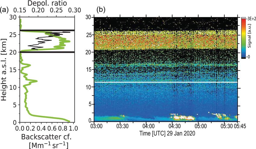
9780                                                                      A. Ansmann et al.: Lidar-based smoke retrievals

ture within a changing global climate with more hot and dry      Müller et al., 2005; Tesche et al., 2011; Alados-Arboledas
weather conditions (Liu et al., 2009, 2014; Kitzberger et al.,   et al., 2011; Veselovskii et al., 2015) as well as in the strato-
2017; Kirchmeier-Young et al., 2019; Dowdy et al., 2019;         sphere (Haarig et al., 2018) and even to a stratospheric vol-
Jones et al., 2020; Witze, 2020).                                canic aerosol observation (Mattis et al., 2010). However, this
    Lidars around the world and in space are favorable in-       sophisticated approach needs lidar observation at multiple
struments to monitor and document high-altitude aerosol          wavelengths of very high quality and is strongly based on di-
layers in the troposphere and lower stratosphere over long       rectly observed particle extinction coefficient profiles which
time periods. This was impressively demonstrated after ma-       are not easy to obtain, especially not during the final phase of
jor volcanic eruptions such as the El Chichón and Mt.            major stratospheric perturbations. The lidar inversion tech-
Pinatubo events (Jäger, 2005; Trickl et al., 2013; Sakai         nique can sporadically provide valuable information about
et al., 2016; Zuev et al., 2019). As main aerosol proxies        the relationship between the optical and microphysical prop-
the measured particle backscatter coefficient and the related    erties of observed aerosol layers and thus can be used to
column-integrated backscatter are used. These optical quan-      check the reliability of applied sun-photometer-based con-
tities allow a precise and detailed study of the decay be-       version factors as shown in Sect. 5.5.
havior of stratospheric aerosol perturbations. Furthermore,         The article is organized as follows. An introduction into
for volcanic aerosol a conversion technique was introduced       the complex chemical, microphysical, morphological, and
to derive climate and air-chemistry-relevant parameters such     optical properties of wildfire smoke and the ability of these
as particle extinction coefficient and related aerosol optical   particles to influence ice formation in clouds is given in
thickness (AOT), mass, and surface area concentration from       Sect. 2. In Sect. 3, we provide an overview of the method-
the backscatter lidar observations (Jäger and Hofmann, 1991;     ological concept, i.e., the way we derive the microphysi-
Jäger et al., 1995; Jäger and Deshler, 2002, 2003). Analo-       cal and cloud-relevant smoke properties from height pro-
gously, such a conversion scheme is needed for the analysis      files of the particle backscatter coefficient. A central role in
of free-tropospheric and stratospheric wildfire smoke layers     the data analysis is played by conversion factors (Mamouri
but is not available yet. The two major stratospheric smoke      and Ansmann, 2016, 2017). The way we determined the
events in 2017 and 2020 motivated us to develop a respective     smoke conversion factors from Aerosol Robotic Network
smoke-related data analysis concept. The technique covers        (AERONET) (Holben et al., 1998) sun photometer observa-
the retrieval of smoke microphysical properties and the es-      tions is described in Sect. 4. Section 5 presents the results
timation of cloud-relevant aerosol properties such as cloud      of the AERONET correlation analysis and the derived set of
condensation nuclei (CCN) and ice-nucleating particle (INP)      conversion parameters for fire smoke as obtained from re-
number concentrations. The focus is on backscatter lidar ob-     spective observations with AERONET sun photometers in
servations at 532 nm, but can easily be extended to 355 and      North America, southern Africa, southern South America,
1064 nm, the other two main laser wavelengths used in at-        and Antarctica. A summary of the studies and an uncertainty
mospheric lidar studies. A preliminary version of the new        analysis is given in Sect. 6. Case studies of observations of
method was already applied to describe the decay of strato-      stratospheric Australian smoke with ground-based Raman li-
spheric perturbation after the major Canadian smoke injec-       dar in Punta Arenas, Chile, in January 2020 and of fresh tro-
tion in the second half of year 2017 (Baars et al., 2019) and    pospheric smoke with the CALIPSO lidar over the United
in recent studies of stratospheric smoke observed over the       States in September 2020 are discussed in Sect. 7. Conclud-
North Pole region with ground-based lidar during the winter      ing remarks are given in Sect. 8.
half year of 2019–2020 (Ohneiser et al., 2021). The retrieval
scheme is easy to handle and applicable to lidar observation
from ground and in space and thus can also be used to eval-      2   Wildfire smoke characteristics
uate measurements acquired by the spaceborne CALIPSO
                                                                 The development of a smoke-related conversion method is
(Cloud-Aerosol Lidar and Infrared Pathfinder Satellite Ob-
                                                                 a difficult task because of the complexity of smoke chemi-
servation) lidar (Winker et al., 2009; Omar et al., 2009;
                                                                 cal, microphysical, and morphological properties. To facil-
Kar et al., 2019), CATS (Cloud-Aerosol Transport System
                                                                 itate the discussions in the next sections, a good knowl-
aboard the International Space Station, ISS) (Proestakis et
                                                                 edge of smoke characteristics is necessary and provided in
al., 2019), and the Aeolus lidar (Reitebuch, 2012; Reitebuch
                                                                 this section. The overview is based on the smoke research
et al., 2020; Baars et al., 2020; Baars et al., 2021), which
                                                                 and discussions presented by Fiebig et al. (2003), Müller
continuously monitor the global aerosol distribution.
                                                                 et al. (2005, 2007a), Dahlkötter et al. (2014), China et al.
    For completeness, alternative lidar techniques are avail-
                                                                 (2015, 2017), Knopf et al. (2018), and Liu and Mishchenko
able to derive microphysical properties of smoke layers from
                                                                 (2018, 2020).
lidar observations (Müller et al., 1999a, 2014; Veselovskii
et al., 2002, 2012). These comprehensive inversion methods
were successfully applied to wildfire smoke layers in the tro-
posphere (Wandinger et al., 2002; Murayama et al., 2004;

Atmos. Chem. Phys., 21, 9779–9807, 2021                                            https://doi.org/10.5194/acp-21-9779-2021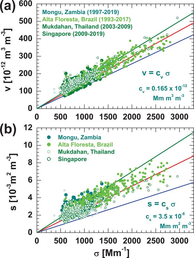
A. Ansmann et al.: Lidar-based smoke retrievals                                                                                9781

2.1   Chemical, physical, and morphological properties               assumed a concentric-spheres core–shell morphology for
                                                                     the strongly-light-absorbing BC core and further assumed
First of all, the types of fires, e.g., flaming versus smoldering    purely-light-scattering coating material (i.e., no absorption
combustion, the fuel type (burning material), and the com-           by the shell) in their analysis of the airborne in situ obser-
bustion efficiency at given environmental and soil moisture          vations. The authors emphasized that their core–shell model
conditions determine the initial chemical composition and            is an idealized scenario because the BC cores of combustion
size distribution of the smoke particles injected into the at-       particles are fractal-like or compact aggregates and BC can
mosphere. Burning of biomass at higher temperatures, dur-            be mixed with light-scattering material in different ways, in-
ing flaming fires, generates smaller particles than smoldering       cluding, e.g., surface contact of BC with the light-scattering
fires (Müller et al., 2005). In forest fires, the flaming stage is   components, full immersion of BC in the light-scattering
usually followed by a longer period of smoldering fires.             component, or immersion of the light-scattering components
   Smoke particles from forest fires are largely composed of         in the BC aggregate. A process that can produce near-surface
organic material (organic carbon, OC) and, to a minor de-            BC morphology is coagulation of almost bare BC aggregates
gree, of black carbon (BC). The BC mass fraction is typi-            with BC-free particles. Condensation of secondary organic
cally < 5 % (Dahlkötter et al., 2014; Yu et al., 2019) but may       or inorganic aerosol components on BC particles can result
reach values of 10 %–15 % in cases of complex mixtures of            in particles either with core–shell morphology (concentric
anthropogenic haze with domestic, forest, and agricultural           or eccentric) or with near-surface BC morphology. All these
fire smoke (Wang et al., 2011). Biomass burning aerosol also         possible morphology features must be considered in the dis-
consists of humic-like substances (HULIS), which represent           cussion and estimation of the smoke optical properties and
large macromolecules (Mayol-Bracero et al., 2002; Schmidl            of the potential of smoke particles to serve as INP (Sects. 2.2
et al., 2008a, b; Fors et al., 2010; Graber and Rudich, 2006).       and 3.1).
The particles and released vapors within biomass burning                Changes in the morphology (size, shape, and internal
plumes undergo chemical and physical aging processes dur-            structure) of smoke particles and their internal mixing state
ing long-range transport. There is strong evidence from lidar        (e.g., soot particle coating) are ongoing during long-range
observations that smoke particles grow in size during the ag-        transport. As China et al. (2015) pointed out, freshly emitted
ing phase (Müller et al., 2007a). Processes that lead to the in-     soot particles, i.e., BC particles, are typically hydrophobic,
crease in particle size are hygroscopic growth of the particles,     lacy fractal-like aggregates of carbonaceous monomers and
gas-to-particle conversion of inorganic and organic vapors           become hydrophilic as a result of coating and other aging
during transport, condensation of large organic molecules            processes. Lace soot undergoes compaction upon humidifi-
from the gas phase in the first few hours of aging, coagula-         cation. All these effects lead to an increased ability of smoke
tion, and photochemical and cloud-processing mechanisms.             particles to serve as CCN with increasing long-range travel
The lidar observations are in agreement with modeling stud-          time.
ies of Fiebig et al. (2003), who used the theory of particle            Soot compaction (and collapse of the core structures)
aging processes described by Reid and Hobbs (1998). Con-             changes also the scattering and absorption cross sections de-
densational growth dominates the increase in particle size in        pending on the refractive index, the monomer diameter, and
the first 2 d after emission of a plume. Thereafter coagulation      the structural details. Many publications dealing with the op-
in the increasingly diluted plumes becomes the dominating            tical properties became available in recent years (China et al.,
process. A significant shift of the particle size distribution       2015; Liu and Mishchenko, 2018, 2020; Kahnert, 2017; Yu
indicated by an increase in the number median radius from            et al., 2019; Gialitaki et al., 2020). Liu and Mishchenko
about 0.2 µm shortly after emission to about 0.35 µm after 6 d       (2018) mentioned that their model considers 11 different
of travel was found in several cases of Canadian smoke by            model morphologies ranging from bare soot to completely
Müller et al. (2007a). The aging effect has to be considered         embedded soot–sulfate and soot–brown carbon mixtures. In
in the retrieval of smoke conversion factors. We distinguish         agreement with earlier studies, they found that for the same
fresh and aged smoke observations in Sect. 5.                        amount of absorbing material, the absorption cross section
   Dahlkötter et al. (2014) analyzed aircraft in situ mea-           of internally mixed soot can be more than twice that of bare
surements of a smoke layer advected from North America               soot. Thus absorption increases as soot accumulates more
and observed over Germany at 10–12 km height in Septem-              coating material during long-range transport. As a general
ber 2011 and found, in agreement with many other airborne            finding of the modeling studies, the absorption enhancement
in situ observations, an almost monomodal size distribution          is a complex function of many factors such as the size and
of smoke particles with a pronounced accumulation mode               shape of the soot aerosols, the mixing state, the location of
(particles with diameters from roughly 200 to about 1400 to          soot within the host, and the amount and composition of the
1800 nm). A distinct coarse mode was absent.                         coating material. All these facts make it necessary to distin-
   The black-carbon-containing smoke particles showed                guish between fresh smoke (2.5 d of long-range transport) in our at-
diameter ratios of typically 2–3. Dahlkötter et al. (2014)           tempt to determine smoke conversion parameters.

https://doi.org/10.5194/acp-21-9779-2021                                              Atmos. Chem. Phys., 21, 9779–9807, 2021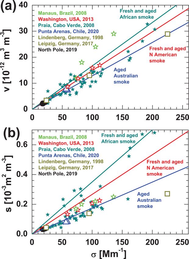
9782                                                                          A. Ansmann et al.: Lidar-based smoke retrievals

2.2    Cloud-relevant properties                                        However, in reality, at given air mass lifting conditions,
                                                                     the ice nucleation process can be very complex. The time that
As already mentioned, smoke particles after long-range               solid OM needs for transition to a more liquid state, termed as
transport seem to be favorable CCN because they become               humidity-induced amorphous deliquescence, can range from
increasingly hydrophilic during aging. In contrast to the im-        several minutes to days at temperatures low enough for ice
pact of smoke on cloud droplet formation, the characteriza-          formation (Mikhailov et al., 2009; Berkemeier et al., 2014;
tion of their influence on ice nucleation is rather difficult. The   Knopf et al., 2018). Thus the phase change (as function of T
link between ice nucleation efficiency and particle chemical         and RH) can be longer than typical cloud activation time pe-
and morphological properties and the ongoing modifications           riods (governed by the updraft velocity), potentially inhibit-
of the properties during long-range transport is largely unre-       ing full deliquescence and allowing the OA or the organic
solved (China et al., 2017). However, it is widely assumed           coating to serve as INP. When amorphous OA or OM are in-
that the ability of smoke particles to serve as INP mainly de-       volved in ice nucleation, the condensed-phase diffusion pro-
pends on the organic material (OM) in the shell of the coated        cesses within OA particles will most probably govern the ice
smoke particles (Knopf et al., 2018). BC is not considered           nucleation pathway (Wang et al., 2012).
to be an important contributor to immersion freezing (Möh-              The following potential scenarios of atmospheric ice nu-
ler et al., 2005; Ullrich et al., 2017; Schill et al., 2020; Kanji   cleation are uniquely attributable to the presence of amor-
et al., 2020), which is assumed to be the preferred heteroge-        phous OM. (1) Ice formation in the glassy region may be
neous ice nucleation mode.                                           due to ice nucleation on the solid organic particle, i.e., de-
   Knopf et al. (2018) present a review on the role of or-           position ice nucleation. (2) During partial deliquescence, a
ganic aerosol (OA) and OM in atmospheric ice nucleation. A           residual solid core is coated by an aqueous shell, and im-
unique feature of OA particles is that they can be amorphous         mersion freezing may proceed. (3) At full deliquescence RH,
and can exist in different phases, including liquid, semisolid,      where the particles are completely liquid (and contain no
and solid (or glassy) states, in response to changes in tem-         solid soot fragments), homogeneous freezing will occur at
perature (T ) and relative humidity (RH) (Koop et al., 2011;         temperatures below about 238 K. (4) The presence of a glassy
Zobrist et al., 2008; Knopf et al., 2018). At low temperatures,      phase in disequilibrium with surrounding water vapor (e.g.,
e.g., in the UTLS region, where the atmospheric temperature          cloud activation at fast updrafts as discussed below) may sup-
can be as low as 180 K, it is conceivable to assume that the         press or initiate ice nucleation beyond the homogeneous ice
particles are in a glassy state. Most of the secondary organic       nucleation limit (Berkemeier et al., 2014; Knopf et al., 2018).
aerosol particles are solid above 500 hPa (about 5 km) ac-           A slower updraft velocity allows for more time for deliques-
cording to modeling studies and for temperatures < 240 K             cence to proceed, potentially resulting in full deliquescence
(Shiraiwa et al., 2017).                                             of the OA particle at warmer and drier conditions compared
   It has been shown that humic and fulvic matter can act as         to when a faster updraft is active. Therefore, the same OM
deposition nucleation and immersion freezing INPs (Wang              can be present in different phase states under the same atmo-
and Knopf, 2011; Rigg et al., 2013; Knopf and Alpert, 2013;          spheric thermodynamic conditions (i.e., T and relative hu-
Knopf et al., 2018). Furthermore, these macromolecules can           midity over ice RHi ), resulting in different ice nucleation
undergo amorphous phase transition under typical tropo-              pathways and corresponding ice nucleation rates. OA particle
spheric conditions (Wang et al., 2012; Slade et al., 2017)           size or coating thickness can also impact the rate and atmo-
similar to the processes we assume the organic coating of            spheric altitude of the organic phase change, as larger parti-
the smoke particles experience.                                      cles or thicker coatings require more time to reach full deli-
   Aerosol particles serving as INPs usually provide an in-          quescence (Charnawskas et al., 2017). There are many more
soluble, solid surface that can facilitate the freezing of wa-       peculiarities of amorphous OM that make INP parameteriza-
ter (Knopf et al., 2018). Deposition ice nucleation is defined       tion and prediction efforts very complicated as discussed in
as ice formation occurring on the INP surface by water va-           detail by Knopf et al. (2018).
por deposition from the supersaturated gas phase. Although,             Since amorphous smoke OA may take up water and par-
recent studies suggest that deposition ice nucleation can be         tially deliquesce, resulting in an aqueous solution at possibly
the result of pore condensation freezing, where homogeneous          subsaturated conditions, we apply the water-activity-based
ice nucleation occurs at lower supersaturation in nanometer-         immersion freezing (ABIFM) parameterization (Knopf and
sized pores (David et al., 2019; Marcolli, 2014). When the           Alpert, 2013; Alpert and Knopf, 2016) and homogeneous ice
supercooled smoke particle takes up water or its shell deli-         nucleation parameterization by Koop et al. (2000). ABIFM
quesces, immersion freezing can proceed, where the INP im-           derives the number of INPs per volume of air for a given
mersed in an aqueous solution can initiate freezing (Knopf           time period, when T , RH, and particle surface area s are
et al., 2018; Berkemeier et al., 2014). Finally, if the smoke        known (see Sect. 3.1.1). A deposition ice nucleation scheme
particle becomes completely liquid (and no insoluble part            based on classical nucleation theory is outlined in addition
within the particle is left), homogeneous freezing will take         (Sect. 3.1.3) to cover the potential pathway of glassy smoke
place at temperatures below 235 K (Koop et al., 2000).

Atmos. Chem. Phys., 21, 9779–9807, 2021                                               https://doi.org/10.5194/acp-21-9779-2021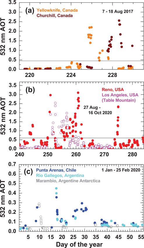
A. Ansmann et al.: Lidar-based smoke retrievals                                                                              9783

particles to serve as INPs. Again, T , RH, and s are input in      suming a low smoke depolarization ratio of  0.9) in the UTLS regime, and the
optical into microphysical particle properties is given by         soil dust fraction can be neglected at these heights.
Mamouri and Ansmann (2016, 2017). It is out of the scope of           To obtain height profiles of smoke in terms of volume
this article to present a detailed approach of how an aerosol      concentration v(z), surface area concentration s(z), particle
layer can be unambiguously identified and classified as a          number concentrations n50 (z), considering all particles with
smoke layer. In case of single-wavelength backscatter li-          radius > 50 nm, and the large-particle number concentration
dars, backward trajectory analysis is the main tool to iden-       n250 (z), considering particles with particle radius > 250 nm,
tify smoke layers and link them to the most probable fire          we have the following four basic relationships:
source region. In the case of modern aerosol lidars equipped
with polarization-sensitive channels and aerosol and molec-        v(z) = cv Lβ(z) ,                                           (1)
ular backscatter channels at several wavelengths, favorable        s(z) = cs Lβ(z) ,                                           (2)
conditions are given to identify smoke layers based on the         n250 (z) = c250 Lβ(z) ,                                     (3)
complex set of available information on particle backscatter       n50 (z) = c50 [Lβ(z)]x ,                                    (4)
and extinction coefficients, depolarization ratio, and lidar ra-
tio (Wandinger et al., 2002; Müller et al., 2005; Tesche et        with the particle backscatter coefficient β(z) at height z and
al., 2011; Burton et al., 2012, 2015; Giannakaki et al., 2015;     the extinction-to-backscatter or lidar ratio L. The needed
Giannakaki et al., 2016; Prata et al., 2017; Haarig et al.,        conversion factors cv , cs , c250 , and c50 and the extinc-
2018; Hu et al., 2019; Adam et al., 2020; Ohneiser et al.,         tion exponent x for 532 nm are obtained from the analysis
2020, 2021). However, an unambiguous and accurate quan-            of AERONET observations during situations dominated by
tification of the smoke fraction or contribution to the mea-       wildfire smoke. The results of our smoke-related AERONET
sured optical backscatter and extinction properties and the        data analysis are presented in Sect. 5.
separation of smoke and soil dust fractions remains difficult.        An important input parameter is the smoke lidar ratio L,
Soil dust may have been injected together with the smoke by        required to obtain the smoke extinction coefficient σ = Lβ
the hot fires.                                                     in the first step of the conversion procedure. As discussed
    Regarding the separation of smoke and dust fractions by        in the review of Adam et al. (2020), the smoke lidar ratio
means of the polarization lidar technique (Tesche et al.,          can vary from 25 to 150 sr at 532 nm. However, most stud-
2009, 2011; Nisantzi et al., 2014), we have to distinguish         ies show that the 532 nm lidar ratio is typically in the range
two branches. As long as the smoke-containing layers oc-           of 70 sr ± 25 sr. For 355 nm, lidar ratios were mostly found
cur at low altitudes (in the lower and middle troposphere up       around 75 ± 25 sr for fresh smoke and 55 ± 20 sr for aged
to 5–7 km height), we can apply the traditional approach to        smoke. Table 1 provides an overview of the large range of
determine the smoke fraction in dust–smoke mixtures by as-         smoke lidar ratios. Aged smoke shows a characteristic L ra-

https://doi.org/10.5194/acp-21-9779-2021                                            Atmos. Chem. Phys., 21, 9779–9807, 2021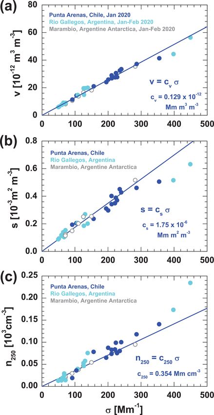
9784 A. Ansmann et al.: Lidar-based smoke retrievals
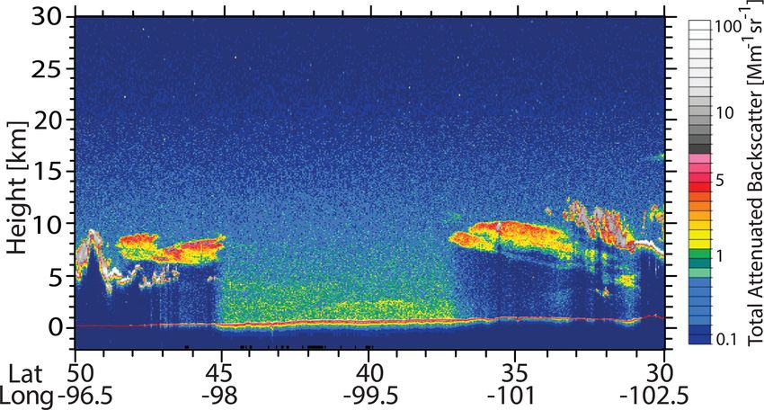
Figure 1. Australian bushfire smoke (yellow layer) in the stratosphere, almost 10–15 km above the tropopause (white line in b). The mean
backscatter coefficient profile (green) and the particle depolarization-ratio profile (black, for the main layer only) for the 165 min observation
are shown in the left panel. Main smoke layer base and top height are indicated by black horizontal lines in panel (a). The smoke was
observed with lidar at Punta Arenas, Chile, on 29 January 2020, about 10 000 km downwind of the Australian fire areas. The range-corrected
1064 nm lidar return signal is shown.
tio of L355 nm /L532 nm < 1. This feature allows a clear unam- reviewed the smoke research in China and concluded that the
biguous identification of smoke layers after long-range trans- smoke particle density is 1.0–1.9 g cm−3 . Thus in cases with
port (Müller et al., 2005; Noh et al., 2009; Nicolae et al., 2 %–10 % of BC the overall smoke particle density should be
2013; Ohneiser et al., 2020). The reason for the large spec- in the range of 1.0–1.3 g cm−3 .
trum of lidar ratios is the complex smoke properties (size, The particle concentration n50 is a good aerosol proxy
shape, composition) as discussed in Sect. 2. Extended dis- for aerosol particles serving as cloud condensation nuclei
cussions on smoke lidar ratios can be found in Nicolae et al. (CCN),
(2013), Haarig et al. (2018), and Adam et al. (2020).
We recommend to use a lidar ratio of 55 sr for 355 nm nCCN,Sw =0.2 % (z) = n50 (z) . (6)
and 70 sr for 532 nm for aged smoke if there is no possibil- The CCN concentration is a strong function of updraft speed
ity to obtain actual lidar ratio information from Raman li- and thus water supersaturation Sw . The number concentra-
dar (Wandinger et al., 2002; Veselovskii et al., 2015; Haarig tion n50 roughly indicates the CCN concentration for weak
et al., 2018; Ohneiser et al., 2020, 2021) or High Spectral updrafts and frequently observed low water supersaturations
Resolution Lidar (HSRL) observations (Wandinger et al., of Sw = 0.2 %. Water supersaturation values may be in the
2002; Burton et al., 2015), or in the way Prata et al. (2017) range of 0.4 %–0.7 % in strong updrafts. Then the CCN con-
proposed in the case of the CALIPSO lidar to estimate the centration is a factor of about 2 higher than n50 .
lidar ratio of smoke layers embedded in clear air. For fresh In the case of free-tropospheric and stratospheric smoke,
smoke, an appropriate value for the lidar ratio seems to be we assume that the relative humidity in the smoke plumes is
70-80 sr at both wavelengths. typically < 60 % so that the derived n50 values represent the
From the obtained values of v, s, and n50 further relevant number concentrations for dry aerosol particles, required in
parameters can be calculated. The smoke mass concentration the CCN estimation. The estimation of CCN concentration in
m is given by cases with high relative humidity and corresponding aerosol
water-uptake effects is described in Mamouri and Ansmann
m(z) = ρv(z) , (5) (2016).
The particle concentration n250 indicates the reservoir of
with ρ the density of the smoke particles. Li et al. (2016) favorable INPs and is even used as input in dust-INP param-
investigated different smoke aerosols in the laboratory by eterizations (DeMott et al., 2015). However, in the case of
burning of different straw types and found densities of 1.1 smoke the input parameter in the INP retrieval is the surface
to 1.4 g cm−3 for the produced smoke particles. For organic area concentration s,
particles ρOM was about 1.05 ± 0.15 g cm−3 , and for ρEC (el-
emental carbon) they yielded 1.8 g cm−3 . Chen et al. (2017) nINP (z) = f (s(z), Si (z), T (z)) . (7)
Atmos. Chem. Phys., 21, 9779–9807, 2021 https://doi.org/10.5194/acp-21-9779-2021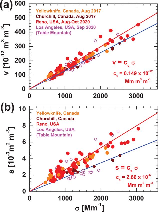
A. Ansmann et al.: Lidar-based smoke retrievals                                                                                       9785

Table 1. Dual-wavelength lidar observations of lidar ratios (L) at 355 and 532 nm in tropospheric (T) and stratospheric (S) smoke layers.

                        Atmospheric layer              L(355 nm)     L(532 nm)      Reference
                        Aged Canadian smoke (S)        35–50 sr      50-80 sr       Haarig et al. (2018)
                        Aged Australian smoke (S)      50–95 sr      70–110 sr      Ohneiser et al. (2020)
                        Aged Canadian smoke (T)        65 sr         90 sr          Wandinger et al. (2002)
                        Aged Siberian smoke (T)        40 sr         65 sr          Murayama et al. (2004)
                        North American smoke (T)       65–90 sr      65–80 sr       Veselovskii et al. (2015)
                        European smoke (T)             60–65 sr      60–65 sr       Alados-Arboledas et al. (2011)
                        European smoke (T)             30–60 sr      45–65 sr       Nicolae et al. (2013)
                        European smoke (T)             40–105 sr     40–110 sr      Mylonaki et al. (2018)
                        Amazonian smoke (T)            50–75 sr      50–80 sr       Baars et al. (2012)
                        Western African smoke (T)      50–110 sr     50–105 sr      Tesche et al. (2011)
                        South African smoke (T)        70–110 sr     60–105 sr      Giannakaki et al. (2015)

The INP concentration is a function of s, the ice supersat-             conditions) are scarce (Knopf et al., 2018). Knopf and Alpert
uration Si (which occurs during lifting processes), and tem-            (2013) introduced the water-activity-based immersion freez-
perature T . Details of the complex INP parameterization are            ing model ABIFM, drawn from the water-activity-based ho-
given in Sect. 3.1.                                                     mogeneous ice nucleation theory (Koop et al., 2000). Knopf
   Finally, information on smoke particle number concentra-             and Alpert (2013) present an ABIFM parameterization for
tions (n50 , n250 ) and surface area concentration s at strato-         two types of humic compounds based also on experimental
spheric heights is of interest in studies of heterogeneous for-         data by Rigg et al. (2013) that is valid for saturated and sub-
mation of polar stratospheric clouds (PSCs). A significant              saturated atmospheric conditions. For demonstration of our
increase in smoke aerosol particle concentration may have               method, we chose to apply the ABIFM for leonardite (a stan-
a sensitive impact on the evolution of PSCs and their micro-            dard humic acid surrogate material) to represent the amor-
physical properties (Voigt et al., 2005; Hoyle et al., 2013;            phous organic coating of smoke particles. The ABIFM al-
Engel et al., 2013; Zhu et al., 2015).                                  lows prediction of the ice particle production rate Jhet,I as
   In order to use the developed smoke retrieval formalism              a function of ambient air temperature T (freezing tempera-
presented here in the case of backscatter lidars operated at            ture), ice supersaturation Si , particle surface area s, and time
single wavelengths of λ = 355 or 1064 nm backscatter li-                period 1t for which a certain level of ice supersaturation Si is
dars, we need to estimate the respective backscatter coeffi-            given. For demonstration purposes, we simply assume a con-
cient at 532 nm in the first step. The 532 nm backscatter pro-          stant supersaturation period 1t of 10 min (600 s). Such su-
files within smoke layers may be estimated by using typical             persaturation conditions may occur during the upwind phase
smoke color ratios β(532 nm)/β(λ). This aspect is further               of a gravity wave.
discussed in Sect. 6.                                                      According to Eqs. (6)–(8) in Alpert and Knopf (2016), we
                                                                        calculate the so-called water activity criterion (Koop et al.,
3.1     INP parameterization                                            2000) in the first step:
As discussed in Sect. 2.2, the estimation of INP concentra-             1aw = aw − aw,i (T ) .                                          (8)
tions is challenging due to the chemical complexity of the
smoke aerosol. The parameterizations introduced in this sec-            The term aw,i in Eq. (8),
tion cover the OM-related ice nucleation for the temperature
range in the upper troposphere (< −40 ◦ C). Only for these              aw,i = Pi (T )/Pw (T ),                                         (9)
low temperatures, organic smoke particles may be able to in-
fluence ice nucleation in the atmosphere. In the following,             is the ratio of ice saturation pressure Pi to water saturation
we present procedures to compute INP concentrations for                 pressure Pw as function of temperature T and can be ac-
immersion freezing, deposition ice nucleation, and homoge-              curately determined by using Eq. (7) in Koop and Zobrist
neous freezing.                                                         (2009). When the condensed phase and vapor phase are in
                                                                        equilibrium, the water activity aw is equal to RHw (written
3.1.1    Immersion freezing                                             as 0.75 if RHw = 75 %) in the air parcel in which ice nucle-
                                                                        ation takes place (e.g., in a cirrus layer at height z at tem-
Organic smoke particles that have undergone long-range                  perature T ). Relative humidity and temperature values may
transport are chemically complex, and INP parameterizations             be available from radiosonde ascents or taken from databases
that capture the ice formation rate at upper tropospheric and           with re-analyzed global atmospheric data. However, the ac-
lower stratospheric conditions (i.e., including subsaturated            tual RHw and T values during the lifting process (associated

https://doi.org/10.5194/acp-21-9779-2021                                                   Atmos. Chem. Phys., 21, 9779–9807, 2021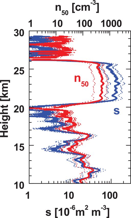
9786                                                                        A. Ansmann et al.: Lidar-based smoke retrievals

with cooling and increase in RHw and decrease in T in the air      homogeneous freezing is obtained from
parcel) remain always unknown and need to be estimated in
the studies of a potential smoke impact on cirrus formation.       log10 (Jhom ) = −906.7 + 85021aw − 26924(1aw )2
The organic aerosol type leonardite needs a relative humid-                    + 29180(1aw )3                                (12)
ity over ice RHi of about 130 % or 1aw = 0.2 at −50 ◦ C to
become efficiently activated as INP.                               for 0.26 < 1aw < 0.34. The INP concentration is then ob-
   In the next step, the ice crystal nucleation rate coefficient   tained from
Jhet,I (in cm−2 s−1 ) is calculated:
                                                                   nINP,hom = vJhom 1t,                                      (13)
log10 (Jhet,I ) = b + k1aw .                               (10)
                                                                   with the particle volume concentration v in cm3 m−3 . Ho-
The particle parameters b and k are determined from lab-           mogeneous freezing proceeds at RHi ≈ 150 % at −50 ◦ C
oratory studies for different organic aerosol material. Ta-        (i.e., 1aw ≈ 0.31), whereas 130 % (1aw = 0.2) is required
ble 2 contains the parameters for two different natural or-        at −50 ◦ C to activate leonardite-containing particles. Thus
ganic substances (Pahokee peat and leonardite) (Knopf and          at slow ascent conditions heterogeneous ice nucleation on
Alpert, 2013) which serve as surrogates of the organic coat-       smoke particles may dominate ice formation in cirrus layers.
ing of the atmospheric smoke particles. Leonardite, an ox-
idation product of lignite, is a humic-acid-containing soft        3.1.3   Deposition nucleation
waxy particle (mineraloid), black or brown in color, and sol-
uble in alkaline solutions. Both substances served as surro-       Wang and Knopf (2011) provide a simplified parameteriza-
gates for humic-like substances (HULIS, Sect. 2.1) in ex-          tion of deposition ice nucleation (DIN) based on classical
tended immersion freezing laboratory studies (Knopf and            nucleation theory that describes the DIN efficiency of humic
Alpert, 2013; Rigg et al., 2013). Organic aerosols contain-        and fulvic acid compounds as a function of ambient temper-
ing HULIS are ubiquitous in the atmosphere. We also applied        ature T and the humidity parameters RHi and Si . An alterna-
the ABIFM parameterization to aerosol samples representing         tive DIN parameterization is provided by, e.g., Hoose et al.
free-tropospheric aerosol (FTA, China et al., 2017) collected      (2010). A detailed description of the approach presented here
on substrates on the Azores for offline micro-spectroscopic        is given in Sect. 3.6 in Wang and Knopf (2011), and thus only
single-particle analysis and ice nucleation experiments. Ac-       a brief introduction is given in the following.
cording to backward trajectories, the air masses arriving at          The INP efficiencies are expressed as a function of the
the Azores crossed western parts of North America during           contact angle 2, which describes the relationship of surface
the main fire season (August–September). FTA showed clear          free energies among the three involved interfaces including
smoke signatures. Note that Eq. (10) delivers strongly fluc-       water vapor, ice embryo, and INP. 2 is parameterized as a
tuating solutions of Jhet,I when 1aw is small, and it delivers     function of RHi (Eq. 8 in Wang and Knopf, 2011).
robust, less fluctuating Jhet,I values for 1aw > 0.1.                 The compatibility parameter m2 = cos(2) (expressing
   In the final step, we obtain the number concentration of        the match between ice embryo and INP) is then used to deter-
smoke INP for the immersion freezing mode,                         mine the so-called geometric factor fg (m2 ) (Eq. 7 in Wang
                                                                   and Knopf, 2011), the free energy of ice embryo formation
                                                                   1Fg,het (fg , T , Si ) (Eq. 6 in Wang and Knopf, 2011), and fi-
nINP,I = sJhet,I 1t,                                       (11)
                                                                   nally the ice crystal nucleation rate Jhet,D (Eq. 5 in Wang and
                                                                   Knopf, 2011) in cm−2 s−1 ,
with the surface area concentration s of the smoke particles
in cm2 m−3 and the time period 1t (in seconds) for which
                                                                                           −1Fg,het

constant or almost constant ice supersaturation conditions are     Jhet,D = 1025 exp                   ,                      (14)
                                                                                             kB T
given. This can be the time period of a short updraft event
(of a few minutes, 120–300 s) or of the lifting period of a        with the Boltzmann constant kB . The final step is then
gravity wave (>600 s). Long-lasting lifting phases of gravity
waves can be up to 20 minutes (1200 s) as our Doppler lidar        nINP,D = sJhet,D 1t .                                     (15)
and radar observations conducted in several field campaigns
during the last 10 years indicate.                                    In terms of the contact-angle-based approach, 2 = 180◦
                                                                   represents the case of homogeneous ice nucleation. The
3.1.2   Homogeneous freezing                                       smaller 2, the greater the propensity of the INP to act as
                                                                   deposition nucleation INP.
Alternatively to smoke particles acting as heterogeneous              At the end of this section it remains to be emphasizes that
INPs, we need to consider full deliquescence of smoke parti-       we put together several INP parameterizations in Sect. 3.1
cles so that homogeneous freezing comes into play. Follow-         for demonstration purposes. The research on the smoke im-
ing Koop et al. (2000), the ice nucleation rate coefficient for    pact on atmospheric ice formation is ongoing (Knopf et al.,

Atmos. Chem. Phys., 21, 9779–9807, 2021                                             https://doi.org/10.5194/acp-21-9779-2021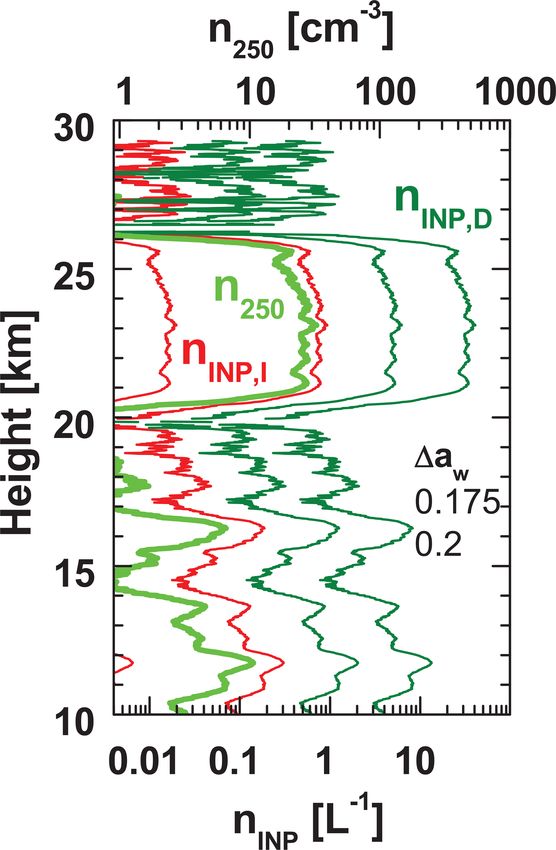
A. Ansmann et al.: Lidar-based smoke retrievals                                                                                         9787

Table 2. Values for b and k for three organic aerosol INP types required to determine the ice nucleation rate Jhet,I with Eq. (10).

                  INP type                                                          b        k    Reference
                  Pahokee peat (organic substance)                            −15.78     78.31    Knopf and Alpert (2013)
                  Leonardite (organic substance)                              −13.40     66.90    Knopf and Alpert (2013)
                  Free-tropospheric aerosol (smoke plumes over Azores)         0.656     2.981    China et al. (2017)

2018). Presently, uncertainties in the prediction of Jhet,I and
Jhet,D for organic aerosols are very high (Wang and Knopf,
2011; China et al., 2017). However, the procedures intro-
duced above allow us to estimate INP concentration pro-
files for organic aerosols and to study the potential impact
of wildfire smoke on ice formation in tropospheric mixed-
phase and ice clouds. In the upcoming years, strong field
activities are required, including comparisons of airborne
in situ with lidar observations of smoke INP concentra-
tions as successfully performed in the case of Saharan dust
(Schrod et al., 2017; Marinou et al., 2019) and so-called
cirrus closure experiments as realized in the case of cirrus              Figure 2. AERONET stations used in our study. Aged stratospheric
formation in pronounced Saharan dust layers (Ansmann et                   smoke from the major Australian bush fires was observed over the
al., 2019b) in order to check the applicability of developed              South American and Antarctic stations (Rio Gallegos, Punta Are-
smoke INP parameterizations and to quantify the uncertain-                nas, Marambio) in January and February 2020. Fresh and aged
                                                                          stratospheric smoke from record-breaking fires in British Columbia,
ties in the INP estimates under real-world meteorological,
                                                                          Canada, were measured over Yellowknife and Churchill, respec-
cloud, and aerosol conditions. A first closure study with re-
                                                                          tively, in August 2017. Mixtures of fresh and aged tropospheric
spect to smoke–cirrus interaction was recently presented by               smoke originating from strong fires in the western United States and
Engelmann et al. (2020).                                                  Canada were found over Reno and Table Mountain in late August
                                                                          to mid-October 2020. AERONET stations at Alta Floresta, Mongu,
                                                                          Mukdahan, and Singapore have long, multiyear data records of
4     AERONET sites and data analysis                                     smoke observations in key regions of biomass burning.

The AERONET database (AERONET, 2021) contains
unique multiyear climatological data sets of spectrally re-
solved aerosol optical properties and related underlying mi-              plumes, for different fire types and burning material, and
crophysical properties of aerosol particles (e.g., size dis-              smoke occurrence in the troposphere and stratosphere.
tribution, volume, and surface area concentration). These                    Yellowknife (AERONET site: Yellowknife Aurora) and
AERONET products are available in the database for purely                 Churchill in Canada were selected because these AERONET
marine, dust, biomass-burning smoke, and anthropogenic                    sites were located in the outflow region of major smoke
haze conditions as well as for complex mixtures of these ba-              plumes which originated from the record-breaking wildfires
sic aerosol types. We used the advantage of the AERONET                   in British Columbia (Hu et al., 2019; Baars et al., 2019;
database already to derive the conversion parameters for ma-              Torres et al., 2020), Canada, in August 2017. Strong py-
rine and Saharan dust conditions (Mamouri and Ansmann,                    rocumulonimbus (pyroCb) towers (Fromm et al., 2010) de-
2016, 2017) and extended the dust-related study later on                  veloped and lifted enormous amounts of wildfire smoke
to many desert dust regions around the world (Ansmann et                  into the upper troposphere and lower stratosphere (UTLS)
al., 2019a). Now, we apply the methodology to the wildfire                from 21:00 UTC on 12 August to 00:30 UTC on 13 Au-
aerosol type.                                                             gust 2017 (Peterson et al., 2018). The smoke observation at
                                                                          Yellowknife and Churchill could be thus well assigned to the
4.1    AERONET sites                                                      time after injection and allowed us to study the change in
                                                                          the smoke conversion parameters as a function of time from
The smoke conversion parameters cv , cs , c50 , c250 , and x,             12–18 h to about 5 d after injection.
required to solve Eqs. (1)–(4), were determined from sun                     The AERONET stations at Rio Gallegos (CEILAP-RG),
photometer observations at nine AERONET stations, dis-                    Argentina; Punta Arenas (Punta-Arenas-UMAG), Chile, at
tributed over several continents. Figure 2 shows the con-                 the southernmost tip of South America; and Marambio
sidered AERONET stations. The observations at these sites                 in Antarctica were selected because well-aged smoke lay-
cover the full range of smoke scenarios, from fresh to aged               ers crossed these stations in January and February 2020

https://doi.org/10.5194/acp-21-9779-2021                                                    Atmos. Chem. Phys., 21, 9779–9807, 2021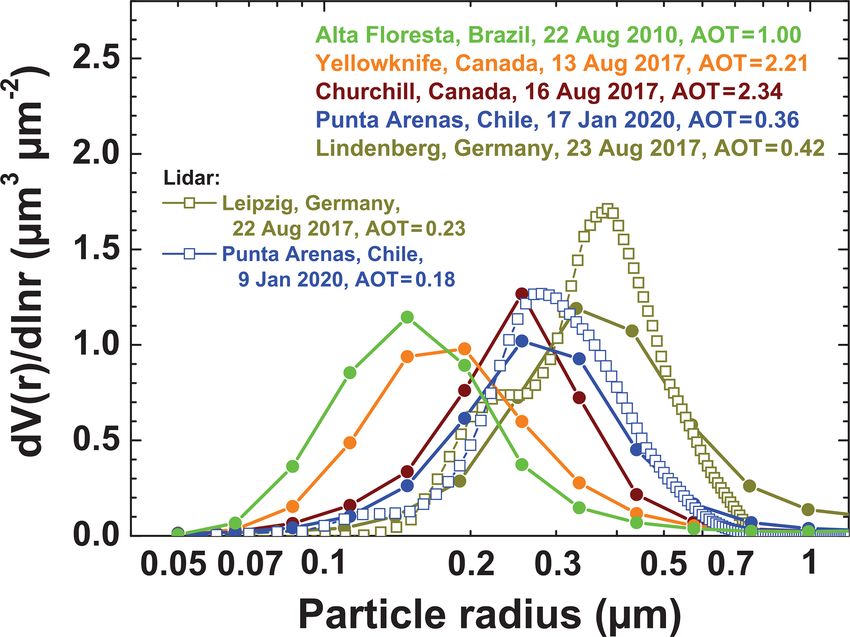
9788                                                                       A. Ansmann et al.: Lidar-based smoke retrievals

(Ohneiser et al., 2020). The smoke originated from strong         particle backscatter coefficients at six wavelength (355, 400,
fires in southeastern Australia and traveled the 10 000 km dis-   532, 710, 800, 1064 nm) and extinction coefficients at 355
tance within 8–12 d. Strong pyroCb activity lifted the smoke      and 532 nm were available (Wandinger et al., 2002).
layers up to UTLS heights, and self-lifting processes (Boers
et al., 2010) caused further ascent to heights 10–20 km above     4.2   AERONET data analysis
the tropopause (Ohneiser et al., 2020; Kablick et al., 2020;
Khaykin et al., 2020). The background AOT levels are clearly      We used the version-3 level-2.0 inversion AERONET prod-
below 0.05 at 532 nm at these high northern and southern          ucts (AERONET, 2021) in the case of the long-term obser-
mid-latitudinal stations, far away from industrialized centers,   vations in the Amazon region, southern Africa, and South-
so that the smoke layers could be clearly identified and dom-     east Asia and level-1.5 data in the case of the remaining
inated the sun photometer observations over many days (Yel-       stations. The reason for using level-1.5 data was to signifi-
lowknife, Churchill) and weeks (Punta Arenas, Rio Gallegos,       cantly increase the number of available observations in our
Marambio).                                                        smoke-related studies. Many observations showing high to
   In order to consider several centers of biomass burning of     very high smoke AOTs could not pass the strict criteria of the
global importance we selected six further AERONET sta-            AERONET data quality checks and were thus removed from
tions. Smoke from exceptionally strong forest fires in the        the level-2.0 data set. We compared the level-2.0 AERONET
western United States and western Canada was observed             products with the corresponding (reduced) level-1.5 products
over Reno (University of Nevada, Reno), Nevada, and Table         to guarantee that the used level-1.5 data set was of high qual-
Mountain (Table Mountain, CA), California, from the end           ity.
of August to mid-October 2020 (in close distance to the fire         In agreement with the AERONET data analysis of Sayer
sources) and allowed the determination of conversion param-       et al. (2014), we used the fine-mode AOTs stored in the
eters for very fresh and mixtures of fresh and aged North         AERONET database. Smoke particles form a well-developed
American tropospheric smoke layers.                               accumulation mode (with sizes up to about 1 µm in radius)
   We downloaded long-term observations performed at the          and the related optical properties are assigned as fine-mode
AERONET stations Alta Floresta, Brazil (Amazonian forest          AERONET products (Sayer et al., 2014). However, as will be
fires); Mongu, Zambia, in southern Africa; Mukdahan, Thai-        discussed in Sect. 5.1, a bimodal distribution (accumulation
land; and Singapore in Southeast Asia to consider observa-        plus coarse mode) was often retrieved from the AERONET
tions in key fire areas of global importance. The Mongu data      sun and sky observations. This was also pointed out by Sayer
sets consists of sun photometer observations at the Mongu         et al. (2014). The second mode is probably related to soil,
site from 1997–2009 and at the Mongu Inn site from 2013–          road, and desert dust or marine aerosol in the planetary
2019. Fairly constant burning conditions are given at Mongu       boundary layer. The comparison with respective lidar obser-
from July to November of each year. The long-term obser-          vations clearly indicates that smoke produces a pronounced
vations in the Amazon region, southern Africa, and South-         accumulation mode only. A coarse mode is absent. Thus, we
east Asia cover smoldering and flaming fires, fresh and aged      computed the smoke-related values of s, v, n50 , and n250
smoke layers, and agricultural, grassland, savannah, peat,        from the downloaded size distributions by considering the
forest, and bush fires. The selection of these AERONET sta-       size classes 1–11 only (covering the accumulation mode and
tions in key burning areas was guided by the smoke study of       thus the radius range up to 0.9–0.95 µm) and correlated these
Sayer et al. (2014).                                              calculated microphysical values with the fine-mode AOT at
   The AERONET smoke studies are supplemented by mul-             532 nm as stored in the AERONET database to finally obtain
tiwavelength lidar observations of smoke conversion param-        the conversion parameters. Details of the computation of s,
eters. These vertically resolved observations were performed      v, n50 , and n250 from the AERONET size distributions can
at Punta Arenas, Chile (Ohneiser et al., 2020); Manaus,           be found in Mamouri and Ansmann (2016, 2017).
Brazil (Baars et al., 2012); near Washington, DC (Veselovskii        We begin the discussion of the AERONET results with
et al., 2015); at Cabo Verde; in the outflow regime of cen-       an overview of the smoke measurements at Yellowknife and
tral western African smoke (Tesche et al., 2011), at Leipzig      Churchill (stratospheric smoke), Reno and Table Mountain
and Lindenberg, Germany (Wandinger et al., 2002; Haarig           (tropospheric smoke), and at Punta Arenas, Rio Gallegos,
et al., 2018); and on the German icebreaker Polarstern drift-     and Marambio (stratospheric smoke) in Fig. 3. The down-
ing through the high Arctic close to the North Pole dur-          loaded AOT data sets (AERONET, 2021) contain values of
ing the winter half year of 2019–2020 (Engelmann et al.,          fine-mode, coarse-mode, and total AOT for 440, 675, 870,
2020; Ohneiser et al., 2021). The lidar results are shown in      and 1020 nm. The AOT τ for 532 nm is obtained from the
Sect. 5.5. The retrieval of the microphysical properties was      440 nm AOT τ440 and the Ångström exponent a by
based on backscatter coefficients measured at 355, 532, and       τ = τ440 (440/532)a .                                     (16)
1064 nm and extinction values at 355 and 532 nm (Müller et
al., 1999a, b; Veselovskii et al., 2002), except for the smoke    The Ångström exponent a is defined as a =
observations over Lindenberg in the summer of 1998. Here,         ln(τ440 /τ675 )/ ln(675/440) with wavelengths λ of 440

Atmos. Chem. Phys., 21, 9779–9807, 2021                                            https://doi.org/10.5194/acp-21-9779-2021
A. Ansmann et al.: Lidar-based smoke retrievals                                                                                 9789

                                                                        The measurements at Yellowknife and Churchill in Fig. 3a
                                                                     were performed 0.5–2.5 d and 2–5 d after injection of smoke
                                                                     into the UTLS height range over British Columbia, Canada,
                                                                     respectively. The injection took place between 21:00 UTC on
                                                                     12 August 2017 and 00:30 UTC on 13 August 2017 (Peter-
                                                                     son et al., 2018). As can be seen, the first smoke plumes
                                                                     arrived over Yellowknife, Canada, already 12–18 h after in-
                                                                     jection. The 532 nm AOT reached values of almost 2.5. The
                                                                     smoke plumes traveled southeastward and crossed Churchill
                                                                     about 1.5–4 d later. A maximum AOT of 2.7 was measured
                                                                     over Churchill. At clean background conditions the AOT is
                                                                     about 0.025 to 0.05 at these Canadian AERONET stations.
                                                                     To consider all smoke observations over Yellowknife from
                                                                     13–15 August 2017 (days 225–227) we set the AOT thresh-
                                                                     old level to 0.45; i.e., we considered cases with total 532 nm
                                                                     AOT of ≥ 0.45, only, in our conversion study.
                                                                        Rather strong fires occurred in California during the late
                                                                     summer and early autumn of 2020 (Fig. 3b). Mixtures of
                                                                     fresh and aged smoke were observed over Reno and Ta-
                                                                     ble Mountain. We increased the 532 nm total AOT threshold
                                                                     level to 0.6 to avoid a significant impact of urban haze on the
                                                                     wildfire smoke observations and derivation of smoke conver-
                                                                     sion parameters. The haze-related AOT was about 0.1–0.25.
                                                                     The exclusive use of the AERONET fine-mode products fur-
                                                                     ther eliminated the potential impact of non-smoke aerosol
                                                                     such as coarse dust and marine particles on the correlation
                                                                     studies.
                                                                        Figure 3c shows the observations of aged Australian wild-
                                                                     fire smoke in southern South America and northern Antarc-
                                                                     tica. The smoke traveled more than 10 000 km within 8–12 d
                                                                     before reaching our combined lidar and AERONET station
                                                                     at Punta Arenas (Ohneiser et al., 2020). The diluted smoke
                                                                     caused 532 nm AOTs mostly between 0.05 and 0.3. Max-
                                                                     imum values were close to 0.5. At clean background con-
Figure 3. AERONET observations of strong smoke plumes in terms
                                                                     ditions, the AOT is in the range from 0.025–0.035. In our
of 532 nm AOT: (a) optically dense stratospheric smoke layers over
                                                                     smoke-related AERONET data analysis, we considered all
northern-central Canada after the major pyroCb-related fire event
in British Columbia, Canada, in the afternoon of 12 August 2017      observations with AOT > 0.05 and again carefully checked
(day 224), (b) tropospheric smoke over the western United States     that all used cases, even those with low AOT, showed clear
during major forest fires in the late summer and early autumn of     and dominating smoke signatures (i.e., a pronounced accu-
2020, and (c) aged stratospheric smoke over southern South Amer-     mulation mode). We selected the low AOT threshold of 0.05
ica and Antarctica in January and February 2020 about 10 000 km      to have sufficient cases in our conversion study for well-
east of the Australian wildfires sources. The horizontal lines in-   defined aged smoke. For each of the shown AOT observation
dicate the minimum AOT values considered in the determination        in Fig. 3 we downloaded the required size distributions and
of the conversion parameters. The smoke-free background 532 nm       computed the respective column-integrated values of scol ,
AOT levels are (a) 0.025–0.05, (b) 0.1–0.25, and (c) 0.025–0.035.    vcol , n50,col , and n250,col (by considering the size classes 1–
                                                                     11).
                                                                        To obtain the smoke extinction-to-volume conversion fac-
and 675 nm. We separately computed 532 nm AOT for                    tor cv ,
fine-mode, coarse-mode, and total aerosol size distribu-                    vcol
tions by using respective fine, coarse, and total aerosol            cv =        ,                                               (17)
                                                                             τ
Ångström exponents. In Fig. 3, the total, i.e., fine-mode plus
coarse-mode, AOT is shown. In all other figures below, we            required to derive volume and mass concentrations with
exclusively used the fine-mode AOT at 532 nm. In cases               Eqs. (1) and (5), the ratio of the vertically integrated (col-
with a strong smoke occurrence, the fine-mode fraction is            umn) particle volume concentration vcol to the fine-mode
usually > 0.9.                                                       532 nm AOT τ was formed for each individual smoke obser-

https://doi.org/10.5194/acp-21-9779-2021                                              Atmos. Chem. Phys., 21, 9779–9807, 2021
9790 A. Ansmann et al.: Lidar-based smoke retrievals
vation. To facilitate the lidar-related discussion we divided results of the AERONET-based correlation analysis, starting
the column values by an arbitrary layer depth D (length of with the most simple scenarios of well-defined aged smoke
the vertical column) and obtain observed over the AERONET stations in southern South
America and northern Antarctica. Afterwards, we illuminate
vcol /D v the link between the microphysical properties v, s, n50 , and
cv = = , (18)
τ/D σ n250 and the measured light-extinction coefficient σ for mix-
with the layer mean volume concentration v and the layer tures of fresh and aged smoke in North America (Sect. 5.3)
mean particle extinction coefficient σ . The introduced layer and over the subtropical and tropical stations in South Amer-
depth D has no impact on the retrieval of the conversion fac- ica, southern Africa, and Southeast Asia (Sect. 5.4). In addi-
tors and is only introduced to move from column-integrated tion, in Sect. 5.5, we compare the AERONET findings with
values and AOT to more lidar-relevant quantities like con- lidar observations of smoke conversion factors. The lidar-
centrations and extinction coefficients. In this study, we set based approach is an independent method to determine mi-
D = 1000 m as in the studies before (Mamouri and Ans- crophysical properties from measured optical effects and thus
mann, 2016, 2017). provides a favorable opportunity to check the relationship be-
For each smoke observation j (from number j = 1 to J ), tween microphysical and optical properties of smoke layers
available in the AERONET database, we computed cv,j and as obtained from the AERONET analysis.
then determined the mean value, which we interpret as a rep-
resentative smoke conversion factor, 5.1 Smoke particle size distributions: from fresh to
aged smoke
J
1X vj
cv = . (19) As emphasized in Sect. 2, the particle size distribution of
J j =1 σj
smoke particles changes with time during the first days af-
ter injection into the atmosphere as a result of particle ag-
In the same way, the conversion factors c250 , needed to es-
ing processes (chemical processing, particle collisions, and
timate the large-particle number concentration with Eq. (3),
coagulation). The changing size distribution has a strong in-
and cs , required in the surface area retrieval with Eq. (2),
fluence on the microphysical and optical properties as well
were computed:
as the correlation between v, s, n50 , and n250 and the smoke
J extinction coefficient σ .
1X n250,j
c250 = , (20) Figure 4 provides insight into the full range of size distri-
J j =1 σj butions of atmospheric smoke particles. The smallest parti-
J cles found at Alta Floresta indicate rather fresh smoke, prob-
1X sj
cs = . (21) ably just a few hours after emission. The size distributions for
J j =1 σj Yellowknife (measured on 13 August 2017, 23:18 UTC) and
Churchill were observed about 20 h and 3.5 d after injection
It is noteworthy to emphasize again that only the of smoke into the UTLS height region, respectively. Aged
accumulation-mode size range (radius classes 1–11) was smoke after long-range transport over more than 1 week was
considered in the computation of n250 and s. observed at Punta Arenas (8 d after emission) and Linden-
In the retrieval of the conversion parameters required to berg (10.5 d after emission). It is obvious that the size dis-
obtain n50 (Eq. 4), we used a different approach (Mamouri tribution is shifted towards larger particles with increasing
and Ansmann, 2016). Following the procedure suggested by residence time in the atmosphere. All size distributions are
Shinozuka et al. (2015), we applied a log–log regression normalized so that the integral over each shown size distribu-
analysis to the log(n50,j )–log(σj ) data field and determined tion is one. Lidar observation conducted at Leipzig, 180 km
in this way representative values for c50 and x that fulfill best to the southwest of Lindenberg (Haarig et al., 2018), and
the relationship, over Punta Arenas (Ohneiser et al., 2020) agree well with
the respective AERONET size distributions. The lidar obser-
log(n50 ) = log(c50 ) + x log(σ ) . (22)
vations corroborate that the smoke size distribution is uni-
modal.
5 AERONET results Figure 5 shows unimodal as well as bimodal size distribu-
tion in cases clearly dominated by smoke. Similar bimodal
We begin the result section with a discussion of observed size distributions were presented in the smoke study of Sayer
smoke size distributions in Sect. 5.1. The continuous growth et al. (2014). The weak coarse mode may result from aerosols
of smoke particles during the first days after emission is in the boundary layer (marine particles, soil, and road dust).
linked to a continuous change in the conversion factors. The lidar observations do not show this coarse mode.
Therefore, the conversion parameters are significantly differ- To consider the changing smoke size distributions shown
ent for fresh and aged smoke. In Sect. 5.2, we then present the in Fig. 4 in the smoke data analysis, it would be desirable
Atmos. Chem. Phys., 21, 9779–9807, 2021 https://doi.org/10.5194/acp-21-9779-2021You can also read