THE CO.S.IN.T. CASE STUDY - APPLICATION-LEVEL ENERGY PROFILING: SISSA - ICTP
←
→
Page content transcription
If your browser does not render page correctly, please read the page content below
SISSA - ICTP

             MASTER IN HIGH PERFORMANCE COMPUTING

                        Master's Thesis

APPLICATION-LEVEL ENERGY PROFILING:
     THE CO.S.IN.T. CASE STUDY

Author:                                         Supervisors:
Moreno Baricevic                                Stefano Cozzini
                                                Andrea Bartolini

                   ACADEMIC YEAR 2014-2015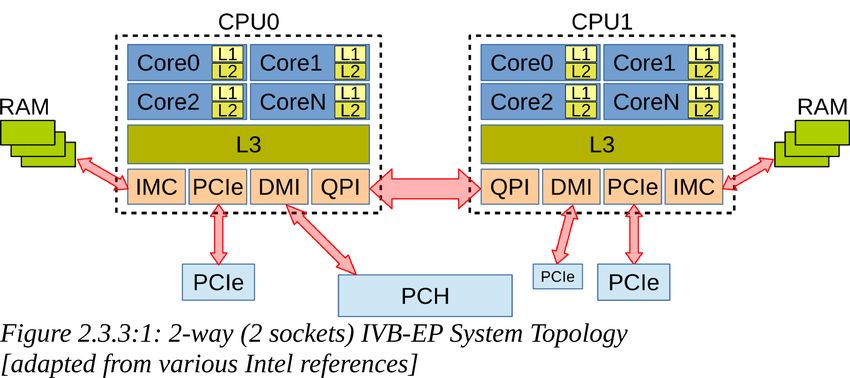
Abstract. This thesis aims to explore feasible methods to profile, from the
energy efficiency point of view, scientific applications by means of the
performance counters and the model-specific registers provided by Intel family
microprocessors. The Aurora HPC system[1] used as testbed was made
available by courtesy of CO.S.IN.T.[2], and it belongs to the same family of
machines that enabled the Eurora[3] cluster hosted at Cineca[4] to reach the 1st
rank in the 2013 Green500[5]. Retrieving power consumption information
through NVIDIA accelerators and external monitoring and management devices
on such platform is explored too.

Keywords: application-level energy profiling, energy efficiency, RAPL,
top-down characterization, performance counters, HPL, BLAS comparison,
HPCG
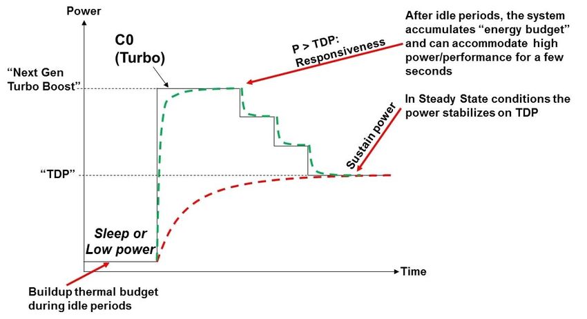
Table of Contents
1. Introduction.......................................................................................................1
   1.1. The energy problem in HPC...............................................................................1
   1.2. Motivation and approach....................................................................................3
2. Testbed..............................................................................................................5
   2.1. Hardware............................................................................................................ 5
   2.2. Software.............................................................................................................7
       2.2.1. General overview....................................................................................................7
       2.2.2. Power management and acquisition software.........................................................8
       2.2.3. Benchmarks...........................................................................................................11
       2.2.4. BLAS libraries......................................................................................................12
   2.3. Technology.......................................................................................................14
       2.3.1. Frequency scaling.................................................................................................14
       2.3.2. Hardware performance counters...........................................................................16
       2.3.3. RAPL....................................................................................................................18
       2.3.4. Top-down characterization - TMAM....................................................................20
       2.3.5. Tools......................................................................................................................22
3. Results.............................................................................................................23
   3.1. Energy measurement........................................................................................25
   3.2. HPL.................................................................................................................. 27
       3.2.1. Comparing BLAS implementations......................................................................28
       3.2.2. Top-down characterization....................................................................................30
       3.2.3. Performance counters............................................................................................31
       3.2.4. Frequency scaling.................................................................................................33
       3.2.5. Problem size scaling.............................................................................................34
       3.2.6. HPL + GPU...........................................................................................................35
       3.2.7. Summary of HPL investigation.............................................................................37
   3.3. HPCG............................................................................................................... 38
       3.3.1. Frequency and problem size scaling.....................................................................38
       3.3.2. Top-down characterization....................................................................................39
       3.3.3. Performance counters............................................................................................40
       3.3.4. Summary of HPCG investigation.........................................................................40
   3.4. Quantum ESPRESSO......................................................................................41
   3.5. LAMMPS.........................................................................................................43
   3.6. Comparison......................................................................................................47
       3.6.1. Energy efficiency and frequency scaling..............................................................47
       3.6.2. Top-down characterization....................................................................................48
       3.6.3. Performance counters............................................................................................49
4. Conclusions.....................................................................................................50
   4.1. Future Perspectives..........................................................................................51
5. Acknowledgments...........................................................................................53
6. Bibliography...................................................................................................54
7. Appendices......................................................................................................58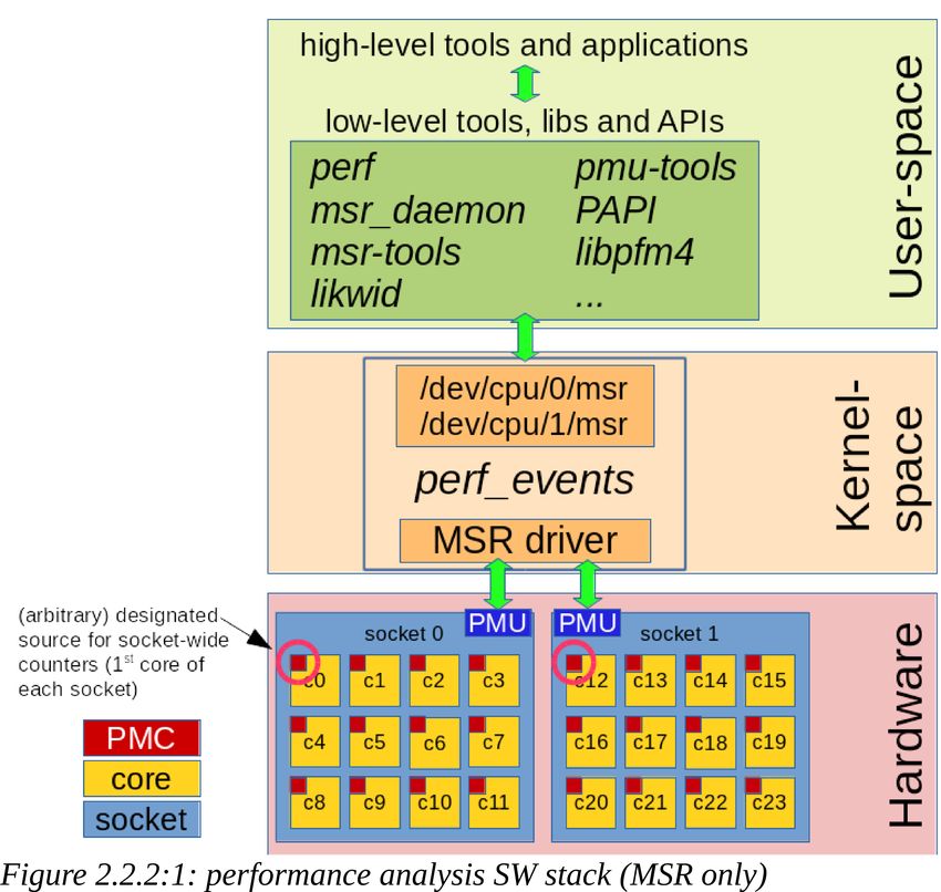
Appendix A. List of Acronyms...........................................................................58
Appendix B. TMAM formulas and performance events....................................60
Appendix C. FLOPS from performance counters...............................................61
Appendix D. Unused metrics..............................................................................62
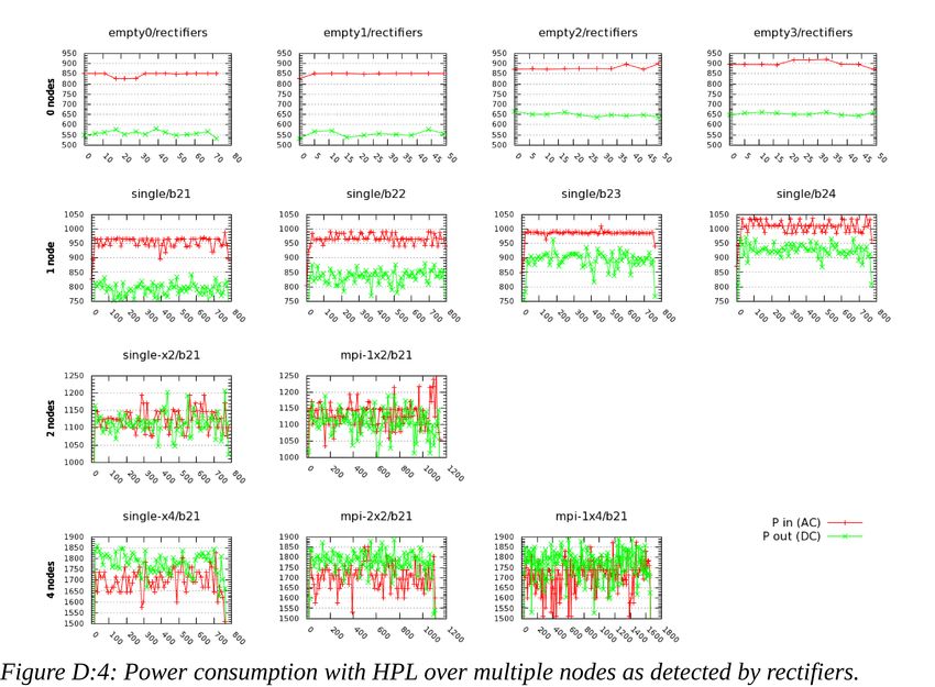
Appendix D.1. Power rectifiers................................................................................62
Appendix D.1.1. Power consumption detected by the power rectifiers..........................62
Appendix D.1.2. Detecting network devices power consumption using the rectifiers...64
Appendix D.2. Idle power consumption of the system.............................................67
Appendix D.3. msr-statd (omitted) metrics..............................................................69
Appendix E. Additional plots..............................................................................70
Appendix E.1. HPL: power consumption by CPU sub-systems...............................70
Appendix E.2. HPL: problem size scaling...............................................................72
Appendix E.2.1. BLAS comparison...............................................................................72
Appendix E.2.2. Top-down characterization...................................................................73
Appendix E.2.3. Performance counters..........................................................................74
Appendix E.3. HPL: problem size and frequency scaling........................................75
Appendix E.3.1. ATLAS.................................................................................................75
Appendix E.3.2. MKL....................................................................................................76
Appendix E.3.3. OpenBLAS..........................................................................................77
Appendix E.3.4. Netlib...................................................................................................78
Appendix E.4. HPCG: problem size and frequency scaling.....................................79
Appendix F. Playing with performance counters................................................81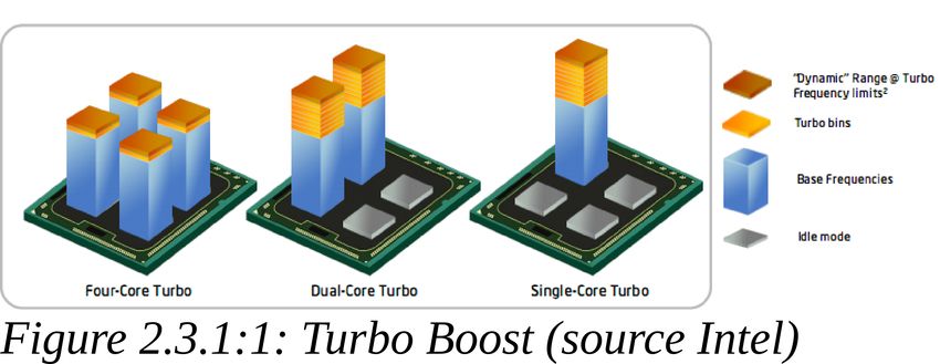
1. Introduction
In this section, the main concepts and the motivation behind this work will be introduced.

1.1. The energy problem in HPC
Energy-consumption is one of the main limiting factors for the development of High Performance
Computing (HPC1) systems into the so-called "exascale" computing, which consists of systems
capable of at least one exaFLOPS. Indeed, the Top500 project[6], which ranks and details the 500
most powerful computer systems in the world, already reports power consumption in the order of
the thousands kilo Watts for systems with “few” petaFLOPS of computational power. As of
2015/11, 212 supercomputers declare a total power of over 1 MW, 3 of which over 10 MW:
"Tianhe-2"[7], the supercomputer currently ranked at the top of the list with 34 PFLOPS, requires
17.8 MW, and "QUARTETTO"[8], a cluster ranked “only” 67th with 1 PFLOPS, requires even
more, 19.4 MW. Following this trend, an exascale supercomputer built with the technology
available today would demand a power budget in the order of 500 MW, sustainable only with a
dedicated power plant. For this reason feasible exascale supercomputers will have to fulfill the
20 MW power budget.[9] Reaching this target will require an energy-efficiency of 50 GFLOPS/W,
one order of magnitude higher than today's greenest supercomputer. In fact, the Green500[10] list,
which sorts the Top500 by energy-efficiency, ranks Tianhe-2 only 90 th and QUARTETTO 499th. The
greenest computer as of 2015/11, “Shoubu”[11], is capable to deliver 7 GFLOPS/W (ranked 135th in
the Top500), which would still need 143 MW if scaled up to exascale.
Several power management strategies can increase dynamically the final energy-efficiency of a
supercomputer by keeping the power consumption under control or by assessing the energy
efficiency online. Practical examples can span from the power capping features of a job scheduler,
to the (unattended) energy profiling of an application, tasks taken into exam with the project hereby
presented.

In addition, due to energy cost and availability, power consumption of data centers is facing as one
of the rising problems, thus energy efficiency is rapidly becoming a hot topic, especially moving
towards exascale systems. "Green" computing is now often coupled to high-performance
computing, introducing a new concept of "high-efficiency" computing, especially due to the fact
that the total cost of ownership (TCO) of a HPC infrastructure is largely impacted by the power
consumption during its life cycle.

This growing interest in energy efficiency is leading to new approaches to HPC as well as new
hardware requirements. Sysadmins, engineers, decision makers (and eventually users) are becoming
aware of the energy problem. There's a growing need for energy-aware resource management and
scheduling, in order to implement and enforce power capping constraints. Doing this, though,
requires probes and tools for monitoring the power consumption of a system and change the power
consumption of the hardware at run-time. To accomplish this, hardware/software sensors report
near-real-time power consumption. The software interfaces for accessing this information at
run-time are rapidly evolving and more often integrated in high-end infrastructures.
1   Many acronyms will be used throughout this document. Their explanation and expansion can be found in Appendix A.

1.1.The energy problem in HPC                                                                                          1
At the monitoring level, novel concepts are emerging to increase the final user awareness on the
energy efficiency. Energy-to-solution can be used to account the energy dissipated by the execution
of the user code while energy profiling of the application provides more details about the "cost in
energy" of running a specific code on a specific machine, and using a specific library.

At the power management level, several methods can be taken into account in order to reduce the
power consumption of HPC resources by adapting their performance level to the workload demand.
Power wasted by idle resources can be reduced by mean of software power management policy,
which will automatically put the idle resource into power saving modes (sleep, standby, power-off),
and will power on/wake up the nodes when new workload is available. PDU power off can be used
to further reduce the total power consumption.
Some hardware capabilities can be exploited too, for instance the Advanced Configuration and
Power Interface (ACPI) defines sleeping states (S-states), power states (C-states) and performance
states (P-states, for instance by means of Dynamic Voltage and Frequency Scaling (DVFS), Turbo
Boost technology, RFTS mechanisms and power/clock gating) in order to dynamically configure
and monitor the power consumption. All these features, which are implemented at hardware level
by the CPUs, can be enabled by compliant motherboard's BIOS and exposed as a control knob to
the operating system for run-time power-optimization.
While dynamic power management approaches, which trade-off performance for energy efficiency,
may affect the final user QoS on the supercomputer infrastructure, emerging power capping policies
[12] allows to constraint the total power consumption of the supercomputer by admitting only the
jobs which fulfill a required power budget. A run-time-enforced reduced power budget saves energy
by avoiding cooling over-provisioning. In addition by selecting the highest performance-per-watt
resources first the overall energy-efficiency can be improved.
All the above strategies are now granting a lot of attentions, and a significant effort from the HPC
industry and research community is focused on the development of energy-aware resource
management systems and schedulers.

All these techniques, to be effective, require run-time access to the system and power consumption
status. Recent generations of microprocessors introduced specific registers that allow to measure the
power consumption of different sub-systems (logical and physical areas) of the CPU with fine
granularity. For the Intel family of processors, these metrics can be obtained accessing specific
hardware counters through the Model-Specific Register (MSR) interface, in particular the so-called
Running Average Power Limit (RAPL), which allows to monitor, control, and get notifications on
System-on-Chip (SoC) power consumption (platform level power capping, monitoring and thermal
management). RAPL is not an analog power meter, but rather estimates current energy usage based
on a model driven by hardware performance counters, temperature and leakage models, and makes
this information accessible through a set of counters[13].

In addition, large infrastructures can count on several sensors and devices, for instance local
machine hardware sensors, power distribution units (PDU), power grid counters, external hardware
dependent probes and sensors. High-end machines offers out-of-band management and monitoring
capabilities (independently of the host system's CPU, firmware, OS), through the so-called
Intelligent Platform Management Interface (IPMI), which allows the monitoring of system
temperatures, voltages, fans, and power supplies.

1.1.The energy problem in HPC                                                                      2
Other external devices can be instead accessed via various standard network-based protocols, like
the Simple Network Management Protocol (SNMP), or proprietary protocols and connections.

Additional local hardware probes and sensors interfaced to the motherboard (depending on the
vendor and models) can be queried using lm-sensors (Linux monitoring sensors), which provides
tools and drivers for monitoring temperatures, voltage, humidity and fans. The fam15h_power driver,
for instance, permits to read the CPU registers providing power information of AMD Family 15h
processors, similarly to what RAPL does for Intel microprocessors, although without the same level
of granularity.

1.2. Motivation and approach

Power capping capabilities, energy-based policies and energy-aware scheduling, all require some
insights concerning the power consumption of the system. Choices concerning the evolution of such
systems must be based on the ability to estimate the power consumption of a specific job depending
on the resources requested and the kind of task or calculation that will be performed. CPU-bound
application will draw more power from the CPU, and probably less from memory and storage.
Memory-bound applications will demand more activity from memory and storage than from the
CPU, thus moving the larger power consumption to other sub-systems, while the CPU will be
probably idling most of the time. Real world applications are often a combination of both, and
identifying which part will prevail may be an indication of what the power consumption could be.
Therefore, the capability of collecting application-based energy profiles and monitoring the power
consumption of the entire system, will allow an energy-aware scheduler to predict the trend based
on the applications that are queued for execution, and hence schedule the jobs in a way that allow to
respect imposed power capping constraints.

The purpose of the first phase of this project was to determine an energetic profile for some
well-known scientific applications, by identifying, in particular, the power consumption relative to
some specific routines or hardware activities. Furthermore, this profiling included the comparison
between different BLAS implementations, as supplied by widely used mathematical libraries, for
the same application, thus highlighting how different implementations of the same family of
routines can affect the power consumption in order to solve the very same problem.

Most of the tests in this phase involved the High Performance Linpack (HPL) and the High
Performance Conjugate Gradient (HPCG) benchmarks. Besides being well-known applications,
used to characterize and rank the clusters of the Top500, these tools were chosen because the first is
a CPU-bound application, while the second is memory-bound, difference that allowed to perform a
study of the trade-off between energy consumption and performance by changing the frequency of
the CPUs (DVFS).
HPL was compiled in several versions making possible to compare the performance delivered by
various BLAS implementations, in particular Netlib[14], ATLAS[15], OpenBLAS[16],
PLASMA[17], Intel MKL[18].

1.2.Motivation and approach                                                                         3
In the second phase of this project, a couple of real-world scientific applications was tested,
Quantum ESPRESSO[19] and LAMMPS[20]. All the methods used to analyze the previous
benchmarks were then used on these applications. A lot of efforts was dedicated to the analysis of
the performance counters and the top-down characterization, issues explained in details in section
2.3 and throughout section 3.

With the exception of Intel's MKL, only Free and Open-Source Software (FOSS) was employed in
this study. NVidia's CUDA accelerated Linpack was also used in this research, even though not
strictly open.

The outline of this work is as follows: in section 2 the testbed will be explained both at hardware
and software level, including the technological issues and solutions explored and eventually
adopted, as well as the way the benchmarks were chosen. In section 3, the results obtained will be
exposed and discussed in details, for each type of analysis performed throughout this work. Finally,
section 4 is devoted to the conclusions and the future perspectives that this research stimulated.
A rich set of appendices complete the work. Some specific details concerning analysis methods are
reported in Appendix B. and Appendix C., while the results of exploratory testing are presented in
Appendix D. Finally, many of the plots produced and cited in this document have been collected in
Appendix E. and Appendix F.

1.2.Motivation and approach                                                                       4
2. Testbed

In this section, the development platform will be introduced and detailed. In particular, the
hardware, the software and the technological peculiarities of the approach are explained in
dedicated subsections.

2.1. Hardware

The basic requirements to perform this work were:
    • super-user's privileges;
    • dedicated master node + at least 2 computing nodes;
    • Intel family processors supporting RAPL.
The infrastructure in production at COSINT (Amaro, UD, Italy) was able to fulfill all the
requirements, and offered even more. The available platform, an Aurora[1] system developed by
Eurotech S.p.A., was an ideal platform for this kind of analysis since it belongs to the same
architecture that reached the 1st position in the 2013 Green500[5], the “greenest” platform, with
3.2 GFLOPS/W.

Full control over a virtual machine (VM), used for testing SLURM[21], and a computing node was
initially granted full-time for the whole period covered by this project. Few more computing nodes
were made available occasionally for scaling tests, and external monitoring devices were made
accessible too.
The Aurora computing nodes under exam are equipped with 2 Intel Xeon Ivy Bridge processors
with 12 cores each at 2.7 GHz, 64 GB of RAM, and 2 NVidia K20 GPUs.

In detail, the tests on this platform involved the following machines:
    • 1x masternode / access node;
    • 1x AURORA chassis with 6 blade (no accelerators);
    • 1x AURORA chassis with 4 blade (2x NVIDIA GPU K20 on each blade);
    • 10x blades with 2x 12-cores CPU Intel Ivy Bridge @2.7 GHz, and 64 GB of RAM;
    • 1x virtual machine installed and configured as SLURM server;
    • 2x blades configured as SLURM compute nodes.

The chassis used for most of the tests may be reported in plots and tables as "chassis 2".
The blade used for most of the tests is "b21" ('b'lade node, chassis #2, blade #1).

Unfortunately, the original design of the Aurora platform, developed with the clear intent of
providing an innovative and energy-friendly system (successfully), presents some side effects too.
Due to the peculiar experimental nature of the platform (in between a technology demonstration and
a production-ready architecture), some tools and sensors often available and used on mass-produced

2.1.Hardware                                                                                    5
high-end platforms are not available or just not implemented yet. For instance, the IPMI interface that manages the blades cannot be queried in order to obtain temperature and power readings, and the system does not offer any alternative interface or remotely-accessible sensor for this purpose. Nevertheless, the external power supply can be queried via SNMP and it is able to provide real-time voltage, current, and temperature readings from the monitoring sensors of its 6 power rectifiers (electrical devices that convert alternating current (AC) to direct current (DC)). Each of the 2 available chassis of blades are directly powered by 3 of these 6 rectifiers. By combining the data collected from the 3 rectifiers connected upstream, it is possible to derive the total power absorbed by all the blades of a chassis, although this value includes the chassis itself (rootcard controller, fans, ...). The granularity and precision are clearly suboptimal, but the idea was to obtain differential readings in order to exclude the background power consumption of the chassis and idling blades. In order to obtain as much data as possible for the study of the power consumption, some tests hence included the reading obtained querying these devices while the benchmarks were running on one or more nodes at the same time (while the other nodes were idling). The analysis of these readings is reported in Appendix D.1. Most of the analysis hereby presented are based upon the microprocessor and its features. The processor in use on the test platform is the Intel Xeon Ivy Bridge EP E5-2697 v2 @ 2.70 GHz[22], with 30 MB of L3 cache, in a dual-sockets server platform configuration (code-named Romley). Section 2.3 will reveal additional details concerning the features of this family of processors. The Figure 2.1:1 shows the internal topology of the processor as reported by lstopo (hwloc[23]). 2.1.Hardware 6
2.2. Software

This section provides all the details concerning the software layers of the test environment. The
needs, and the software tested, developed, and eventually adopted will be discussed.

2.2.1.General overview

The operating system used is Linux, in particular a CentOS distribution [24], version 6.5, with the
stock kernel 2.6.32-358.23.2.el6.x86_64 and default utilities. Additional packages, detailed in
sections 2.2.2 and 2.3, have been installed to perform low-level operations, like handling the power
governor, the frequency scaling, and the performance counters.

The libraries and executables were compiled using the GNU compiler version 4.8.3 [25] and
OpenMPI version 1.8.3 [26]. A license for Intel compilers and MPI was not available on the
platform used. Any difference in performance, though, was deemed irrelevant for the kind of
analysis meant to be performed on the system and on the software stack.

Even though the cluster was configured to use PBS-Pro[27] as resource manager and job scheduler, it
was not involved during most of the tests, as direct access to the computing nodes was preferred
(avoiding cpusets and other unwanted features). PBS-Pro doesn't currently support out-of-the-box
energy-based scheduling policies, power capping mechanisms and per-job energy reports.
SLURM[21], though, an open-source workload manager, is rapidly evolving in this direction, already
allowing to enable the report of per-job power consumption, and it is rapidly moving toward
implementing and providing power capping capabilities and energy-based fair-sharing too.[28][29]
A virtual machine and a couple of computing nodes were temporary dedicated to setup such
framework (SLURM 14.11.7), and some tests have been conducted to investigate its features. The
per-job energy reports, in particular, were used to compare the results obtained by the means of
other monitoring utilities.

The Eurora Monitoring Framework [30], a set of scripts and utilities developed by Micrel
Lab[31]/UNIBO[32]/CINECA[4] and used for similar analysis on the Eurora cluster[3], was used in
order to access the hardware performance counters and record the power consumption of a node
during the run of the application under exam.
In the setup phase, the framework was adapted and improved. Some utilities, in particular the one
which acquires the MSR/RAPL counters, called msr-statd, and the one devoted to filter the data
(msr-filter), have been modified in order to work on the COSINT cluster, and virtually, anywhere
else too. In particular, these utilities have been interfaced to hwloc and numactl[33] in order to
automatically detect the hardware configuration at runtime (number of sockets, number of cores,
core-to-socket map), and many command-line options have been added in order to modify at will all
the vital parameters, hardcoded at compile-time in the original version.
The overhead of this utility was considered negligible as its CPU-time was measured in
1.2 milliseconds for each reading performed at regular intervals of 10 or 5 seconds. Should be noted
that, due to the size of the registers and the frequency these registers are updated by the CPU, the
interval must be kept reasonably short (
reported by SLURM and msr-statd resulted to be compatible and reliable, likwid-powermeter, though,
reported values that wasn't possible to associate clearly to specific resources utilization. By using
LIKWID versions 3.1.3 and 4.0.0, the values reported were not even compatible with each other. After
these results, LIKWID was not used for further testing. Should be noted, though, that at the time of
this writing, the current git version of LIKWID (as retrieved the 2015/10/16) reports values compatible
with the readings obtained with SLURM and the msr-statd utility.
At the end of this comparison, the software developed by Micrel Lab was chosen as it suited best all
the requirements, as it is stand-alone, out-of-band (no instrumentation of the tested code is needed),
flexible, easy to use and to adapt.

Performance monitoring events represent a powerful tool for the profiling and improvement of the
performance of an application. Some of these performance events permit to understand whether an
application is memory-bound or CPU-bound, or maybe bound to other components such as the
GPU. This allows to identify where the application is bottlenecked and possibly indicate how to
improve it.
A preliminary phase was devoted to study the available Linux utilities, libraries and APIs for the
management and monitoring of system performance and energy consumption, as well as
programming techniques for low-level access to CPU performance counters and registers.
The various tools and techniques that have been used to retrieve and analyze such kind of
information will be illustrated and discussed throughout this document.

Several ad-hoc scripts and utilities were developed in order to collect other pieces of information
and useful data for the analysis. Some of these scripts were used to access, for instance, the power
rectifiers via SNMP, while many others were just wrapper scripts for “perf” and other utilities
(msr-statd, cpufreq, ...), in order to automate the simulations by varying many of the parameters
(core frequency, problem size, performance counters, ...). Many others were written and used to
collect, parse and filter the huge amount and variety of data obtained. All these tools have been
collected in a git repository and will be soon published as open-source software.

2.2.2.Power management and acquisition software
Various software was investigated, tested and used in order to acquire and collect the information
needed, as well as for managing the environment. This section briefly reviews them, giving also
some usage examples.

As mentioned in the previous section, the software developed by Micrel Lab/UNIBO on their study
of the Eurora cluster, was modified and widely used to obtain RAPL power readings from the CPU.
msr-statd is a MSR/RAPL acquisition software written in C, linked to hwloc and numactl, that
requires super-user's privileges in order to access the MSR kernel module interface (/dev/cpu/*/msr).
Usage example:
       msr-statd --hwloc --background --path $PWD --prefix xhpl.openblas --interval 5 --truncate
       msr-filter --input xhpl.openblas.msr.log > xhpl.openblas.msr.log.report
       msr-compact.pl < xhpl.openblas.msr.log.report > xhpl.openblas.msr.log.summary

Concerning GPU power readings, a python script named gpu-statd (as well part of the Micrel Lab's
Eurora Monitoring framework) interfaced to the NVidia Management Library (NVML)[35]
provided power consumption and load of the GPUs. Similar readings, even though with a far larger
overhead, can be obtained by using the utility nvidia-smi[36].
Usage example:
       gpu-statd start --path $PWD --prefix xhpl.nvidia --ts 5
       gpu-filter.py --input xhpl.nvidia.gpu.log --gpus 2 > xhpl.nvidia.gpu.log.report

2.2.2.Power management and acquisition software                                                      8
Additional power consumption information was supposed to be collected by accessing the rectifiers
and the power management of the Aurora blades. SNMP utils[37] and IPMI tools[38] were used in
order to access the external power rectifiers and the IPMI management interface of the blades.
Some ad-hoc utilities were written in order to setup and poll the power supply and get readings at
regular intervals.
Usage example:
ipmitool -H sp-b21 -U foo -P bar power status
ipmiwrap.sh b21 sensor list
snmpwalk -mALL -v2c -cfoobar pdu .1.3.6.1.4.1.10520.2.1.5.6.1.8
snmpbulkwalk -mALL -v2c -cfoobar pdu .1.3.6.1.4.1.10520.2.1.5.6.1.10
pductl -f status all
pductl -f pout 2
cpufreq-utils[39], a user-space utility provide by the kernel tools, was used to query and modify the
frequency scaling governor and the CPU frequency, even though it was wrapped by a script to
simplify and modularize the utilities used.
(setting frequency and governor requires super-user's privileges).
cpufreq-info
seq 0 23 | xargs -t -i cpufreq-set -r -c {} -g userspace
seq 0 23 | xargs -t -i cpufreq-set -r -c {} -f 2700000
Direct access to sysfs[40] was exploited too for the same tasks. Sysfs is a virtual filesystem on
Linux, which provides user-space access to kernel objects, like data structures and their attributes. It
is possible to read and write various flags, which will be applied by the kernel to the proper
sub-system or device.
(setting frequency and governor requires super-user's privileges).
Usage example:
read and set scaling governor:
grep . /sys/devices/system/cpu/cpu0/cpufreq/scaling_available_governors
grep . /sys/devices/system/cpu/cpu*/cpufreq/scaling_governor | sort -tu -k3n,3
echo userspace | tee /sys/devices/system/cpu/cpu*/cpufreq/scaling_governor
read and set frequency:
grep . /sys/devices/system/cpu/cpu0/cpufreq/scaling_available_frequencies
grep . /sys/devices/system/cpu/cpu*/cpufreq/scaling_cur_freq | sort -tu -k3n,3
echo 2700000 | tee /sys/devices/system/cpu/cpu*/cpufreq/scaling_cur_freq
Beside the Eurora framework, SLURM energy plugins (acct_gather_energy) and utilities provided by
LIKWID (likwid-powermeter and likwid-perfctr) were tested to evaluate their capabilities of reporting
energy consumption of a job/process, A comparison was performed to verify the power readings
obtained and their reliability, in order to figure out the most complete and flexible alternative
(msr-statd was eventually chosen).
(may require super-user's privileges for some metrics)
Usage example:
likwid-powermeter
likwid-perfctr -f -c 0-23 -C 0-23 -g ENERGY mpirun --np 24 xhpl
likwid-perfctr -f -c 1 -C 1 -g BRANCH /bin/ls
Linux Perf[41] was extensively used in order to collect the performance counters, needed also to
perform the top-down characterization. Perf is a native Linux utility that interfaces its kernel-space
layer (perf_events) to the user-space, allowing to access, read and collect the performance counters
during the run time of a process. Perf_events interacts with the model-specific registers (MSR) and
the performance monitoring unit (PMU) of the CPUs through the msr kernel module. The data
collected can be post-processed in order to perform a deeper analysis and extract derived metrics,
obtaining low-level runtime information about the software under exam, its performance, and its
bottlenecks.
(may require super-user's privileges for some metrics)
Usage example:
perf stat sleep 1
perf stat -e branch-instructions,branch-misses /bin/ls
2.2.2.Power management and acquisition software 9perf stat -o ./perf.log -x, -e r03c,r19c,r2c2,r10e,r30d /bin/ls
perf stat -a -x, -o ./perf.log \
-e cpu/config=0x003C,name=CPU_CLOCK_UNHALTED_THREAD_P/ \
-e cpu/config=0x019C,name=IDQ_UOPS_NOT_DELIVERED_CORE/ \
-e cpu/config=0x02C2,name=UOPS_RETIRED_RETIRE_SLOTS/ \
-e cpu/config=0x010E,name=UOPS_ISSUED_ANY/ \
-e cpu/config=0x030D,name=INT_MISC_RECOVERY_CYCLES/ \
mpirun --np 24 xhpl
Finally, a huge number of ad-hoc scripts, filters, parsers and wrappers to run the benchmarks and
collect and analyze the data were written in bash, awk, sed, perl, python, C, gnuplot[42].
2.2.2.Power management and acquisition software 102.2.3.Benchmarks Four different applications were used in this work: two HPC standard benchmarks and two scientific applications in materials science. All the four packages are well-known in their respective scientific domain. High Performance Linpack benchmark and the High Performance Conjugate Gradient benchmark. have been used in the first phase to investigate and calibrate the profiling methods. High Performance Linpack (HPL) is a portable implementation of the High Performance Computing Linpack Benchmark widely used to benchmark and rank supercomputers for the Top500 list. HPL is CPU and memory intensive with non-ignorable communication. HPL generates a linear system of equations of order n and solves it using LU decomposition with partial row pivoting. It requires installed implementations of MPI and makes use of the Basic Linear Algebra Subprograms (BLAS) libraries for performing basic vector and matrix operations. The HPL package provides a testing and timing program to quantify the accuracy of the obtained solution as well as the time it took to compute it. The best performance achievable by this software on a system depends on a large variety of factors. The algorithm is scalable in the sense that its parallel efficiency is maintained constant with respect to the per-processor memory usage.[43] The second benchmark tested is HPCG, the High Performance Conjugate Gradient, a benchmark designed to validate the performance of a supercomputer by simulating an utilization of the resources closer to the real-world applications, often bound to frequent and sparse memory accesses and inter-node communication more than CPU dense computation. High Performance Conjugate Gradient (HPCG) is a self-contained benchmark that generates and solves a synthetic 3D sparse linear system using a local symmetric Gauss-Seidel preconditioned conjugate gradient method. The HPCG Benchmark project is an effort to create a more relevant metric for ranking HPC systems than the HPL benchmark. Reference implementation is written in C++ with MPI and OpenMP support.[44] Jack Dongarra, presenting the benchmark[45][46], talks about a “Performance shock”. The performance observed with HPCG can be even less than 1% of the peak performance of a system, far away from those obtained with HPL based mainly on the computing power of the CPU. The fact that the algorithm is known, the applications are reliable, the input finely configurable, and both provide performance and timing, made of these tools the perfect samples to profile and later use as a reference for comparison. Beside these reasons, HPL is a CPU-bound application, while HPCG is memory-bound. This simple and basic difference permits to figure out how much being dense (or not) in the CPU influences the power consumption of an application. HPL was tested by linking various BLAS implementations, and for each of them, various performance counters were collected and later used for further analysis. The power consumption of HPL was also monitored changing frequency scaling governor and forcing different CPU frequencies for each run. Another test was performed to investigate the hybrid CPU+GPU implementation (optimized and precompiled by NVidia), in order to verify the impact in terms of energy efficiency of moving the computation from the CPU to the GPU and scaling down the CPU frequency. 2.2.3.Benchmarks 11
The tests performed on HPCG include the power consumption by varying CPU frequency, problem
size scaling test, as well as performance counters analysis and top-down characterization.

These two benchmarks were largely investigated in order to obtain reliable basis to study additional
applications, whose behavior could be unknown, but likely residing within the “extremes”
represented by HPL and HPCG.

The next stage was dedicated to the analysis of two scientific applications commonly used in HPC,
taken as real-world examples of actual calculations performed on the cluster under exam: Quantum
ESPRESSO and LAMMPS.

Quantum ESPRESSO is a software suite for ab-initio quantum chemistry methods of
electronic-structure calculation and materials modeling. It is based on Density Functional Theory,
plane wave basis sets, and pseudopotentials. The core plane wave DFT functions of QE are
provided by the PWscf (Plane-Wave Self-Consistent Field) component, a set of programs for
electronic structure calculations within density functional theory and density functional perturbation
theory, using plane wave basis sets and pseudopotentials.[19]
The data set used for Quantum ESPRESSO ( pw.x in particular) is a scaled down input taken from a
real simulation performed by a user of the cluster. In this test a Palladium surface is modeled, using
a slab geometry. Most of the computational time is therefore spent in linear algebra operations such
as matrix-vector multiplications, as well as in fast Fourier transforms.

LAMMPS is a classical molecular dynamics code. LAMMPS has potentials for solid-state materials
(metals, semiconductors) and soft matter (biomolecules, polymers) and coarse-grained or
mesoscopic systems. It can be used to model atoms or, more generically, as a parallel particle
simulator at the atomic, meso, or continuum scale. LAMMPS runs on single processors or in
parallel using message-passing techniques and a spatial-decomposition of the simulation domain.
The code is designed to be easy to modify or extend with new functionality.[20]
The standard Lennard-Jones liquid benchmark, provided with the LAMMPS, was used to profile
the application. The input was tuned and scaled up to 70M atoms to make the runtime close to
10 minutes.

2.2.4.BLAS libraries

There are many BLAS implementations available on the market, and each implementation deliver
different level of performance. If using a different algorithm to solve the same problem leads to
difference performance, it means also that its implementation is able to exploit better (or worse) the
underlying hardware. As a consequence, the power consumption, and therefore the energy
efficiency, must be impacted too by this different distribution of the resources' utilization.
This study aimed to identify such difference.

This evaluation included the reference BLAS from Netlib, the automatically tuned implementation,
ATLAS, the proprietary and closed-source Intel MKL version, and the OpenBLAS
highly-optimized free and open-source implementation. The compilation was performed using gcc
compiler and standard optimization flags have been applied. No further tune was done at
compilation phase.

2.2.4.BLAS libraries                                                                               12
PLASMA[17] was also tested, but it relies on a 3 rd party BLAS library, and it can be compiled and
linked against any of the aforementioned BLAS implementations. Beside providing its own
implementation of many BLAS and LAPACK routines, PLASMA acts simply as a wrapper for
many others (in some cases still optimizing their access and utilization). In this case, though, it
turned out that the performance achieved using PLASMA was the very same achieved by the
underlying BLAS library it was linked to, hence the BLAS routines invoked by HPL were just
passed-through. PLASMA was therefore excluded from further analysis.

2.2.4.BLAS libraries                                                                            13
2.3. Technology

This section provides some technical details concerning the technology surrounding the power
management of the microprocessor, the hardware counters and the performance events used and
discussed in this work. This section reports also the challenges and difficulties in accessing and
interpreting low-level data and the issues faced during the tests and the analysis phase.

2.3.1.Frequency scaling

Microprocessors have seen a continuous evolution during the years, racing to reach higher clock
frequencies. The frequency increment, though, led as well to higher power consumption and
dissipation. Various solutions have been adopted in order to reduce these factors while maintaining
the performance. Aggressive power saving policies have been implemented in order to reduce the
power consumption when a resource is not in use or when the highest computing power is not
required.

The Advanced Configuration and Power Interface (ACPI) defines sleeping states (S-states), power
states (C-states) and performance states (P-states) in order to dynamically configure and monitor the
power consumption. All these features are implemented at hardware level by the microprocessors
and configurable by compliant motherboard's BIOS and, dynamically, at runtime by the operating
system.

Some of these solutions involved methods like the Dynamic Voltage and Frequency Scaling
(DVFS), Run Fast Then Stop (RFTS) mechanisms and power/clock gating. Intel processors, in
particular, supports Enhanced Intel SpeedStep (EIST) and Turbo Boost technologies, by means of
voltage and frequency scaling, internal power capping mechanisms and deep sleep states.

Intel Turbo Boost Technology is a feature that allows the processor to opportunistically and
automatically run faster than its rated operating frequency if it is operating below power,
temperature, and current limits. The result is increased performance.
The processor's rated frequency assumes that all execution cores are running an application at the
thermal design power (TDP). However, under typical operation, not all cores are active. Therefore
most applications are consuming less than the TDP at the rated frequency. To take advantage of the
available TDP headroom, the active cores can increase their operating frequency.
To determine the highest performance frequency amongst active cores, the processor takes the
following into consideration:
• The number of cores operating in the C0 state.
• The estimated current consumption.
• The estimated power consumption.
• The die temperature.
Any of these factors can affect the maximum frequency for a given workload. If the power, current,
or thermal limit is reached, the processor will automatically reduce the frequency to stay with its
TDP limit.[47]

DVFS is a technique that allows to reduce the power consumption by acting on the frequency at
which the CPU is clocked, or its voltage, or both (typically). Lowering the clock frequency, though,
usually increases the time-to-solution or walltime (or runtime) of an application. This work aims to
verify the influence of this fact on CPU-bound, memory-bound and real-life scientific applications.

2.3.1.Frequency scaling                                                                           14
CPU frequency scaling enables the operating system to scale the CPU frequency up or down in
order to save power. CPU frequencies can be scaled automatically depending on the system load, in
response to ACPI events, or manually by user-space programs.

The Dynamic CPU frequency scaling infrastructure implemented in the Linux kernel is called
CPUfreq[48]. CPUfreq is demanded to enforce specific frequency scaling policies, which consist of
(configurable) frequency limits (min,max) and CPUfreq governor to be used (power schemes for the
CPU). Available governors are:
powersave: sets the CPU statically to the lowest frequency within the borders of scaling_min_freq
   and scaling_max_freq (/sys/devices/system/cpu/cpu*/cpufreq/scaling_{min,max}_freq )
performance: sets the CPU statically to the highest frequency within the borders of scaling_min_freq
   and scaling_max_freq.
ondemand: dynamically sets the CPU depending on the current usage. Sampling rate (how often the
   kernel must look at the CPU usage and make decisions on what to do about the frequency) and
   threshold (average CPU usage between the samplings needed for the kernel to make a decision
   on whether it should increase the frequency, e.g.: average usage > 95%, CPU frequency needs to
   be increased) can be defined.
conservative: like the "ondemand" governor. It differs in behavior in that it gracefully increases and
   decreases the CPU speed rather than jumping to max speed the moment there is any load on the
   CPU. Available parameters are similar to "ondemand".
userspace: allows the (super)user to set the CPU to a specific frequency by making a sysfs file
   "scaling_setspeed" available in the CPU-device directory.
    (/sys/devices/system/cpu/cpu*/cpufreq/scaling_setspeed )

The combination of the running kernel (2.6.32-358.23.2.el6.x86_64) and the IVB-EP processor in
use on the test platform allows to select the governors ondemand, userspace or performance
(/sys/devices/system/cpu/cpu9/cpufreq/scaling_available_governors ).

The frequencies that can be selected using the “userspace” governor are (in kHz): 2701000
(Turbo Boost), 2700000 (nominal frequency), 2400000, 2200000, 2000000, 1800000 1600000,
1400000, 1200000 (/sys/devices/system/cpu/cpu*/cpufreq/scaling_available_frequencies ).

At hardware-level, the frequency is controlled by the processor itself and the P-states exposed to
software are related to performance levels. Even if the scaling driver selects a single P-state the
actual frequency the processor will run at is selected by the processor itself. In order to reduce
energy costs, the processor may also shift one (or more) core and memory into lower power states
(higher C-state) when idle, despite a P-state was selected by the OS. C-states available on the
IVB-EP are C0 (active), C1 (halt), C3 (deep-sleep), C6 (deep power down). This phenomenon is
observed in Appendix D.2.

2.3.1.Frequency scaling                                                                            15
2.3.2.Hardware performance counters
Most modern microprocessors provide hardware counters that monitor and report the count of
hardware-related events concerning the CPU and its activity, including information like the elapsed
clock ticks, instructions issued and retired, cache hits/misses, memory accesses and I/O read/write
operations, which allow to obtain various derived metrics.
These hardware counters, called Performance Monitoring Counters (PMC), can be accessed using
low-level calls to specific Configuration Space Registers (CSR), and can be used for the monitoring
of the performance of the system, profiling of applications and their tuning. Various types of
performance counter are implemented, covering different performance interests. Some counters can
provide information regarding each single core of the CPU, some provide socket-wide information.
“Socket” and “package” are sometimes used interchangeably, but relate to the same concept:
everything available on the processor die. Other distinctions will be discussed in the following
sections.
The IVB-EP processors support the following configuration register types:
• PCI Configuration Space Registers (CSR): chipset specific registers that are located at PCI
defined address space.
• Machine Specific Registers (MSR), accessible by specific read and write instructions (rdmsr,
wrmsr) accessible by OS ring 0 (the kernel mode with the highest privilege) and BIOS.
• Memory-mapped I/O (MMIO) registers: accessible by OS drivers.
The followings are the counters available on IVB-EP and directly or indirectly used in this work:
- per-core counters:
• 3 fixed-purpose counters, each can measure only one specific event:
Counter name Event name
FIXC0 INSTR_RETIRED_ANY
FIXC1 CPU_CLK_UNHALTED_CORE
FIXC2 CPU_CLK_UNHALTED_REF
• 4 general-purpose counters, PMC, each can be configured to report a specific event.
• 1 thermal counter which reports the current temperature of the core.
- socket-wide counters:
• Energy counters: provide measurements of the current energy consumption through the
RAPL interface (see section 2.3.3).
Counter name Event name
PWR0 PWR_PKG_ENERGY
PWR1 PWR_PP0_ENERGY
PWR2 PWR_PP1_ENERGY (not available on IVB-EP)
PWR3 PWR_DRAM_ENERGY
• Home Agent counters (BBOXC): protocol side of memory interactions, memory
reads/writes ordering (modular ring to IMC)
• LLC-QPI fixed and general-purpose counters (SBOXFIX, SBOXC): LLC
snooping/forwarding and LLC-to-QPI related activities.
• LLC counters (CBOXC): LLC coherency engine
• UNCORE counters (UBOXFIX, UBOX): measurements of the management box in the
uncore (frequency of the uncore, physical read/write of distributed registers across physical
processor using the Message Channel, interrupts handling)
• Power control unit (PCU) fixed and general-purpose counters ( WBOXFIX, WBOX):
measurements of the power control unit (PCU) in the uncore (core/uncore power and
thermal management, socket power states)
2.3.2.Hardware performance counters 16• Memory controller fixed and general-purpose counters ( MBOXFIX, MBOXC):
DRAM related events (clock frequency, memory access, ...)
• Other Ring related counters: Ring to QPI (RBOXC), Ring to PCIe (PBOX)
• IRP box counters IBOXC
Some of the aforementioned counters can be accessed through the MSR interface, for which Linux
provide a specific driver and device, others through specific PCI or MMIO interfaces.
While per-core counters can be read from each core of the socket, socket-wide counters, like RAPL,
can be accessed only from one of the cores (any one). msr-statd, the utility used to obtain the power
consumption, was modified in order to use the PMU of the first core of each socket as source for
socket-wide RAPL counters.
The general-purpose counters can be configured to read one of the hundreds of events supported by
the processor[49]. Since there are 4 general-purpose counter available, only 4 events can be
monitored at the same time (besides the fixed counters which are always available but not
configurable).
In order to overcome this limitation, some utilities like perf, implement a multiplexing method that
allows to switch the monitored events (PMU events only). With multiplexing, an event is not
monitored continuously, but only for some repeated timed intervals, sharing the counter during the
measuring period. At the end of the run, the aggregated event count is scaled for the complete
period, thus providing an estimate of what the count could have been if it was measured for the
whole run. Hence, scaled results are not completely reliable, as some blind spots may hide spikes,
providing misleading results.
Counts reported by the fixed counters can be also obtained from equivalent configurable
performance events on the general-purpose counters. Unfortunately, though, because of many
factors, the values obtained differ, and this was one of the elements of confusion experienced during
the test phase.
Each performance event is represented by an event number and a mask. In section 3 and appendices
B and C, for all the events taken into exam, either the event name, the aliases or the hex flags (or
all) may be reported.
Unfortunately, each generation of processors, and even different variants of the same model, can
provide different counters and many different events. Sometimes new events are introduced,
sometimes are removed, sometimes not implemented, and sometimes measure something different
for each version. In the official documentation, sometimes the same metric is represented with
multiple names and not always consistently. All this, and the differences introduced in the name
spaces implemented in various monitoring and profiling software, make extremely difficult to
pinpoint the exact meaning and usage of a specific event. Moreover, different utilities use different
events claiming the same purpose. For sure, keeping such kind of software up-to-date for each new
variant of processor and new innovation require a lot of efforts, and results can be only as accurate
as the details available in the official documentation.
In order to provide a generic interface common for all the processors, Linux Perf/Kernel developers
implemented some “aliases” for common events (unfortunately not always correct across different
platforms), but kept open the possibility for a final user to specify explicitly an event to monitor.
This feature was widely used in this work.
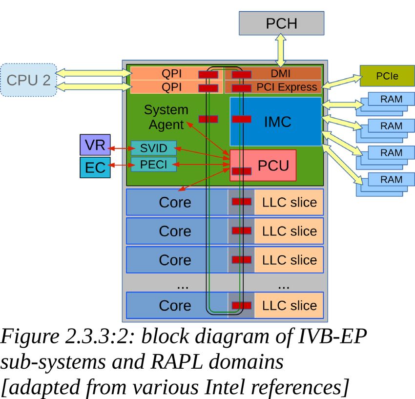
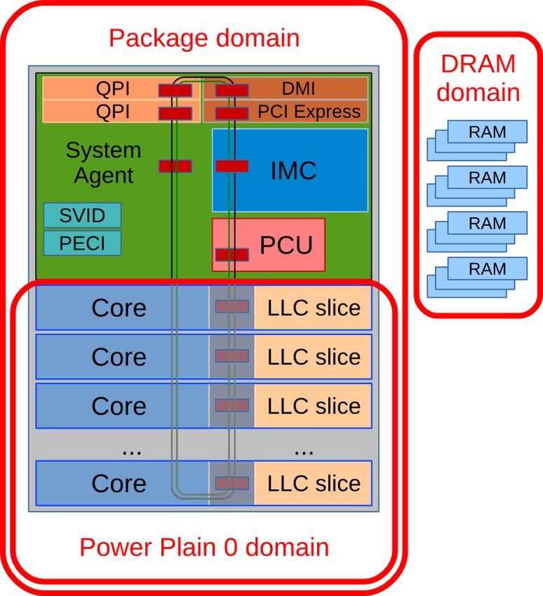
2.3.2.Hardware performance counters 172.3.3.RAPL Recent generations of Intel processors offer specific registers and counters which report, among thousands things, the power consumption of the CPU based on its main areas and functionality, like DRAM, CORE and UNCORE sub-systems. The UNCORE, called System Agent since Sandy Bridge, collects the functions of the microprocessor that are not in the CORE, but are essential for its performance. See figures 2.3.3:1 and 2.3.3:2. Depending on the family/model, the sub-systems and the functions associated to each of them may vary. According to various (sometimes fuzzy) documentation[50][51][52][47][53], on Intel Ivy Bridge EP the sub-systems are divided as following: • CORE: components of the processor involved in executing instructions, including ALU, FPU, L1, L2 and L3 cache;(*) • UNCORE or System Agent: integrated memory controller (IMC), QuickPath interconnection (QPI), power control unit (PCU), ring interconnect, misc I/O (DMI, PCI-Express, ...).(*) For desktop and mobile models, the Ivy Bridge processors may also include the Display Engine (included in the UNCORE/System Agent) and the integrated graphics processor (IGP). The Figure 2.1:1 in section 2.1 (Hardware), shows the CPU internal topology (Core, L1i, L1d, L2, L3, DRAM) as reported by lstopo (hwloc). Figure 2.3.3:1 shows the system topology. In RAPL[54], platforms are divided into domains for fine grained reports and control. A RAPL domain is a physically meaningful domain for power management. The specific RAPL domains available in a platform vary across product segments. Ivy Bridge platforms targeting server segment support the following RAPL domain hierarchy: • Power Plane 0 (PP0): all cores and L1/L2/L3 caches on the package/die/socket (CORE) • Package (PKG): processor die (PP0 + anything else on the package/die/socket (UNCORE)) • DRAM: directly-attached RAM From the above, can be derived that UNCORE=PKG-PP0. Each level of the RAPL hierarchy provides respective set of RAPL interface MSRs. (*) for the acronyms, please refer to Appendix A. 2.3.3.RAPL 18
You can also read