Presentation and discussion of the high-resolution atmosphere-land-surface-subsurface simulation dataset of the simulated Neckar catchment for the ...
←
→
Page content transcription
If your browser does not render page correctly, please read the page content below
Earth Syst. Sci. Data, 13, 4437–4464, 2021
https://doi.org/10.5194/essd-13-4437-2021
© Author(s) 2021. This work is distributed under
the Creative Commons Attribution 4.0 License.

          Presentation and discussion of the high-resolution
       atmosphere–land-surface–subsurface simulation dataset
           of the simulated Neckar catchment for the period
                              2007–2015
       Bernd Schalge1 , Gabriele Baroni2 , Barbara Haese3 , Daniel Erdal4 , Gernot Geppert5 , Pablo Saavedra1 ,
        Vincent Haefliger1 , Harry Vereecken6,7 , Sabine Attinger8,9 , Harald Kunstmann3,10 , Olaf A. Cirpka4 ,
             Felix Ament11 , Stefan Kollet6,7 , Insa Neuweiler12 , Harrie-Jan Hendricks Franssen6,7 , and
                                                   Clemens Simmer1,7
                              1 Institute       for Geosciences, University of Bonn, Bonn, Germany
                  2 Department          of Agricultural and Food Sciences, University of Bologna, Bologna, Italy
                                 3 Institute of Geography, University of Augsburg, Augsburg, Germany
                           4 Center for Applied Geoscience, University of Tübingen, Tübingen, Germany
                                    5 Department of Meteorology, University of Reading, Reading, UK
                              6 Forschungszentrum Jülich GmbH, Agrosphere (IBG-3), Jülich, Germany
        7 Centre for High-Performance Scientific Computing (HPSC-TerrSys), Geoverbund ABC/J, Jülich, Germany
                   8 Institute of Earth and Environmental Science, University of Potsdam, Potsdam, Germany
                                   9 Helmholtz-Center for Environmental Research, Leipzig, Germany
           10 Institute of Meteorology and Climate Research (IMK-IFU), Karlsruhe Institute of Technology (KIT),

                                                    Garmisch-Partenkirchen, Germany
                                11 Meteorological Institute, University of Hamburg, Hamburg, Germany
                         12 Hannover, Institut für Strömungsmechanik und Umweltphysik im Bauwesen,

                                            Leibniz Universität Hannover, Hannover, Germany
                                 Correspondence: Bernd Schalge (bschalge@uni-bonn.de)

                                Received: 6 February 2020 – Discussion started: 30 March 2020
                        Revised: 28 May 2021 – Accepted: 20 June 2021 – Published: 14 September 2021

      Abstract. Coupled numerical models, which simulate water and energy fluxes in the subsurface–land-surface–
      atmosphere system in a physically consistent way, are a prerequisite for the analysis and a better understand-
      ing of heat and matter exchange fluxes at compartmental boundaries and interdependencies of states across
      these boundaries. Complete state evolutions generated by such models may be regarded as a proxy of the real
      world, provided they are run at sufficiently high resolution and incorporate the most important processes. Such
      a simulated reality can be used to test hypotheses on the functioning of the coupled terrestrial system. Coupled
      simulation systems, however, face severe problems caused by the vastly different scales of the processes act-
      ing in and between the compartments of the terrestrial system, which also hinders comprehensive tests of their
      realism. We used the Terrestrial Systems Modeling Platform (TerrSysMP), which couples the meteorological
      Consortium for Small-scale Modeling (COSMO) model, the land-surface Community Land Model (CLM), and
      the subsurface ParFlow model, to generate a simulated catchment for a regional terrestrial system mimicking
      the Neckar catchment in southwest Germany, the virtual Neckar catchment. Simulations for this catchment are
      made for the period 2007–2015 and at a spatial resolution of 400 m for the land surface and subsurface and
      1.1 km for the atmosphere. Among a discussion of modeling challenges, the model performance is evaluated
      based on observations covering several variables of the water cycle. We find that the simulated catchment be-
      haves in many aspects quite close to observations of the real Neckar catchment, e.g., concerning atmospheric

Published by Copernicus Publications.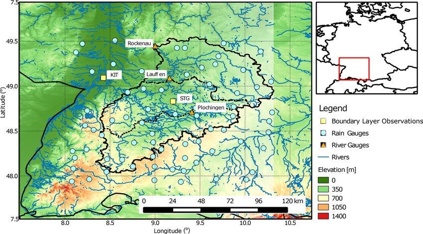
4438                                              B. Schalge et al.: Atmosphere–land-surface–subsurface simulation dataset

       boundary-layer height, precipitation, and runoff. But also discrepancies become apparent, both in the ability of
       the model to correctly simulate some processes which still need improvement, such as overland flow, and in
       the realism of some observation operators like the satellite-based soil moisture sensors. The whole raw dataset
       is available for interested users. The dataset described here is available via the CERA database (Schalge et al.,
       2020): https://doi.org/10.26050/WDCC/Neckar_VCS_v1.

1   Introduction                                                   capability and availability of infrastructures, these modeling
                                                                   approaches are generally more technically demanding. In ad-
Earth environmental models are becoming increasingly im-           dition, the use of these types of integrated models requires
portant for climate and weather prediction, flood forecasting,     different expertise that is not usually covered within a single
water resources management, agriculture, and water quality         scientific group but requires strong interdisciplinary collab-
control (e.g., Shrestha et al., 2014; Larsen et al., 2014; Sim-    orations among different partners. For these reasons, the use
mer et al., 2015). Assuming that the models are able to re-        of these types of models is still not commonly foreseen.
semble the real world based on state-of-the-art understanding         To overcome this limitation, in this paper, we present the
of the system processes, the models are also used as “virtual      development, the testing, and the data of a simulated real-
realities” for hypothesis testing and decision support systems     ity of a mesoscale catchment based on a fully integrated ter-
in many scientific disciplines (Clark et al., 2015; Semenova       restrial model system. Our virtual Neckar catchment encom-
and Beven, 2015).                                                  passes the terrestrial system from the bedrock to the upper
   Virtual or simulated realities have been used for specific      atmosphere, covering the catchment of a higher-order river
compartments of the terrestrial system in many studies (see        (length ≈ 380 km, area ≈ 14 000 km2 ) including a buffer
Fatichi et al., 2016, and reference herein) and several ad-        zone surrounding it, in which we simulate – as realistically as
vantages have been recognized. Bashford et al. (2002) com-         currently possible – the multi-year evolution of states includ-
puted simulated remote-sensing observations with 1 km reso-        ing the water and energy fluxes in and between all its com-
lution to derive, among others, process parameterizations for      partments. We specifically venture to represent the strong
evapotranspiration in a hydrological model operating on the        spatial variability of the land components, which affects the
same scale as the remote-sensing data. Weiler and McDon-           overall system behavior due to non-linear couplings and
nell (2004) used a simulated-reality approach on the hillslope     feedbacks. Since a simulated catchment with no resemblance
scale to detect and quantify the major controls on subsurface      to a real-world catchment hardly allows for evaluating its re-
flow processes and derive tunable parameters for conceptual        alism, we base our simulation loosely on the Neckar catch-
models. Similar experiments allowed Schlueter et al. (2012)        ment in southwest Germany which contains quite variable
to explore the relationship between soil architecture and hy-      topography, different land cover, high- and low-precipitation
draulic behavior and Chaney et al. (2015) to testing sampling      regions, deep and shallow water tables, and regions prone to
designs. Hein et al. (2019) explores the relative importance of    flooding events. (see Fig. 1). The model does not aim at ex-
different factors in the hydrologic response of a catchment.       actly reproducing the catchment’s response to hydroclimatic
Simulated realities are also often used to overcome limita-        forcing; instead, we only require that the simulated response
tions on the data-scarce observations. In this context, Ajami      is realistic with respect to typical spatial and temporal char-
and Sharma (2018) used simulations results to test disaggre-       acteristics. For this reason, we discuss the model realism in
gation method for soil moisture observations. In subsurface        comparison with observations of the real catchment but also
hydrology, it is a standard procedure to test inverse modeling     its limitations, particularly in relation to the chosen resolu-
and data assimilation approaches on simulated aquifers (e.g.,      tions which balance the detail in process representation and
Zimmermann et al., 1998; Hendricks Franssen et al., 2009),         computational feasibility. Despite these simplifications, we
which are used to generate realistic aquifer data with exactly     believe this dataset will be useful in a variety of ways, such
known hydraulic and geochemical properties at every point          as data assimilation, model comparison studies, and model
(e.g., Schaefer et al., 2002).                                     development studies, as well as focused impact studies. In
   More recently, it has been highlighted that the terrestrial     the discussion section at the end, we go more into detail on
systems should be better exploited by the use of integrated        how this dataset can potentially be used and what the limits
models which are able to simulate water and energy fluxes in       of applicability are.
the subsurface–land-surface–atmosphere system in a physi-             The remainder of the paper is structured as follows. In
cally consistent way (Clark et al., 2015; Davison et al., 2018).   Sect. 2, we introduce the simulation platform (TerrSysMP),
For this reason, these integrated modeling approaches have         while Sect. 3 describes in detail the surface and subsurface
also been considered to generate simulated realities (Mackay       parameters for topography, soils and aquifers, land use, veg-
et al., 2015). However, despite the increasing computational       etation, and the river network. In Sect. 4, we show snapshots

Earth Syst. Sci. Data, 13, 4437–4464, 2021                                         https://doi.org/10.5194/essd-13-4437-2021
B. Schalge et al.: Atmosphere–land-surface–subsurface simulation dataset 4439
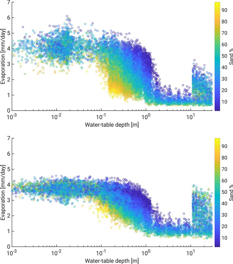
Figure 1. Location of the Neckar catchment within SW Germany.
and time series of state variables or system parameters ex- model saturated and unsaturated flow in the subsurface and
tracted from the simulated catchment and compare them to the fully integrated kinematic wave equation to model two-
observations in the real Neckar catchment to demonstrate dimensional overland flow. Other global and regional hy-
how well the most important requirements are met. These re- drological models also use the latter to route overland flow,
sults as well as possible ways to improve them are discussed e.g., MODCOU (Haefliger et al., 2015) and TRIP (Alkama et
in Sect. 5, together with several issues which came up dur- al., 2012). Advanced Newton–Krylov multigrid solvers are
ing the development phase. We provide conclusions and an used that are especially suitable for massively parallel com-
outlook in Sect. 6. puter environments. Excellent model performance and paral-
lel efficiency have been documented by Jones and Woodward
(2001), Kollet and Maxwell (2006), and Kollet et al. (2010).
2 The Terrestrial Systems Modeling Platform A unique feature of ParFlow is the use of an advanced oc-
tree data structure for rendering overlapping objects in 3-D
We used the Terrestrial Systems Modeling Platform space which facilitates modeling complex geology and het-
(TerrSysMP; see Shrestha et al., 2014; Gasper et al., 2014; erogeneity as well as the representation of topography based
Sulis et al., 2015) developed within the Transregional Col- on digital elevation models and watershed boundaries.
laborative Research Centre TR32 (Simmer et al., 2015) for CLM is a single-column biogeophysical land-surface
the generation of the simulated catchment. TerrSysMP cou- model released by the National Center for Atmospheric Re-
ples (Fig. 1 in Gasper et al., 2014) the hydrologic flow model search (NCAR) which considers coupled snow, soil, and veg-
ParFlow v693 (Ashby and Falgout, 1996; Jones and Wood- etation processes. Land-surface heterogeneity is represented
ward, 2001; Kollet and Maxwell, 2006), the land-surface as a nested subgrid hierarchy in which grid cells are com-
Community Land Model (CLM) v3.5 (Oleson et al., 2008), posed of multiple land units (glacier, lake, wetland, urban,
and the atmospheric Consortium for Small-scale Modeling and vegetation), snow/soil columns (to capture variability in
(COSMO v4.21, Baldauf et al., 2011) model via the Ocean snow and soil states within each land unit), and plant func-
Atmosphere Sea Ice Coupling framework (OASIS3) (e.g., tional types (PFTs) to capture the biogeophysical and bio-
Valcke, 2006) using a dynamical two-way approach includ- geochemical differences between broad categories of plants
ing down- and upscaling algorithms for fluxes and state vari- in terms of their functional characteristics. In TerrSysMP, the
ables between computational grids of different resolutions. 1-D Richards equation model included in CLM is replaced
ParFlow is a variably saturated watershed flow model by ParFlow.
which solves the three-dimensional Richards equation to
https://doi.org/10.5194/essd-13-4437-2021 Earth Syst. Sci. Data, 13, 4437–4464, 2021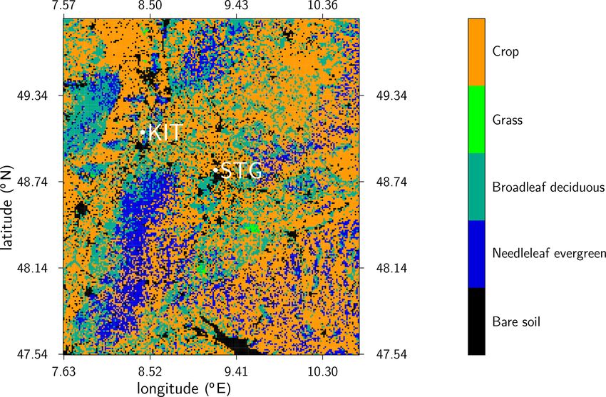
4440                                               B. Schalge et al.: Atmosphere–land-surface–subsurface simulation dataset

   COSMO is a limited-area non-hydrostatic numerical                pled model components. For example, a temporal resolution
weather prediction model, which operationally runs at the           of 15 min is sufficient for the subsurface and land-surface
German weather service (Deutscher Wetterdienst, DWD),               components, whereas time steps as small as 5 s are needed for
among others, for numerical weather prediction (NWP) and            the atmosphere. A higher spatial resolution can be assigned
various scientific applications on the meso-β and meso-             for the surface and subsurface parts to allow for a better rep-
γ scales. COSMO is based on the primitive thermo-                   resentation of soil and land-use heterogeneity.
hydrodynamical equations describing compressible flow in               Since high-resolution and long time series of the fully
a moist atmosphere. As a limited-area model, COSMO                  coupled system are needed to satisfy our need to check the
needs lateral boundary conditions from a driving larger-scale       statistical behavior of the system, the models were run on
model. We impose the lateral conditions by nesting COSMO            the IBM/BlueGeneQ system JUQUEEN at the Jülich Su-
in COSMO-DE, which spans Germany. At the lateral bound-             percomputing Centre (Jülich Supercomputing Centre, 2015).
aries, a relaxation technique is used in which the internal         JUQUEEN has a total of 28 672 nodes with 16 cores each.
model solution is nudged against an externally specified solu-      Our configuration involved using 256 nodes for 12 h, restart-
tion over a narrow transition zone between the two domains.         ing the simulation every 7 simulation days. This is neces-
Version 3.5 of CLM that is used here is already relatively old.     sary as the runtime for ParFlow can vary greatly depend-
Even though version 5 was not yet available when we started         ing on the conditions in the catchment. The total number of
our work, it is now and comparison is warranted. Newer ver-         grid cells for the domain is 323 675 per model layer, with 10
sions of CLM have several major improvements over v3.5.             layers for CLM and 50 layers for ParFlow, and 58 420 grid
The first one is a more sophisticated routing scheme, leading       points for the 50 COSMO layers, resulting in 22.3 million
to much improved soil moisture profiles. In our case, we re-        grid cells. We ran the fully coupled model for a period of nine
place this part with ParFlow anyway, so our older version is        years (2007–2015) as 2007 was the first full year where high-
not a disadvantage in that regard. Other improvements are the       resolution atmospheric forcings were available and 9 years
inclusion of carbon and nitrogen cycles, as well as more op-        was the maximum possible simulation length given con-
tions for crop type vegetation. Here, we purposely simplify         straints on compute resources. On average, the actual runtime
our setup, as we not only have and want static land use but         was approximately 8 h. This means that for 1 year of simu-
also use a blend type of crop with no sharp changes in leaf         lation roughly 1.7 million core hours are needed. For the full
area index (LAI) due to harvests. Instead, we assume harvest        9-year time series, that is about 12 million core hours; an-
to be an ongoing process all throughout autumn. Thus, all           other ∼ 8 million hours were needed for the spin-up. We used
these improvements do not downgrade the simulation results          an output interval of 15 min, which results in a total output
presented and discussed in this study.                              of 38.5 TB of data for the full time series, where about half
   Within OASIS3, the upscaling algorithm uses the mosaic           was produced by COSMO and a quarter each by CLM and
or explicit subgrid approach (Avissar and Pielke, 1989) in          ParFlow.
which high-resolution land-surface fluxes are averaged and
transferred to the coarser resolution of the atmospheric model
component. The implemented Schomburg scheme (Schom-                 3   Description of the virtual Neckar catchment
burg et al., 2010, 2012) downscales atmospheric variables of
the lowest atmospheric model layer to the higher-resolved           Our simulated catchment is based on the Neckar catchment
land-surface model. The scheme involves (i) spline interpo-         in southwestern Germany (see Fig. 1), east of the Black For-
lation while conserving mean and lateral gradients of the           est mountain range and north of the Jurassic ridge of the
coarse field, (ii) deterministic downscaling rules to exploit       Swabian Alps. The catchment has a varying topography in-
empirical relationships between atmospheric variables and           cluding mountains up to 1050 m a.s.l., river valleys, differ-
surface variables, and (iii) the addition of high-resolution        ent land-use types, i.e., grassland, cropland (majority of the
variability (i.e., noise) in order to honor the non-deterministic   area), broadleaf and needle leaf forest (see Fig. 3), and rela-
part and to restore spatial variability.                            tively large soil spatial variability. Annual mean precipitation
   TerrSysMP allows simulating the terrestrial water, en-           over the real catchment ranges between 500 and 2000 mm
ergy, and biogeochemical cycles from the deeper subsurface          (see Sect. 5.1), with the highest values over the Black For-
including groundwater (ParFlow) across the land-surface             est. Interannual variability of precipitation can reach up to
(CLM) into the atmosphere (COSMO). Water and energy                 one-third of the mean value. Monthly precipitation can vary
cycles are coupled via evaporation and plant transpiration;         largely, and its mean annual cycle is weak with slightly lower
these processes are modeled by CLM with a non-linear cou-           values in spring and autumn. While summer precipitation
pling to ParFlow through soil-water availability and root-          is dominated by convection, winter precipitation is predom-
water uptake (Fig. 2). The two-way coupling between CLM             inantly related to fronts of extratropical cyclones with en-
and COSMO encompasses radiation exchange and turbulent              hanced precipitation over the mountains due to orographic
exchanges of moisture, energy, and momentum. OASIS3 al-             lift. Daily average temperatures vary with altitude between
lows for different temporal and spatial resolutions of the cou-     −5 and 0 ◦ C in January and between 13 and 18 ◦ C in July.

Earth Syst. Sci. Data, 13, 4437–4464, 2021                                          https://doi.org/10.5194/essd-13-4437-2021
B. Schalge et al.: Atmosphere–land-surface–subsurface simulation dataset                                                         4441

Figure 2. Land cover in the simulated domain covering the entire Neckar catchment and bounding areas. KIT: Karlsruhe Institute of Tech-
nology (location of meteorological tower observations), STG: Stuttgart (location of radiosonde observations).

                                                                      Land use and cover in the lower elevations are dominated by
                                                                      agriculture, while the Black Forest features mainly needle-
                                                                      leaf trees. Broadleaf trees can be found over smaller areas
                                                                      throughout the catchment. The distance to groundwater is in
                                                                      large parts of the area restricted to a few meters, in particu-
                                                                      lar in lowland areas, which assures strong coupling between
                                                                      the groundwater table and evapotranspiration (Maxwell et
                                                                      al., 2007). These typical central European catchment features
                                                                      in addition to the relatively shallow groundwater tables (im-
                                                                      plying a stronger possible feedback of groundwater on atmo-
                                                                      spheric conditions) were the basis to select the Neckar catch-
                                                                      ment for our simulation.
                                                                         The computational domain is a rectangular area of
                                                                      ∼ 57 850 km2 encompassing the Neckar catchment of ∼
                                                                      14 000 km2 . The domain is larger than the Neckar catchment
                                                                      in order to allow the atmospheric model to develop its own
                                                                      internal dynamics. COSMO is run on a 1.1 km horizonal grid
                                                                      with 230 × 254 grid points, which includes a four-grid-point-
                                                                      wide outer frame zone where only the lateral boundary forc-
                                                                      ing is used without coupling to the CLM, as well as 50 verti-
                                                                      cal layers in hybrid coordinates (terrain following at the sur-
                                                                      face, flat in the stratosphere). COSMO is set up identical to
                                                                      the operational COSMO-DE setup of the German national
                                                                      weather service (DWD); e.g., the deep convection parameter-
Figure 3. Daily average evaporation simulated for 30 April (too)      ization is switched off because at the chosen grid resolution
and 31 July 2007 (bottom) in mm d−1 . The color indicates soil sand   convection is enabled by the dynamical core (see Sect. 2.1).
percentage.
                                                                      In COSMO-DE, the operational resolution is 2.8 km, so that
                                                                      the approximation regarding deep convection is even more

https://doi.org/10.5194/essd-13-4437-2021                                            Earth Syst. Sci. Data, 13, 4437–4464, 2021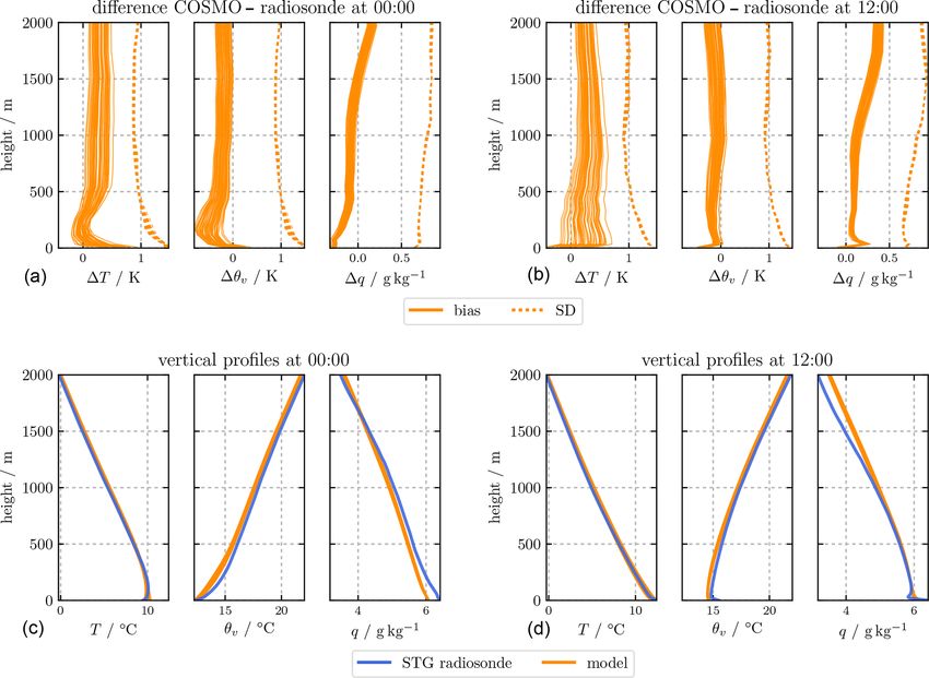
4442                                             B. Schalge et al.: Atmosphere–land-surface–subsurface simulation dataset

appropriate in our simulations. Similar choices were taken        soil. Water surfaces (e.g., larger lakes like Lake Constance in
by Smith et al. (2015), who simulated precipitation events of     the south of the domain) are also treated as bare soil in CLM,
roughly the same domain using nested WRF models, where            while COSMO uses its own land mask and specific calcula-
the cumulus parameterization was switched off at horizon-         tions for water surfaces. Therefore, no values from CLM are
tal resolutions of 900 and 300 m. Lateral boundary forcing        used for water surfaces in COSMO. A few hundred grid cells
and constant fields (topography, land mask, etc.) are pro-        feature shrubs (mostly areas that are re- or deforested or ar-
vided by the COSMO-DE analysis fields, which are down-            eas at higher altitudes) which are treated as forests, and each
scaled to the 1.1 km grid by linear interpolation. The lateral    grid cell features only one – the most dominant – plant func-
relaxation zone, which moderates the jump from the lateral        tional type. The plant LAI is computed from MODIS (My-
driving fields to the inner model area, is set to 12 km.          neni et al., 2002) as monthly averages for the year 2008 for
   A software restriction (unfixable bug specific to the super-   each of the four vegetated land-use classes. As a result, inter-
computing system we were using for our simulation runs as         annual variability is not considered in this simulation, as we
described in the previous section) did not allow for cases with   have the same LAI curve for each PFT each year. This some-
more than 4.2 million CLM columns, as the model did not           what limits the comparability to ET observations especially
initialize properly and crashed, implying that a higher spa-      in spring. This LAI is increased for all plant functional types
tial resolution for CLM and ParFlow than 400 m could not          by 20 % on average (more for forests and less for grassland
be achieved for the Neckar catchment on the used system.          and crops) in the summer months and significantly changed
So, ParFlow and CLM use the same horizontal grid with a           from factors of less than 1 to 3.3 in wintertime (DJF aver-
resolution of 400 m and 535 × 605 grid points. The vertical       age) for needleleaf forests in order to account for known bi-
grid for both component models is partially the same, with        ases in the MODIS data (Tian et al., 2004). This is mostly
CLM limited to 10 vertical layers up to a total depth of 3 m      related to snow cover and fractional land cover due to the
shared with ParFlow, which has in total 50 vertical layers        satellite footprint which often includes other vegetation types
reaching down to 100 m. COSMO runs with a 5 s time step,          or roads and other buildings, leading to an underestimation
while CLM and ParFlow run at 15 min time steps, which is          for a grid cell that is fully covered by just one type as we
also the coupling frequency.                                      have used. The stem area index (SAI) is estimated from the
   For setting up CLM, the European digital elevation             LAI by a slightly modified (no dead leaves for crops, con-
model (DEM) by the European Environment Agency (EEA)              stant base SAI of 10 % of the maximum LAI) formulation of
(http://www.eea.europa.eu/data-and-maps/data/eu-dem, last         Lawrence and Chase (2007) and Zeng et al. (2002) to better
access: 1 October 2017) was projected to the latitude–            represent European tree types. Vegetation height was set to
longitude grid and bi-linearly interpolated to 400 m from         7 m for needleleaf trees and 10 m for broadleaf trees to ac-
the original 30 m spatial resolution. The same DEM is used        count for partial coverage by shrubs, to 20–120 cm for crops,
to create the slope input files for ParFlow. A slight modi-       and to 10–60 cm for grass depending on the time of the year
fication to the original DEM was made in order to ensure          with low values in the winter months and largest values in
that the simulated Neckar River would flow in the correct         July and August. Since we consider only one crop type, we
valley, especially in the upper half of the catchment where       do not specify a harvest date when the plant height drops to
the valley is not always properly resolved by the 400 m           its minimum but assume a smooth decline between August
resolution. In total, the elevation of eight grid points was      and October.
reduced to achieve proper routing for the Neckar River.              For the representation of soils in CLM, we use the
The resulting elevation map is part of the CLM input data         1 : 1 000 000 soil map (BUEK1000, roughly 1 km resolution)
and is available with the dataset as supplementary mate-          provided by the Federal Institute for Geosciences and
rial (https://cera-www.dkrz.de/WDCC/ui/cerasearch/entry?          Natural Resources (BGR) (http://www.bgr.bund.de/DE/
acronym=Neckar_VCS_v1_FORCING, last access: 9 Au-                 Themen/Boden/Informationsgrundlagen/Bodenkundliche_
gust 2021). We have not considered rivers outside the Neckar      Karten_Datenbanken/BUEK1000/buek1000_node.html, last
catchment in these corrections; thus, there are cases where       access: last access: 29 July 2021). This soil map is available
their routing is not identical to the real rivers.                for all of Germany; thus, only small areas in Switzerland and
   Land use is taken from the 2006 CORINE Land                    France are missing outside the Neckar catchment for which
Cover Data Set (https://land.copernicus.eu/pan-european/          we assume a nearby soil class. BUEK1000 offers sand and
corine-land-cover/clc-2006, last access: 29 July 2021) also       clay percentages as well as carbon content for two to seven
provided by EEA. Since the latter dataset features many           soil horizons down to a maximum depth of 3 m for each soil
more land-use types (at a resolution of 100 m) than required      type. The carbon content is used to infer soil color. For urban
by CLM, they were grouped according to the CLM (In-               areas (modeled as bare soil, as mentioned above) a fixed soil
ternational Geosphere-Biosphere Programme, IGBP) plant            color (class 8 in CLM) was used.
functional type classes (1) broadleaf forests, (2) needleleaf        Since soil properties may vary substantially at scales
forests, (3) grassland, (4) cropland, and (5) bare soil. Urban    smaller than the 1 km for which BUEK1000 is appropriate,
areas are not considered in this setup and replaced by bare       which might impact system dynamics (Binley et al., 1989;

Earth Syst. Sci. Data, 13, 4437–4464, 2021                                        https://doi.org/10.5194/essd-13-4437-2021
B. Schalge et al.: Atmosphere–land-surface–subsurface simulation dataset 4443
Herbst et al., 2006; Rawls, 1983), the soil map is downscaled In order to keep soil porosity identical between CLM and
by artificially adding variability using the conditional points ParFlow, we replaced the porosity calculation within CLM
method recently presented in Baroni et al. (2017) as follows: (which uses a different pedotransfer function). The Man-
ning’s surface roughness was set to a constant value of
1. The BUEK1000 soil map is randomly sampled at 1995 5.52×10⁻⁴ h m−1/3 and the specific storage to 1×10⁻³ . The
point locations with one sample every 5 km2 on average, chosen surface roughness value results in a realistic base flow
a minimum sample distance of 250 m, and at least one for the local rivers without calibration. Repercussions of this
sample for each soil type of the original soil map, which choice are discussed in Sect. 6. Slopes of the main rivers are
is realistic in the context of how soil maps are usually additionally smoothed to avoid artificial ponded areas.
created. This strategy resulted from extensive testing by All these changes are part of the forcing files that are
minimizing the tradeoffs between reproducing the main provided with the full dataset, making it easy to repro-
features of the original soil map and creating variability duce our simulations (https://cera-www.dkrz.de/WDCC/ui/
at finer resolution. cerasearch/entry?acronym=Neckar_VCS_v1_FORCING,
last access: 29 July 2021).
2. The sample locations are used as conditional points for
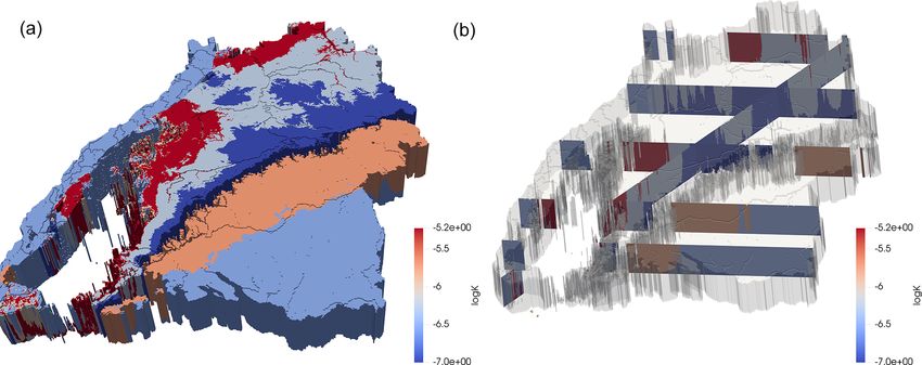
In order to allow for realistic flow in the saturated zone,
further interpolation. Here, texture, carbon content, and
the 3-D geologic model of the geological survey of the state
depth of the first three soil horizons are extracted from
of Baden-Württemberg was used from which 11 rock types
the BUEK1000, resulting in variable soil depth rather
were defined for Baden-Württemberg (see Fig. A1). Some
than the assumed unrealistic uniform soil depth. In addi-
characteristic features of the domain, such as middle Tri-
tion, the sand content of the original map was increased
assic and Jurassic karst aquifers, are not included to avoid
by 20 % (except for areas with very high sand content
the manifold hydrological challenges related to its model-
to avoid grid cells with > 90 % sand), resulting in a
ing. While this can have a significant impact on ground-
slightly higher hydraulic conductivity because previous
water representation in the karst areas, for the rather short
simulations yielded too-shallow unsaturated zones re-
time period considered here, we expect a limited impact
lated to the spatial resolution of the simulation. Chang-
on near-surface soil moisture content as the affected areas
ing sand content increased the thickness of unsaturated
have in general deeper groundwater levels. For areas outside
zones and lowered groundwater tables, fixing most of
of Baden-Württemberg, we extended the rock types at the
the emerging biases.
boundary outwards to cover the full computational domain.
3. Experimental variograms and cross-variograms are cal- Table 1 summarizes porosity and hydraulic conductivity used
culated for all variables, and exponential models were in the domain for the different stratigraphic units. Since karst
fitted to all spatial structures. features of limestones are not considered, porosities in strati-
graphic units containing limestones and crystalline rocks are
4. A texture map (sand and clay percentage) is gener- set considerably higher than in nature to somewhat counter
ated using a single realization based on conditional co- this.
simulation (Gomez-Hernandez et al., 1993) to provide Not covered by the discussed datasets (not part of the soil
the subscale variability (< 1 km2 ). Soil horizon depths and not large enough to be resolved in the geological map)
and carbon content are, however, assumed to have a are the large alluvial bodies filling large part of the Neckar
smoothed spatial variability; therefore, they are interpo- valley throughout the domain (Riva et al., 2006). Up to 30 %
lated based on ordinary kriging as the removal of small- of the runoff takes place in the subsurface, especially dur-
scale variability is not important for the depth and car- ing periods of base flow, according to a subcatchment sim-
bon content. ulation performed for the year 2007. In that simulation, we
used measured precipitation and river discharge data together
5. Since ParFlow describes retention and hydraulic con- with the simulated evapotranspiration to calculate the water
ductivity curves based on Mualem–van Genuchten pa- balance over a whole year. While our simulated evapotran-
rameters, pedotransfer functions are applied to estimate spiration rates may be inaccurate, it is implausible that this
these parameters. The pedotransfer function of Cosby et can account for 30 % of the precipitation, as in this climate
al. (1984) is used to estimate saturated hydraulic con- we are almost always energy limited, and therefore ET errors
ductivity based on soil texture, the one from Rawls will be smaller and mostly related to errors in atmospheric
(1983) is used to estimate soil bulk density based on forcings and LAI. This implies that the water could only
soil texture and organic matter, and the one from Tóth have left the domain through the subsurface. Thus, gravel
et al. (2015) is used to estimate van Genuchten param- channels are needed to account for this lateral flow. Since
eters based on soil texture and bulk density. These have the valleys in the catchment are often small compared to the
been selected based on data availability, applicability of limited horizontal resolution of the model, we conceptualize
the particular approaches, and previous evaluations con- the alluvial bodies as gravel layers underneath all river cells
ducted in the area (Tietje and Hennings, 1996). (cells with a mean pressure head > 0.1 m) and directly next
https://doi.org/10.5194/essd-13-4437-2021 Earth Syst. Sci. Data, 13, 4437–4464, 2021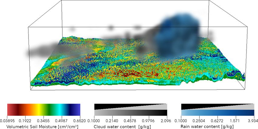
4444                                               B. Schalge et al.: Atmosphere–land-surface–subsurface simulation dataset

to rivers (riverbanks, i.e., one grid point besides each river      metric soil moisture. The soil exhibits different soil moisture
cell). The assumed gravel layers reach from beneath the soil        layers, the variability of which is mainly connected to dif-
down to a depth of 8 m. The gravel cells are parameterized          ferent soil hydraulic properties. Only clouds reaching high
with a high hydraulic conductivity of 1 m h−1 , a porosity of       enough to have sufficient cloud ice produce precipitation, and
0.6 and van Genuchten parameters of 2 for n and 4 m−1 for α         some precipitation evaporates before it reaches the ground.
(residual saturation is 0.06 cm3 cm−3 ). Our setup results in a     Extended weather fronts moving through the domain (not
reasonable distribution of surface and subsurface discharge at      shown), which are imposed by the boundary conditions, are
the outlet of the catchment and reasonable river–aquifer ex-        also simulated realistically (timing, strength of wind gusts,
change fluxes. In addition to the gravel channels, we included      change of wind direction, change in temperature and pres-
a layer of weathered bedrock, which starts below the soil and       sure) given the resolution of the atmospheric model.
extends down to a depth of 6 m. This layer is characterized
by substantially larger porosity (0.4) and hydraulic conduc-        4.1   Relation between water table depth and
tivity (0.1 m h−1 ) than the rock below. This layer was added             evapotranspiration
to enhance subsurface flow and counter the common occur-
rence of too-shallow water levels if these features are not in-     An important measure for hydrometeorological interactions
cluded. Both these changes are realistic when compared to           within a catchment is the relation between water availabil-
the actual morphology of the Neckar river valley. While it is       ity and surface energy flux partitioning. Thus, the simulated
quite narrow in many places, there are still significant allu-      catchment should capture the expected reduced evapotran-
vial deposits everywhere except the furthest upstream region        spiration (ET) with increasing distance to groundwater (e.g.,
(which are not considered for this anyway due to the pres-          Maxwell et al., 2007; Shrestha et al., 2014). In Fig. 3, we
sure cutoff). The choice for the weathered bedrock layer is         show daily averaged evaporation (which here is equal to
also reasonable given the temperature and moisture ranges           ET as all other contributors are zero) values over bare soil
leading to imperfections in the rock layers near the surface.       against distance to groundwater for 30 April and 31 July
   Since we enforce no-flow boundary conditions at the sub-         for the year 2007. These days were chosen as they were
surface domain boundaries, all water has to eventually reach        preceded with several dry days in almost the whole catch-
the surface in order to leave the domain. This happens pre-         ment, leading to comparable states for the upper soil lay-
dominantly in areas outside of the Neckar catchment, e.g., in       ers. April was almost completely dry (on average less than
the upper Rhine Valley; thus, soil moisture values in this re-      3 mm precipitation over the domain), while July was much
gion may be too high.                                               wetter, but the increased solar radiation and thus tempera-
                                                                    tures compared to April result in higher evaporation rates
                                                                    and thus a quicker drying of the top layer of the soil. Fig-
4   Results                                                         ure 3 indicates a reduction in evaporation when the distance
                                                                    to groundwater falls below 15–100 cm, depending on soil
In the following, we present example results of the                 properties with faster evaporation reduction for increasing
simulated-reality simulations in order to demonstrate its po-       soil sand content. Such relations are less obvious for cells
tential for a better understanding of the dynamics in coupled       with significant plant cover: while trees show overall higher
terrestrial systems. We will also show that the simulations         evaporation and almost no change with distance to ground-
quite well resemble observations in the real Neckar catch-          water due to their deep root zones, variability increases with
ment, and thus can be used to develop and evaluate modeling         larger distances to groundwater (not shown). Also crops and
and prediction strategies. Precipitation is the strongest hy-       grassland show limited evaporation changes as a function of
drological driver in this region; thus, its realistic spatial and   distance to groundwater, which can, however, be explained
temporal variability in the domain including its statistical re-    by the high water availability (no water stress) in the time
lations with topography is important. Also, the state of the        period considered. Figure 3 also contains a small number
atmospheric boundary layer, which reflects the interaction of       of grid points at a water table depth of 7 m or deeper, with
the land surface with the atmosphere, is a critical component       evaporation rates only slightly lower than in the shallow wa-
of the terrestrial system, which should be represented by the       ter table regions. These relate most likely to cells that retain
simulation with some confidence. Along with the compar-             high levels of upper-level soil moisture even during dry pe-
isons, we will also discuss the challenges experienced with         riods to support higher evaporation. This could be due to the
such a modeling setup.                                              way the water table is calculated. We define the water table as
   Even though we do not aim to be as close to reality as           the deepest threshold between positive and negative pressure.
possible, we feel it is important to show that the model sys-       Since there are some places where there is another saturated
tem is behaving as expected and is thus suitable for the var-       region closer to the surface, leading to higher water availabil-
ious use cases we discussed. Figure A2 shows as an exam-            ity near the surface, the high value for the water table can be
ple result a snapshot of the simulated three-dimensional dis-       misleading with respect to near-surface soil moisture. Such
tribution of cloud water/ice, precipitation density, and volu-      a feature will only occur if the water table is deep enough

Earth Syst. Sci. Data, 13, 4437–4464, 2021                                          https://doi.org/10.5194/essd-13-4437-2021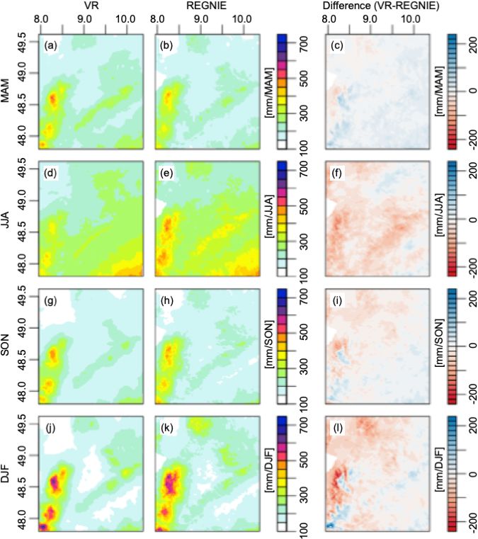
B. Schalge et al.: Atmosphere–land-surface–subsurface simulation dataset                                                   4445

to begin with, which is why we do not see this for water ta-     simulated winter precipitation (Fig. 5b) do not show a diurnal
bles of less than 10 m. As a result, volumetric soil moisture    cycle, summer precipitation (Fig. 5a) increases over the after-
for these cells with deep water table but high evaporation is    noon reaching a maximum at about 19:00 LT in accordance
much more similar to cells with a shallow water table than to    with the maximum of convective precipitation. The simula-
cells with a deep water table but low evaporation.               tions reproduce this pattern but exhibit a weak second peak
   We want to point out that in this region ET is almost al-     between 06:00 and 12:00 LT while the afternoon–evening in-
ways limited by atmospheric demand, which is why we limit        crease is delayed by about 2 h. The simulated daily precipi-
the analysis to bare-soil evaporation only. Since the upper-     tation distribution fits the observations especially in late af-
most layers can dry quickly, the resulting drop in evaporation   ternoon and night, while it overestimates precipitation during
can be seen, which is not the case for ET if there is an ex-     the late morning and underestimates it in early afternoon in
tended root zone as we have for crops, grassland and forests.    summer. In winter, this effect is much less pronounced. This
These bare-soil areas are not a feature of the real catchment    behavior is related to the representation of convective show-
and as such cannot be compared to real measurements.             ers in the atmospheric model. The responsible parametriza-
                                                                 tion was not designed for the kilometer scale and application
4.2   Precipitation
                                                                 at this resolution results in a too-early onset of convective
                                                                 precipitation. While the simulated catchment has somewhat
We compare the simulated precipitation with the 1 ×              fewer dry and low precipitation days than REGNIE, the num-
1 km gridded REGNIE (Regionalisierung der Nieder-                ber of days between 4 and 10 mm are higher than in REGNIE
schlagshöhen) product of DWD, derived from in situ precip-       (not shown). The simulated and observed seasonal precipita-
itation observations (Rauthe et al., 2013). For the evaluation   tion cycles (Fig. 6) compare very well, and mean precipi-
of seasonal daily precipitation cycles, hourly observations of   tation is nearly identical between simulations and observa-
71 DWD observational stations are used. The simulated sea-       tions. The model reproduces the seasonal cycle of maximum
sonal mean precipitation (Fig. 5) and the annual mean pre-       daily precipitation well, however with larger differences in
cipitation (not shown) are governed by the orographic struc-     the summer (see also Dierer et al., 2009).
tures of the Black Forest and Swabian Alps. Values range
between approximately 520 mm yr−1 around Mannheim and            4.3   Atmospheric state variables and surface radiation
2105 mm yr−1 over the Black Forest in good accordance with
REGNIE concerning the overall pattern and range (510–            We compare the atmospheric boundary layer (ABL) of the
2130 mm yr−1 ). Overall, the simulation shows about 10 %         simulated catchment to observations from the meteorologi-
higher annual precipitation in the east and south and about      cal tower at Karlsruhe Institute of Technology (KIT; Kalthoff
25 % lower in the north and west compared to REGNIE.             and Vogel, 1992) and with DWD radiosonde observations in
During winter (December to February), precipitation is dom-      Stuttgart (STG) (see Fig. 1 for locations and Table A1 for
inated by advection from the west, which results in max-         details of observed quantities). To avoid a biased compari-
ima over the upwind and peak zones of the mountains and          son related to land-cover mismatches between the simulation
leeward minima. The simulated winter pattern (j ) compares       and the actual land use at the observation sites, the simula-
well with REGNIE (k), but the model underestimates pre-          tion results are averaged over five-by-five atmospheric grid
cipitation in the northwestern part of the catchment (l). Over   boxes centered around the observation sites, thus giving ap-
the mountains, a slight lateral shift of this kind of precipi-   proximately the same fractional land cover as is present at
tation pattern results in neighboring areas with under- and      the observation location.
overestimation also found for COSMO simulations coupled             The 10 m mean diurnal minimum temperatures in the
to its own TERRA land-surface model (e.g., Dierer et al.,        catchment are between 0.5 K (January) and 2.5 K (August)
2009; Lindau and Simmer, 2013). In fall, the difference pat-     higher than observed (Fig. 7, top) and are reached approxi-
tern between simulations and REGNIE (i) is similar to the        mately 1 h later than observed with the subsequent morning
winter pattern but has smaller contrasts. In spring, the sim-    temperature rise shifted accordingly. The simulated diurnal
ulated precipitation is higher compared to REGNIE. In the        temperature maxima are on average 0.7 K lower than in the
summer (June to August), cloud bases are usually higher and      observations and are reached 30 min later than measured. The
reduce the patterns caused by the luff–lee effects. Moist air    morning temperature gradient in the simulation ranges from
extends further to the east and south and gets staunched by      0.10 K h−1 in December to 0.31 K h−1 in April, which com-
the alpine upland, leading to enhanced precipitation there.      pares reasonably well with the observations (0.13/0.52 K h−1
The simulated summer precipitation pattern, which is dom-        in January/April). The evening cooling, however, progresses
inated by convective precipitation, resembles the REGNIE         too slowly and results in too-high minimum temperatures.
pattern but exceeds the latter by being 20 % lower over large    At 100 m above the ground, diurnal maximum temperatures
parts of the catchment (Fig. 4).                                 agree within 0.7 K, while the warm bias of diurnal mini-
   The mean seasonal diurnal precipitation cycles (Fig. 5) re-   mum temperatures (0.9 K) is smaller than at 10 m height
flect the dominating precipitation types. While observed and     (Fig. 7, bottom). Also at 100 m, a 1 h shift between the diur-

https://doi.org/10.5194/essd-13-4437-2021                                       Earth Syst. Sci. Data, 13, 4437–4464, 2021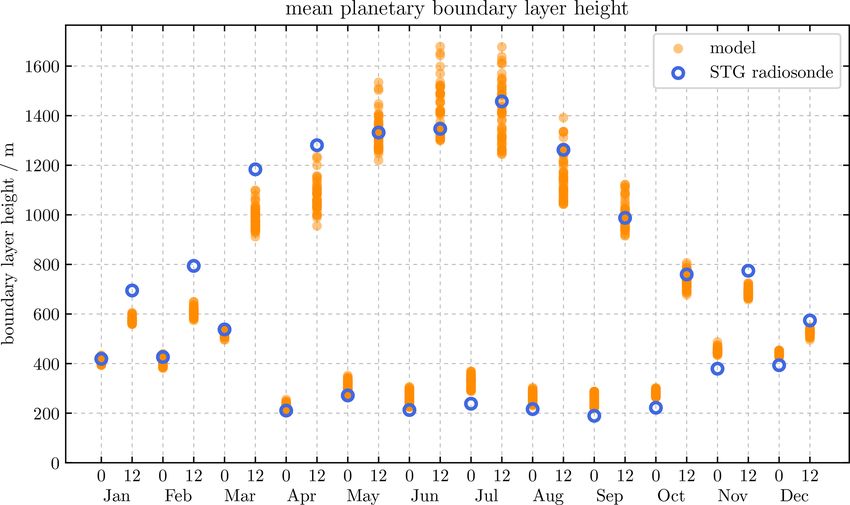
4446                                              B. Schalge et al.: Atmosphere–land-surface–subsurface simulation dataset

Figure 4. Mean seasonal precipitation over the Neckar catchment between 2007–2013 in the simulated reality (VR, left column) compared
to the REGNIE dataset (middle column). The difference between VR and REGNIE is shown in the right column. Panels (a)–(c) show
the comparison for spring (March–May); (d)–(f) for summer (June–August); (g)–(i) for fall (September–November); and (j)–(l) for winter
(December–February).

nal minimum temperatures and the morning temperature rise               COSMO in TerrSysMP estimates ABL heights via the
is found. At a height of 200 m, the simulated monthly mean           bulk Richardson number criterion with a threshold of 0.22
diurnal cycles are practically identical to the KIT observa-         for unstable and 0.33 for stable conditions (Szintai and Kauf-
tions (not shown). The simulated temperature standard devia-         mann, 2008). Both seasonal and diurnal variations of the
tions (mean absolute difference for each time of day between         mean ABL height at 00:00 and 12:00 LT agree well with the
the specific daily value and the corresponding monthly mean;         observations using the same criterion (Fig. 8), but the sim-
see Appendix Eq. (A1) for details) are somewhat smaller              ulation tends to overestimate ABL heights during nighttime
than observed, especially in afternoons in the summer half           by up to 150 m and underestimate it during daytime by up
year with underestimations of the temperature standard devi-         to 200 m in March. Figure 9 compares simulated mean verti-
ation larger than 20 %.                                              cal profiles of temperature, virtual potential temperature, and
                                                                     specific humidity with radiosonde observations at 00:00 and

Earth Syst. Sci. Data, 13, 4437–4464, 2021                                            https://doi.org/10.5194/essd-13-4437-2021
B. Schalge et al.: Atmosphere–land-surface–subsurface simulation dataset 4447
Figure 5. Mean diurnal precipitation cycle for the 71 DWD sta- Figure 6. (a) Daily precipitation distribution on a monthly basis
tions and the corresponding simulations for wet days (more than as observed (black) and simulated (red). The gray and red lines
1 mm d−1 ) for June–August (a) and December–February (b) sea- indicate the monthly mean precipitation. (b) Maximum daily pre-
sons. The upper and lower hinges correspond to the first and third cipitation for the given months for the 71 DWD stations and the
quartiles, the center black line indicates the median, the upper corresponding simulation. Box sizes as explained in the caption of
whisker (analog for lower whisker) extends from the hinge to the Fig. 10.
highest value within 1.5 · (interquartile range), and the black dots
mark the outliers.
Overall, the atmospheric profiles, including the ABL
heights, are very close to observations during the day and
12:00 LT in STG including the mean differences (bias) and at heights above 10 m. Noteworthy differences only occur
the standard deviation of the differences. Simulations are up close to the surface with too-high nighttime temperatures
to 0.9 K warmer close to the surface at 00:00 LT and up to (up to 2.5 K in summer) and subsequently too-small morn-
0.5 K colder at 12:00 LT. At larger heights, the simulations ing temperature gradients. Somewhat higher incoming short-
are up to 0.5 K warmer depending on land cover. Specific hu- wave and lower incoming longwave radiation at the surface
midity profiles at 00:00 LT are approximately 0.2 g kg−1 too indicate less cloud cover (or lower cloud optical depths) com-
dry close to the surface and 0.2 g kg−1 too wet above 1500 m. pared to the observations. These results are in line with a
At 12:00 LT, profiles are up to 0.3 g kg−1 too wet through- previous evaluation of a 2.2 km COSMO simulation (Ban et
out. The simulations have smaller virtual potential tempera- al., 2014). In addition, we note somewhat reduced unstable
ture gradients and are thus less stable close to the surface at conditions at daytime close to the surface in the simulations.
00:00 LT. At 12:00 LT, the decreasing virtual potential tem-
perature close to the surface is not captured and tends towards
4.4 Passive microwave observations
a more neutral instead of unstable profile at low heights.
At KIT (STG), the land surface receives on average The most direct area-covering observations of soil mois-
20 W m−2 (5.3 W m−2 ) more incoming shortwave radiation ture are currently provided by L-band (1.4 GHz) passive mi-
and 18 W m−2 (8 W m−2 ) less incoming longwave radiation crowave observations from satellites. The Community Mi-
indicating a somewhat lower cloud cover (or lower cloud op- crowave Emission Model (CMEM) is used as a forward op-
tical depth) as observed. During daytime (06:00–22:00 LT), erator to simulate the brightness temperatures (TB) at this
the mean outgoing longwave radiation matches the KIT ob- frequency in vertical and horizontal polarization (de Rosnay
servations, while at nighttime (22:00–06:00 LT) values are et al., 2009). CMEM simulates brightness temperatures at the
7.2 W m−2 larger than observed, which corresponds to a top of the atmosphere resulting from microwave emission
higher surface temperature of approximately 1.4 K. and interaction by soil, vegetation, and atmosphere based
on the state variables of the simulated catchment. Input to
https://doi.org/10.5194/essd-13-4437-2021 Earth Syst. Sci. Data, 13, 4437–4464, 20214448 B. Schalge et al.: Atmosphere–land-surface–subsurface simulation dataset Figure 7. Monthly mean diurnal cycles (local time) and respective standard deviation (see text) for air temperature (◦ C) in 10 m (a) and 100 m (b) height at the KIT tower and for the COSMO grid boxes around the KIT location. Figure 8. Monthly mean boundary-layer height at 00:00 and 12:00 LT for different land covers diagnosed from radiosonde observations at STG and from atmospheric profiles above grid boxes of CLM. Earth Syst. Sci. Data, 13, 4437–4464, 2021 https://doi.org/10.5194/essd-13-4437-2021
B. Schalge et al.: Atmosphere–land-surface–subsurface simulation dataset                                                             4449

Figure 9. Mean vertical profiles of temperature, virtual potential temperature, and specific humidity (a, b), and mean differences between
modeled and observed data including the standard deviation of the differences (c, d). The experimental data are from the radiosonde data at
STG and the simulated data from the grid boxes of the simulated catchment with different land cover (a, c: 00:00 LT, b, d: 12:00 LT).

CMEM are the percentages of clay and sand in the soil, the              ator in TerrSysMP is able to also replicate the NASA SMAP
coverage with open water surfaces, the profiles of soil mois-           (Soil Moisture Active Passive) radiometer (Saavedra et al.,
ture and soil temperature, vegetation types, and LAI. Satellite         2016) for years beyond 2015 (since the time SMAP data have
orbit geometry, antenna pattern, footprint, and incidence an-           been available).
gle are taken into account following the ESA Soil Moisture                 We evaluate the simulated brightness temperature distribu-
and Ocean Salinity (SMOS) instrument specifications; i.e., a            tion over the domain with real SMOS observations between
full-width-half-maximum field of view leading to a footprint            April 2011 and September 2011. The SMOS observations
of 40 km across orbit and 47 km along orbit at multiple in-             are corrected from radio-frequency interference (RFI) ef-
cidence angles (Kerr et al., 2001) is applied. This antenna             fects over the region following Saavedra et al. (2016). Initial
pattern weighs the grid-cell-simulated brightness tempera-              results with CMEM-adapted parameters for surface rough-
tures (Fig. 11, left) in order to obtain simulated SMOS ob-             ness and vegetation optical thickness (which needed to be in-
servations. Finally, these synthetic observations are rendered          creased from its standard values found in the literature) lead
according to pixels based on the icosahedral Snyder equal               to a systematic underestimation of the brightness tempera-
area (ISEA) projection at a spatial separation of about 15 km           ture of about −20 K on average (see orange line in Fig. A3,
similar to the SMOS L1C TB data product (Fig. A4, right),               which compares real SMOS observations with the simulated
which can then be compared with observations for an indi-               brightness temperatures) and maximum and minimum differ-
rect evaluation of the simulation. Every pixel corresponds to           ences of −33 and −6 K, respectively, for an incidence angle
a fixed geolocation of the real SMOS L1C data product over              of 30◦ . A similar underestimation of −14 K resulted for the
the modeled area. Optionally, the satellite observation oper-           40◦ incidence angle with maximum and minimum values of

https://doi.org/10.5194/essd-13-4437-2021                                               Earth Syst. Sci. Data, 13, 4437–4464, 2021
4450                                               B. Schalge et al.: Atmosphere–land-surface–subsurface simulation dataset

Figure 10. Area-averaged L-band brightness temperature the period from April to September 2011 for an incidence angle of 30◦ (a) and
40◦ (b). The boxplots indicate the real SMOS observations averaged over the same domain. The black line is the median of the observations
simulated with CMEM. The dark gray area corresponds to the interquartile range (IQR), while the light gray area encompasses the 3 % to
97 % range. The continuous orange line indicates the brightness temperature without taking into account an assumed bias in surface soil
moisture content (see text).

−34 and +15 K (lower plot in Fig. 10). Those differences               stream approximation to better simulate cases with dense
are mainly caused by the too-large near-surface soil mois-             vegetation in the future.
ture values in the simulated catchment. The cumulative dis-               The microwave observations retrieved from the simulated
tribution functions of the satellite-derived soil moisture prod-       catchment show a typical situation encountered in data as-
ucts and the simulated soil moisture suggests an about 63 %            similation; more often than not, there are biases between sim-
higher near-surface soil moisture compared to the satellite es-        ulated and remote-sensing observations. This discrepancy
timates (Saavedra et al., 2016, Fig. 6) with extremes of 44 %          usually has multiple causes, which can relate to the obser-
and 95 %. With that, a daily matching of the cumulative dis-           vations themselves, assumptions in the observation operator
tribution functions of the simulated catchment and satellite           used to simulate the observations, and in the model used to
retrieved soil moisture is performed to find a factor which            generate the system’s state variables entering the observa-
then is assumed to be the soil moisture bias of the simulation         tion operator. Even if these differences cannot be removed,
and is applied as a correction factor. Figure 10 compares true         such observations can be highly valuable for data assimila-
SMOS observations with simulated brightness temperatures               tion as long as temporal tendencies are meaningful informa-
obtained without and with day-to-day correction for the as-            tion. Usually, the bias is statistically corrected, and thus only
sumed soil moisture bias of the simulation. The correction             the information in the temporal and (if meaningful) spatial
decreases the average bias in brightness temperature from              variability of the observations is exploited for moving the
−20 K (−14 K) to about −3 K (−2 K) for the incidence an-               model states towards the true states.
gle of 30◦ (40◦ ) at horizontal polarization. Similar results are
found when the simulations were statistically compared with
observations of later years from the NASA SMAP (Fig. 3 in              4.5   Evaluation of river discharge
Saavedra et al., 2016). The remaining bias can probably be             We compare river discharge in the simulated catchment with
further reduced by fine tuning radiation interaction param-            observations made in the Neckar catchment at the gaging sta-
eters in CMEM and by including orographic effects on the               tions Rockenau, Lauffen, and Plochingen for a 3-year period
effective incidence angle. These biases will be addressed by           from 2007 to 2009 (Fig. 11). The range of the hydrological
an improved exploitation of the uncertainty of the radiation           responses to precipitation in the simulated catchment is sim-
interaction parameters and by including in CMEM a two-                 ilar to the observations, and also during dry periods the be-
                                                                       havior is similar, which is noteworthy since no calibration to

Earth Syst. Sci. Data, 13, 4437–4464, 2021                                              https://doi.org/10.5194/essd-13-4437-2021
You can also read