Evaluation of global terrestrial evapotranspiration using state-of-the-art approaches in remote sensing, machine learning and land surface ...
←
→
Page content transcription
If your browser does not render page correctly, please read the page content below
Hydrol. Earth Syst. Sci., 24, 1485–1509, 2020
https://doi.org/10.5194/hess-24-1485-2020
© Author(s) 2020. This work is distributed under
the Creative Commons Attribution 4.0 License.

Evaluation of global terrestrial evapotranspiration using
state-of-the-art approaches in remote sensing, machine
learning and land surface modeling
Shufen Pan1 , Naiqing Pan1,2 , Hanqin Tian1 , Pierre Friedlingstein3 , Stephen Sitch4 , Hao Shi1 , Vivek K. Arora5 ,
Vanessa Haverd6 , Atul K. Jain7 , Etsushi Kato8 , Sebastian Lienert9 , Danica Lombardozzi10 , Julia E. M. S. Nabel11 ,
Catherine Ottlé12 , Benjamin Poulter13 , Sönke Zaehle14 , and Steven W. Running15
1 International Center for Climate and Global Change Research, School of Forestry and Wildlife Sciences,
Auburn University, Auburn, AL 36832, USA
2 State Key Laboratory of Urban and Regional Ecology, Research Center for Eco-Environmental Sciences,

Chinese Academy of Sciences, Beijing 100085, China
3 College of Engineering, Mathematics and Physical Sciences, University of Exeter, Exeter EX4 4QF, UK
4 College of Life and Environmental Sciences, University of Exeter, Exeter EX4 4RJ, UK
5 Canadian Centre for Climate Modelling and Analysis, Environment Canada, University of Victoria,

Victoria, BC V8W 2Y2, Canada
6 CSIRO Oceans and Atmosphere, GPO Box 1700, Canberra, ACT 2601, Australia
7 Department of Atmospheric Sciences, University of Illinois, Urbana, IL 61801, USA
8 Institute of Applied Energy (IAE), Minato-ku, Tokyo 105-0003, Japan
9 Climate and Environmental Physics, Physics Institute, University of Bern, Bern, Switzerland
10 Climate and Global Dynamics Laboratory, National Center for Atmospheric Research, Boulder, CO 80305, USA
11 Max Planck Institute for Meteorology, Bundesstr. 53, 20146 Hamburg, Germany
12 LSCE-IPSL-CNRS, Orme des Merisiers, 91191, Gif-sur-Yvette, France
13 NASA Goddard Space Flight Center, Biospheric Sciences Laboratory, Greenbelt, MD 20771, USA
14 Max Planck Institute for Biogeochemistry, P.O. Box 600164, Hans-Knöll-Str. 10, 07745 Jena, Germany
15 Numerical Terradynamic Simulation Group, College of Forestry and Conservation,

University of Montana, Missoula, MT 59812, USA

Correspondence: Shufen Pan (panshuf@auburn.edu)

Received: 3 August 2019 – Discussion started: 21 August 2019
Revised: 22 January 2020 – Accepted: 27 January 2020 – Published: 31 March 2020

Abstract. Evapotranspiration (ET) is critical in linking            these three categories of approaches agreed well, with val-
global water, carbon and energy cycles. However, direct mea-        ues ranging from 589.6 mm yr−1 (6.56 × 10⁴ km3 yr−1 ) to
surement of global terrestrial ET is not feasible. Here, we first   617.1 mm yr−1 (6.87 × 10⁴ km3 yr−1 ). For the period from
reviewed the basic theory and state-of-the-art approaches for       1982 to 2011, both the ensembles of remote-sensing-based
estimating global terrestrial ET, including remote-sensing-         physical models and machine-learning algorithms suggested
based physical models, machine-learning algorithms and              increasing trends in global terrestrial ET (0.62 mm yr−2 with
land surface models (LSMs). We then utilized 4 remote-              a significance level of p < 0.05 and 0.38 mm yr−2 with a sig-
sensing-based physical models, 2 machine-learning algo-             nificance level of p < 0.05, respectively). In contrast, the en-
rithms and 14 LSMs to analyze the spatial and temporal vari-        semble mean of the LSMs showed no statistically significant
ations in global terrestrial ET. The results showed that the        change (0.23 mm yr−2 , p > 0.05), although many of the in-
ensemble means of annual global terrestrial ET estimated by         dividual LSMs reproduced an increasing trend. Nevertheless,

Published by Copernicus Publications on behalf of the European Geosciences Union.
1486                                                                        S. Pan et al.: Evaluation of global terrestrial ET

all 20 models used in this study showed that anthropogenic         this is due to the fact that it is modulated not only by sur-
Earth greening had a positive role in increasing terrestrial       face meteorological conditions and soil moisture but also
ET. The concurrent small interannual variability, i.e., rela-      by the physiology and structures of plants. Changes in non-
tive stability, found in all estimates of global terrestrial ET,   climatic factors such as elevated atmospheric CO2 , nitrogen
suggests that a potential planetary boundary exists in regu-       deposition and land covers also serve as influential drivers
lating global terrestrial ET, with the value of this boundary      of Tv (Gedney et al., 2006; Mao et al., 2015; S. Pan et al.,
being around 600 mm yr−1 . Uncertainties among approaches          2018; Piao et al., 2010). As such, the global ratio of transpi-
were identified in specific regions, particularly in the Ama-      ration to ET (Tv /ET) has long been a matter of debate, with
zon Basin and arid/semiarid regions. Improvements in pa-           the most recent observation-based estimate being 0.64±0.13
rameterizing water stress and canopy dynamics, the utiliza-        constrained by the global water-isotope budget (Good et al.,
tion of new available satellite retrievals and deep-learning       2015). Most Earth system models are thought to largely un-
methods, and model–data fusion will advance our predictive         derestimate Tv /ET (Lian et al., 2018).
understanding of global terrestrial ET.                               Global warming is expected to accelerate the hydrolog-
                                                                   ical cycle (Pan et al., 2015). For the period from 1982 to
                                                                   the late 1990s, ET was reported to have increased by about
                                                                   7 mm (∼ 1.2 %) per decade driven by an increase in radia-
1   Introduction                                                   tive forcing and, consequently, global and regional temper-
                                                                   atures (Douville et al., 2013; Jung et al., 2010; Wang et al.,
Terrestrial evapotranspiration (ET) is the sum of the wa-          2010). The contemporary near-surface specific humidity also
ter lost to the atmosphere from plant tissues via transpira-       increased over both land and ocean (Dai, 2006; Simmons et
tion and that lost from the land surface elements, including       al., 2010; Willett et al., 2007). More recent studies confirmed
soil, plants and open water bodies, through evaporation. Pro-      that global ET has showed an overall increase since the 1980s
cesses controlling ET play a central role in linking the en-       (Mao et al., 2015; Yao et al., 2016; Zeng et al., 2018a, 2012,
ergy (latent heat), water (moisture flux) and carbon cycles        2016; Zhang et al., 2015; Y. Zhang et al., 2016). However,
(photosynthesis–transpiration trade-off) in the Earth system.      the magnitude and spatial distribution of such a trend are far
Over 60 % of precipitation on the land surface is returned         from determined. Over the past 50 years, pan evaporation has
to the atmosphere through ET (Oki and Kanae, 2006), and            decreased worldwide (Fu et al., 2009; Peterson et al., 1995;
the accompanying latent heat (λET, λ is the latent heat of         Roderick and Farquhar, 2002), implying an increase in ac-
vaporization) accounts for more than half of the solar en-         tual ET given the pan evaporation paradox. Moreover, the in-
ergy received by the land surface (Trenberth et al., 2009).        crease in global terrestrial ET was found to cease or even be
ET is also coupled with the carbon dioxide (CO2 ) exchange         reversed from 1998 to 2008, primarily due to the decreased
between the canopy and the atmosphere through vegetation           soil moisture supply in the Southern Hemisphere (Jung et
photosynthesis. These linkages make ET an important vari-          al., 2010). To reconcile the disparity, Douville et al. (2013)
able in both short-term numerical weather forecasts and long-      argued that the peak ET in 1998 should not be taken as a tip-
term climate predictions. Moreover, ET is a critical indicator     ping point because ET was estimated to increase in the multi-
for ecosystem functioning across a variety of spatial scales.      decadal evolution. More efforts are needed to understand the
Therefore, in order to enhance our predictive understanding        spatial and temporal variations of global terrestrial ET and
of the Earth system and sustainability, it is essential to accu-   the underlying mechanisms that control its magnitude and
rately assess land surface ET in a changing global environ-        variability.
ment.                                                                 Conventional techniques, such as lysimeter, eddy co-
   However, large uncertainty still exists in quantifying the      variance, large aperture scintillometer and the Bowen ra-
magnitude of global terrestrial ET and its spatial and tem-        tio method, are capable of providing ET measurements at
poral patterns, despite extensive research (Allen et al., 1998;    point and local scales (Wang and Dickinson, 2012). How-
Liu et al., 2008; Miralles et al., 2016; Mueller et al., 2011;     ever, it is impossible to directly measure ET at the global
Tian et al., 2010). Previous estimates of global land mean         scale because dense global coverage by such instruments
annual ET range from 417 to 650 mm yr−1 for the whole              is not feasible, and the representativeness of point-scale
or part of the 1982–2011 period (Mu et al., 2007; Mueller          measurements to comprehensively portray the spatial het-
et al., 2011; Vinukollu et al., 2011a; Zhang et al., 2010).        erogeneity of global land surface is also doubtful (Mueller
This large discrepancy among independent studies may be            et al., 2011). To address this issue, numerous approaches
attributed to a lack of sufficient measurements, uncertainty       have been proposed in recent years to estimate global ter-
in forcing data, inconsistent spatial and temporal resolutions,    restrial ET and these approaches can be divided into three
ill-calibrated model parameters, and deficiencies in model         main categories: (1) remote-sensing-based physical models,
structures. Of the four components of ET (transpiration, soil      (2) machine-learning algorithms and (3) land surface models
evaporation, canopy interception and open water evapora-           (Miralles et al., 2011; Mueller et al., 2011; Wang and Dick-
tion), transpiration (Tv ) contributes the largest uncertainty;    inson, 2012). Knowledge of the uncertainties in global ter-

Hydrol. Earth Syst. Sci., 24, 1485–1509, 2020                                   www.hydrol-earth-syst-sci.net/24/1485/2020/
S. Pan et al.: Evaluation of global terrestrial ET                                                                               1487

restrial ET estimates from different approaches is a prereq-        flux to estimate ET from an open water surface. For vegetated
uisite for future projection and many other applications. In        surfaces, canopy resistance was introduced into the Penman
recent years, several studies have compared multiple terres-        equation by Monteith (Monteith, 1965), and the PM equation
trial ET estimates (Khan et al., 2018; Mueller et al., 2013;        is formulated as follows:
Wartenburger et al., 2018; Y. Zhang et al., 2016); however,
most of these studies analyzed multiple datasets of the same                1 (Rn − G) + ρa Cp VPD/ra
                                                                    λET =                             ,                            (1)
approach or focused on investigating similarities and differ-                   1 + γ (1 + rs /ra )
ences among different approaches. Few studies have been
                                                                    where 1, Rn , G, ρa , Cp , γ , rs , ra and VPD are the slope of the
conducted to identify uncertainties in multiple estimates of
                                                                    curve relating saturated water vapor pressure to air tempera-
different approaches.
                                                                    ture, net radiation, soil heat flux, air density, the specific heat
   In this study, we integrate state-of-the-art estimates of
                                                                    of air, the psychrometric constant, surface resistance, aero-
global terrestrial ET, including data-driven and process-
                                                                    dynamic resistance and the vapor pressure deficit, respec-
based estimates, to assess its spatial pattern, interannual vari-
                                                                    tively. The canopy resistance term in the PM equation ex-
ability, environmental drivers, long-term trend and response
                                                                    erts a strong control on transpiration. For example, based on
to vegetation greening. Our goal is not to compare the var-
                                                                    the algorithm proposed by Cleugh et al. (2007), the MODIS
ious models and choose the best one but to identify the un-
                                                                    (Moderate Resolution Imaging Spectroradiometer) ET algo-
certainty sources in each type of estimate and provide sug-
                                                                    rithm improved the model performance via the inclusion of
gestions for future model development. In the following sec-
                                                                    environmental stress into the canopy conductance calcula-
tions, we first give a brief introduction to all of the method-
                                                                    tion and explicitly accounted for soil evaporation (Mu et al.,
ological approaches and ET datasets used in this study. We
                                                                    2007). Further, Mu et al. (2011) improved the MODIS ET
then quantify the spatiotemporal variations in global terres-
                                                                    algorithm by considering nighttime ET, adding the soil heat
trial ET during the period from 1982 to 2011 by analyzing
                                                                    flux calculation, separating the dry canopy surface from the
the results from the current state-of-the-art models. Finally,
                                                                    wet, and dividing the soil surface into saturated wet surface
we discuss some suggested solutions for reducing the identi-
                                                                    and moist surface. Similarly, Zhang et al. (2010) developed
fied uncertainties.
                                                                    a Jarvis–Stewart-type canopy conductance model based on
                                                                    the normalized difference vegetation index (NDVI) to take
2     Methodology and data sources                                  advantage of the long-term Advanced Very High Resolu-
                                                                    tion Radiometer (AVHRR) dataset. More recently, this model
2.1     Overview of approaches to global ET estimation              was improved by adding a CO2 constraint function into the
                                                                    canopy conductance estimate (Zhang et al., 2015). Another
2.1.1    Remote-sensing-based physical models                       important revision for the PM approach is proposed by Le-
                                                                    uning et al. (2008). The Penman–Monteith–Leuning method
Satellite remote sensing has been widely recognized as a            adopts a simple biophysical model for canopy conductance,
promising tool for estimating global ET, because it is capable      which can account for the influences of radiation and the at-
of providing spatially and temporally continuous measure-           mospheric humidity deficit. Additionally, it introduces a sim-
ments of critical biophysical parameters affecting ET, includ-      pler soil evaporation algorithm than that proposed by Mu
ing vegetation states, albedo, the fraction of absorbed photo-      et al. (2007), which potentially makes it attractive for use
synthetically active radiation, land surface temperature and        with remote sensing. However, PM-based models have one
plant functional types (Li et al., 2009). Since the 1980s, a        intrinsic weakness – temporal upscaling – which is required
large number of methods have been developed using a vari-           when translating instantaneous ET estimation into a longer
ety of satellite observations (K. Zhang et al., 2016). How-         timescale value (Li et al., 2009). This could easily be done
ever, some of these methods, such as surface energy bal-            at the daily scale under clear-sky conditions but faces chal-
ance (SEB) models and surface temperature–vegetation in-            lenge at weekly to monthly timescales due to lack of cloud
dex (Ts–VI), are usually applied at local and regional scales.      coverage information.
At the global scale, the vast majority of the existing remote-
sensing-based physical models can be categorized into two           Remote sensing models based on the Priestley–Taylor
groups: those based on the Penman–Monteith (PM) equation            equation
and those based on the Priestley–Taylor (PT) equation.
                                                                    The Priestley–Taylor (PT) equation is a simplification of the
Remote sensing models based on the Penman–Monteith                  PM equation that does not parameterize aerodynamic and
equation                                                            surface conductance (Priestley and Taylor, 1972); it can be
                                                                    expressed as follows:
The Penman equation, derived from the Monin–Obukhov
similarity theory and surface energy balance, uses surface net                             1
radiation, temperature, humidity, wind speed and ground heat        λET = fstress × α ×       × (Rn − G) ,                         (2)
                                                                                          1+γ

www.hydrol-earth-syst-sci.net/24/1485/2020/                                       Hydrol. Earth Syst. Sci., 24, 1485–1509, 2020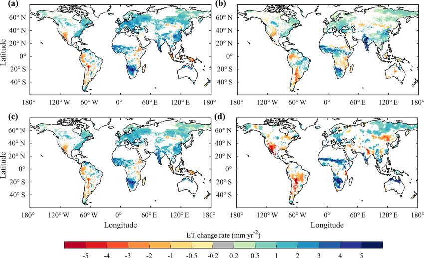
1488                                                                         S. Pan et al.: Evaluation of global terrestrial ET

where fstress is a stress factor and is usually computed as a     algorithms, such as those based on artificial neural networks,
function of environmental conditions. α is the PT param-          random forest, and support vector machine algorithms, have
eter with a value of between 1.2 and 1.3 under water un-          been applied in various ecosystems (Antonopoulos et al.,
stressed conditions and can be estimated using remote sens-       2016; Chen et al., 2014; Feng et al., 2017; Shrestha and
ing. Although the original PT equation works well for es-         Shukla, 2015) and have proved to be more accurate in es-
timating potential ET across most surfaces, the Priestley–        timating ET than simple regression models (Antonopoulos
Taylor coefficient, α, usually needs adjustment to convert        et al., 2016; Chen et al., 2014; Kisi et al., 2015; Shrestha and
potential ET to actual ET (K. Zhang et al., 2016). Thus,          Shukla, 2015; Tabari et al., 2013). In upscaling FLUXNET
Fisher et al. (2008) developed a modified PT model that           ET to the global scale, Jung et al. (2010) used the model
keeps α constant but scales down potential ET using eco-          tree ensemble method to integrate eddy-covariance measure-
physiological constraints and soil evaporation partitioning.      ments of ET with satellite remote sensing and surface mete-
The accuracy of their model has been validated against eddy-      orological data. In a recent study (Bodesheim et al., 2018),
covariance measurements conducted in a wide range of cli-         the random forest approach was used to derive global ET at
mates and involving many plant functional types (Fisher et        a 30 min timescale.
al., 2009; Vinukollu et al., 2011b). Following this idea, Yao
et al. (2013) further developed a modified Priestley–Taylor       2.1.3    Process-based land surface models (LSMs)
algorithm that constrains soil evaporation using the index
of the soil water deficit derived from the apparent thermal       Although satellite-derived ET products have provided quan-
inertia. Miralles et al. (2011) also proposed a novel PT-         titative investigations of historical terrestrial ET dynamics,
type model: the Global Land Evaporation Amsterdam Model           they can only cover a limited temporal record of about 4
(GLEAM). GLEAM combines a soil water module, a canopy             decades. To obtain terrestrial ET before the 1980s and pre-
interception model and a stress module within the PT equa-        dict future ET dynamics, LSMs are needed, as they are able
tion. The key distinguishing features of this model are the       to represent a large number of interactions and feedbacks
use of microwave-derived soil moisture, land surface tem-         between physical, biological and biogeochemical processes
perature and vegetation density, and the detailed estimation      in a prognostic way (Jimenez et al., 2011). ET simulation
of rainfall interception loss. In this way, GLEAM minimizes       in LSMs is regulated by multiple biophysical and physio-
the dependence on static variables, avoids the need for pa-       logical properties or processes, including but not limited to
rameter tuning and enables the quality of the evaporation es-     stomatal conductance, leaf area, root water uptake, soil wa-
timates to rely on the accuracy of the satellite inputs (Mi-      ter, runoff and (sometimes) nutrient uptake (Famiglietti and
ralles et al., 2011). Compared with the PM approach, the          Wood, 1991; Huang et al., 2016; Lawrence et al., 2007). Al-
PT-based approaches avoid the computational complexities          though almost all current LSMs have these components, dif-
of aerodynamic resistance and the accompanying error prop-        ferent parameterization schemes result in substantial differ-
agation. However, the many simplifications and semiempir-         ences in ET estimation (Wartenburger et al., 2018). There-
ical parameterization of physical processes in the PT-based       fore, in recent years, the multi-model ensemble approach has
approaches may lower its accuracy.                                become popular in quantifying the magnitude, spatiotempo-
                                                                  ral pattern and uncertainty of global terrestrial ET (Mueller
2.1.2   Vegetation-index-based empirical algorithms and           et al., 2011; Wartenburger et al., 2018). Yao et al. (2017)
        machine-learning methods                                  showed that a simple model averaging method or a Bayesian
                                                                  model averaging method is superior to each individual model
The principle of empirical ET algorithms is to link observed      in predicting terrestrial ET.
ET to its controlling environmental factors through various
statistical regressions or machine-learning algorithms of dif-    2.2     Description of ET models used in this study
ferent complexities. The earliest empirical regression method
was proposed by Jackson et al. (1977). At present, the ma-        In this study, we evaluate 20 ET products that are based on
jority of regression models are based on vegetation indices       remote-sensing-based physical models, machine-learning al-
(Glenn et al., 2010), such as the NDVI and the enhanced veg-      gorithms and LSMs to investigate the magnitudes and spatial
etation index (EVI), because of their simplicity, resilience in   patterns of global terrestrial ET over recent decades. Table 1
the presence of data gaps, utility under a wide range of con-     lists the input data, the ET algorithms adopted, the advan-
ditions and connection with vegetation transpiration capacity     tages and limitations, and the references for each product.
(Maselli et al., 2014; Nagler et al., 2005; Yuan et al., 2010).   We use a simple model averaging method when calculating
As an alternative to statistical regression methods, machine-     the mean value of multiple models.
learning algorithms have been gaining increased attention for        Four physically based remote sensing datasets, includ-
ET estimation due to their ability to capture the complex non-    ing the Process-based Land Surface Evapotranspiration/Heat
linear relationships between ET and its controlling factors       Fluxes algorithm (P-LSH), the Global Land Evaporation
(Dou and Yang, 2018). Many conventional machine-learning          Amsterdam Model (GLEAM), the Moderate Resolution

Hydrol. Earth Syst. Sci., 24, 1485–1509, 2020                                    www.hydrol-earth-syst-sci.net/24/1485/2020/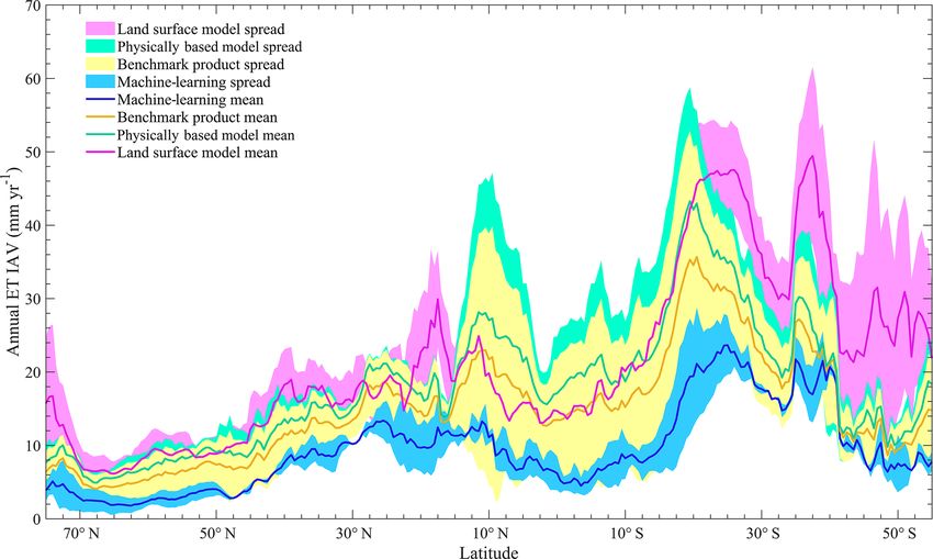
Table 1. Descriptions of the models used in this study, including their drivers, adopted algorithms, key equations, advantages and limitations, and references.
Name Input Algorithm Spatial Temporal Key equations Advantages and limitations References
resolution resolution
MTE Climate: precipitation, tem- TRIAL + 0.5◦ × 0.5◦ Monthly No specific equation Limitations: insufficient flux observations Jung et al.
perature, sunshine hour, rel- ERROR in tropical regions; no CO2 effect (2011)
ative humidity and wet days
Vegetation: fAPAR
RF Climate: land surface Randomized 0.5◦ × 0.5◦ 30 min No specific equation Limitations: the same as for MTE Bodesheim
temperature, radiation, decision tree et al. (2018)
potential radiation,
index of water availability
and relative humidity
Vegetation: fAPAR ,
LAI and enhanced
vegetation index (EVI)
1Rn +ρCp VPDga
P-LSH Climate: radiation, air tem- Modified 0.083◦ × 0.083◦ Monthly Ev = Advantages: more robust physical basis; Zhang et al.
www.hydrol-earth-syst-sci.net/24/1485/2020/
λv 1+ϒ 1+ ggas
perature, vapor pressure, Penman– considers the effects of CO2 (2015)
VPD 1Rn +ρCp VPDga
wind speed and CO2 Monteith k Limitations: high meteorological forcing
S. Pan et al.: Evaluation of global terrestrial ET
Es = RH
Vegetation: AVHRR NDVI λv 1+ϒ 1+ ggas requirements; canopy conductance is based
on proxies
GLEAM Climate: precipitation, net Modified 0.25◦ × 0.25◦ Daily E s = fs Ss α s λ ρ 1 Rns − Gs Advantages: simple; low requirement for Miralles et
v w (1+γ )
radiation, surface soil Priestley– Esc = fsc Ssc αsc λ ρ 1 Rnsc − Gsc meteorological data; well-suited for remote al. (2011)
moisture, land surface Taylor v w (1+γ ) sensing observable variables; soil moisture
Etc = ftc Stc αtc λ ρ 1 tc
temperature, air tempera- v w (1+γ ) Rn − Gtc − βEi is considered
ture and snow depth Limitations: many simplifications of physi-
Vegetation: vegetation opti- cal processes; neither VPD nor surface and
cal depth aerodynamic resistances are explicitly
accounted for; strong dependency on net
radiation
1(Rn −G)+ρcp VPD
rawc
MODIS Climate: air temperature, Penman– 0.05◦ × 0.05◦ Monthly Ei = fwet fc
r wc
Advantages: more robust physical basis; Mu et al.
shortwave radiation, wind Monteith– λv ρw 1+γ rswc Limitations: requires many variables that (2011)
a
speed, relative humidity Leuning 1(Rn −G)+ρcp VPD are difficult to observe or that are not ob-
rat
and air pressure Ev = (1 − fwet ) fc
servable with satellites; canopy conduc-
rst
λv ρw 1+ϒ t
Vegetation: LAI and r tance is based on
a
fAPAR , albedo h i sAsoil + ρcp (1−fc )VPD
ras
proxies; does not consider soil moisture but
(1−fwet )hVPD
Es = fwet + β
uses atmospheric humidity as a surrogate;
λ ρ S+γ rtot
v w ras
does not consider the effects of CO2
1Rn +ρCp VPDga
PML- Climate: precipitation, air Penman– 0.5◦ × 0.5◦ Monthly Ev = Advantages: more robust physical basis Y. Zhang et
λv 1+ϒ 1+ ggas
CSIRO temperature, vapor pres- Monteith– (compared with Priestley–Taylor equa- al. (2016)
1As
sure, shortwave radiation, Leuning Es = f1+γ tion);
longwave radiation and Ei : an adapted version of the Gash rainfall intercep- biophysically based estimation of surface
wind speed tion model (Van Dijk and Bruijnzeel, 2001) conductance
Vegetation: AVHRR LAI, Limitations: high meteorological forcing
emissivity and albedo requirements; canopy conductance is based
on proxies; does not consider the effects of
CO2
Hydrol. Earth Syst. Sci., 24, 1485–1509, 2020
1489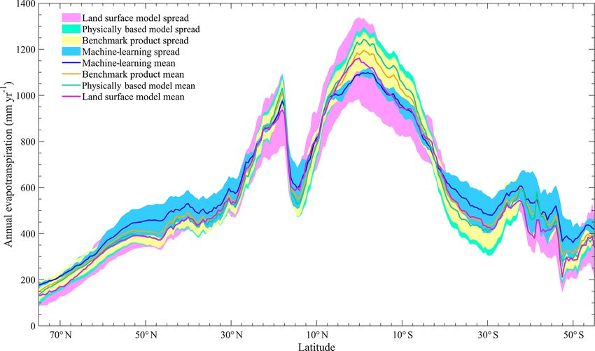
Table 1. Continued.
S. Pan et al.: Evaluation of global terrestrial ET
www.hydrol-earth-syst-sci.net/24/1485/2020/
TRENDY LSMs
Advantages: land surface models are process-oriented and physically based. Given their structure almost all models are capable of allowing factorial analysis, where one forcing can be applied at a time. Most models also consider
the physiological effect of CO2 on stomatal closure.
Limitations: most models typically do not allow integration/assimilation of observation-based vegetation characteristics. Model parameterizations remain uncertain and the same process is modeled in different ways across
models. Model parameters may or may not be physically based and, therefore, measurable in the field.
Models participating in the TRENDYv6 comparison were forced by precipitation, air temperature, specific humidity, shortwave radiation, longwave radiation and wind speed based on the CRU-NCEPv8 data, as explained in Le Quéré
et al. (2018). It is very difficult to list all key equations for all land surface models. Thus, we only list the stomatal conductance equation for each model in this table.
Name Algorithm Spatial Temporal Key equations References
resolution resolution
VPD −1
CABLE Penman–Monteith 0.5◦ × 0.5◦ Monthly gs = g0 + gc1af−c
wA
p
1 + VPD Haverd et al. (2018)
0
CLASS- Modified Penman–Monteith 2.8125◦ × 2.8125◦ Monthly gc = m (cA−0)
np 1
(1+VPD/VPD0 ) + b LAI Melton and Arora (2016)
s
CTEM
CLM45 Modified Penman–Monteith 1.875◦ × 2.5◦ Monthly gs = g0 + gc1aA RH Oleson et al. (2010)
DLEM Penman–Monteith 0.5◦ × 0.5◦ Monthly gs = max (gsmax rcorr bf (ppdf) f (Tmin ) f (VPD) f (CO2 ) , gsmin ) Pan et al. (2015)
ISAM Modified Penman–Monteith 0.5◦ × 0.5◦ Monthly A
gs = m C /P × eesi + bt βt Barman et al. (2014)
s atm
1.6A
JSBACH Penman–Monteith 1.9◦ × 1.9◦ Monthly gs = βw ca −cn,pot
i,pot
Knauer et al. (2015)
1 θ1 2
JULES Penman–Monteith 2.5◦ × 3.75◦ Monthly Bare soil conductance: gsoil = 100 θc Li et al. (2016)
Stomatal conductance is calculated by solving the following two
equations:
Ci −0 ∗
1
Al = gs (Cs − Ci ) /1.6; C ∗ = f0 1 − q
c −0 c
LPJ- Equations proposed by Monteith (1995) 0.5◦ × 0.5◦ Monthly gs = gsmin + c 1.6Adt
(1−λ ) Smith (2001)
a c
GUESS
LPJ-wsl Priestley–Taylor 0.5◦ × 0.5◦ Monthly gs = gsmin + c 1.6Adt Sitch et al. (2003)
a (1−λc )
LPX-Bern Modified equation of Monteith (1995) 1◦ × 1◦ Monthly gs = gsmin + c 1.6Adt Keller et al. (2017)
a (1−λc )
gs = gsmin + c 1.6A
Hydrol. Earth Syst. Sci., 24, 1485–1509, 2020
O-CN Modified Penman–Monteith 1◦ × 1◦ Monthly dt Zaehle and Friend (2010)
a (1−λc )
ORCHIDEE Modified Penman–Monteith 0.5◦ × 0.5◦ Monthly gs = g0 + A+R d
ca −cp fvpd d’Orgeval et al. (2008)
gsoil = exp (8.206 − 4.255W/Wsat )
ORCHIDEE- Modified Penman–Monteith 0.5◦ × 0.5◦ Monthly gs = g0 + A+R d
ca −cp fvpd Guimberteau et al. (2018)
MICT
VPD −1
VISIT Penman–Monteith 0.5◦ × 0.5◦ Monthly gs = g0 + gc1af−c
wA
p
1 + VPD Ito (2010)
0
Notes: A: net assimilation rate; Adt : total daytime net photosynthesis; An,pot : unstressed net assimilation rate; b: soil moisture factor; bt : stomatal conductance intercept; ca : atmospheric CO2 concentration; cc : critical CO2 concentration;
ci : internal leaf concentration of CO2 ; ci,pot : internal leaf concentration of CO2 for unstressed conditions; cs : leaf surface CO2 concentration; cp : CO2 compensation point; es : vapor pressure at leaf surface; ei : saturation vapor pressure
inside the leaf; Es : soil evaporation; Ec : canopy evapotranspiration; Edry : dry canopy evapotranspiration; Ewet : wet canopy evapotranspiration; Ev : canopy transpiration; Ei : canopy interception; Etc : transpiration from tall canopy;
Esc : transpiration from short canopy; f : fraction of P to equilibrium soil evaporation; fs : soil fraction; fsc : short canopy fraction; ftc : tall canopy fraction; fvpd : factor of the effect of leaf-to-air vapor pressure difference; fw : a function
describing the soil water stress on stomatal conductance; fwet : relative surface wetness parameter; f0 : the maximum ratio of internal to external CO2 ; f (ppdf):limiting factor of photosynthetic photo flux density; f (Tmin ): limiting factor
of daily minimum temperature; f (VPD): limiting factor of vapor pressure deficit; f (CO2 ): limiting factor of carbon dioxide; G: ground energy flux; ga : aerodynamic conductance; gm : empirical parameter; gs : stomatal conductance;
gsmax : maximum stomatal conductance; gsmin : minimum stomatal conductance; gsoil : bare soil conductance; g0 : residual stomatal conductance when the net assimilation rate is 0 ; g1 : sensitivity of stomatal conductance to assimilation,
ambient CO2 concentration and environmental controls; I : tall canopy interception loss; m: stomatal conductance slope; Patm : atmospheric pressure; PEs : potential soil evaporation; PEcanopy : potential canopy evaporation; qa : specific air
humidity; qc : critical humidity deficit; qs : specific humidity of saturated air; ra : aerodynamic resistance; rs : stomatal resistance; Rn : net radiation; Rd: day respiration; RH: relative humidity; Ts : actual surface temperature; VPD: vapor
pressure deficit; VPD0 : the sensitivity of stomatal conductance to VPD; W : top soil moisture; Wcanopy : canopy water; Wsat : soil porosity; α : Priestley–Taylor coefficient; αm : empirical parameter; β : a constant accounting for the times
when vegetation is wet; βt : soil water availability factor between 0 and 1; βw : a scaling factor to account for water stress; βs : moisture availability function; ρ : air density; γ : psychrometric constant; λv : latent heat of vaporization;
1490
λc : ratio of intercellular to ambient partial pressure of CO2 ; rcorr : correction factor of temperature and air pressure on conductance; 0 ∗ : CO2 compensation point when leaf day respiration is zero; θ1 : parameter of moisture concentration
in the top soil layer; θc : parameter of moisture concentration in the spatially varying critical soil moisture; 1: slope of the vapor pressure curve.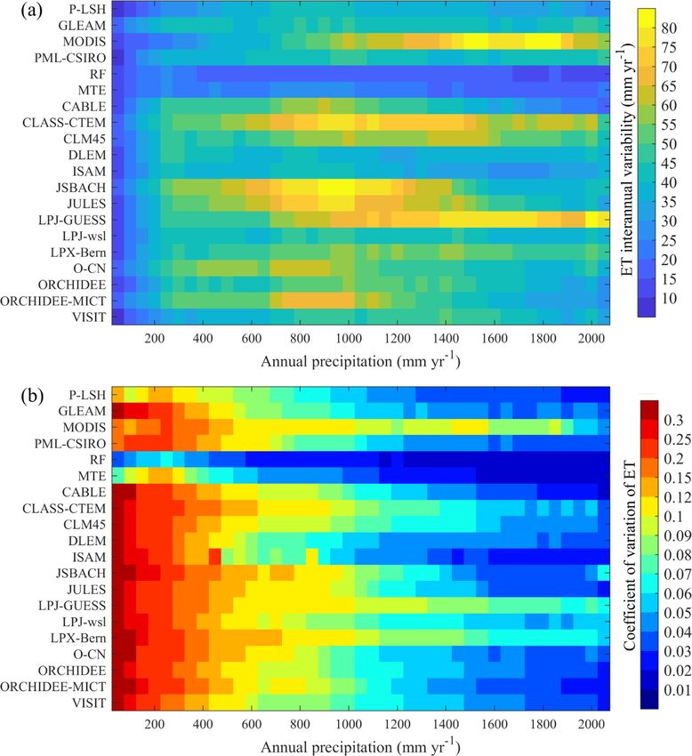
S. Pan et al.: Evaluation of global terrestrial ET                                                                          1491

Imaging Spectroradiometer (MODIS) and the PML-CSIRO                2009). The TRIAL grows model trees from the root node and
(Penman–Monteith–Leuning), and two machine-learning                splits at each node with the criterion of minimizing the sum
datasets, which are based on random forest (RF) and model          of squared errors of multiple regressions in both subdomains.
tree ensemble (MTE), are used in our study. Both machine-          ERROR is used to select the model trees that are indepen-
learning and physically based remote sensing datasets (six         dent of one another and have the best performance based on
datasets in total) were considered as benchmark products.          the Schwarz criterion. The canopy fraction of absorbed pho-
The ensemble mean of the benchmark products was calcu-             tosynthetic active radiation (fAPAR ), temperature, precipita-
lated as the mean value of all machine-learning and physi-         tion, relative humidity, sunshine hours and potential radia-
cally based satellite estimates as we treated each benchmark       tion are used as explanatory variables to train MTE (Jung et
dataset equally.                                                   al., 2011). The second machine-learning model is the random
   Three of the four remote-sensing-based physical models          forest (RF) algorithm, whose rationale is generating a set of
quantify ET using PM approaches. P-LSH adopts a modified           independent regression trees by randomly selecting training
PM approach coupled with biome-specific canopy conduc-             samples automatically (Breiman, 2001). Each regression tree
tance determined from NDVI (Zhang et al., 2010). The mod-          is constructed using samples selected by a bootstrap sam-
ified P-LSH model used in this study also accounts for the in-     pling method. After fixing the individual tree in entity, the
fluences of atmospheric CO2 concentrations and wind speed          final result is determined by simple averaging. One merit of
on canopy stomatal conductance and aerodynamic conduc-             the RF algorithm is its capability to handle complicated non-
tance (Zhang et al., 2015). The MODIS ET model is based            linear problems and high dimensional data (Xu et al., 2018).
on the algorithm proposed by Cleugh et al. (2007). Mu et           For the RF product used in this study, multiple explanatory
al. (2007) improved the model performance through the in-          variables including the enhanced vegetation index, fAPAR ,
clusion of environmental stress into the canopy conductance        the leaf area index, daytime and nighttime land surface tem-
calculation and by explicitly accounting for soil evaporation      perature, incoming radiation, top-of-atmosphere potential ra-
by combining the complementary relationship hypothesis             diation, the index of water availability and relative humidity
with the PM equation. The MODIS ET product (MOD16A3)               were used to train regression trees (Bodesheim et al., 2018).
used in this study was further improved by considering night-         The 14 LSM-derived ET products were from the Trends
time ET, simplifying the vegetation cover fraction calcula-        and Drivers of the Regional Scale Sources and Sinks
tion, adding the soil heat flux item, dividing the saturated wet   of Carbon Dioxide (TRENDY) project (including CA-
and moist soil, separating the dry and wet canopy, as well         BLE, CLASS-CTEM, CLM45, DLEM, ISAM, JSBACH,
as modifying algorithms of aerodynamic resistance, stom-           JULES, LPJ-GUESS, LPJ-wsl, LPX-Bern, O-CN, OR-
atal conductance and boundary layer resistance (Mu et al.,         CHIDEE, ORCHIDEE-MICT and VISIT). Daily gridded
2011). PML-CSIRO adopts the Penman–Monteith–Leuning                meteorological reanalyzes from the CRU-NCEPv8 dataset
algorithm, which calculates surface conductance and canopy         (temperature, precipitation, long- and shortwave incoming
conductance using a biophysical model instead of classic em-       radiation, wind speed, humidity and air pressure) were used
pirical models. The maximum stomatal conductance is es-            to drive the LSMs. The TRENDY simulations were per-
timated using the trial-and-error method (Y. Zhang et al.,         formed in year 2017 and contributed to the global carbon
2016). Furthermore, for each grid covered by natural veg-          budget reported in Le Quéré et al. (2018). We used the re-
etation, the PML-CSIRO model constrains ET at the annual           sults from the S3 simulation from TRENDYv6 (with chang-
scale using the Budyko hydrometeorological model proposed          ing CO2 , climate and land use) over the period from 1982
by Fu (1981). The GLEAM ET calculation is based on the             to 2011, which is a time period consistent with other prod-
PT equation, which requires fewer model inputs than the            ucts derived from remote-sensing-based physical models and
PM equation, and the majority of these inputs can be di-           machine-learning algorithms.
rectly achieved from satellite observations. Its rationale is to
make the most of information about evaporation contained in        2.3   Description of other datasets
the satellite-based environmental and climatic observations
(Martens et al., 2017; Miralles et al., 2011). Key variables       To quantify the contributions of vegetation greening to terres-
including air temperature, land surface temperature, precipi-      trial ET variations, we used the LAI from the TRENDYv6
tation, soil moisture, vegetation optical depth and snow water     S3 simulation. We also used the newest version of the
equivalent are satellite-observed values. Moreover, the exten-     Global Inventory Modeling and Mapping Studies LAI data
sive usage of microwave remote sensing products in GLEAM           (GIMMS LAI3gV1) as the satellite-derived LAI. GIMMS
ensures the accurate estimation of ET under diverse weather        LAI3gV1 was generated from AVHRR GIMMS NDVI3g us-
conditions. Here, we use GLEAM v3.2, which has overall             ing a model derived from an artificial neural network (ANN;
better quality than previous versions (Martens et al., 2017).      Zhu et al., 2013). It covers the period from 1982 to 2016
   The first used machine-learning model, MTE, is based            with bimonthly frequency and has a 1/12◦ spatial resolu-
on the Tree Induction Algorithm (TRIAL) and Evolving               tion. To achieve a uniform resolution, all data were resam-
Trees with Random Growth (ERROR) algorithm (Jung et al.,           pled to 1/2◦ using the nearest neighbor method. Follow-

www.hydrol-earth-syst-sci.net/24/1485/2020/                                     Hydrol. Earth Syst. Sci., 24, 1485–1509, 2020
1492                                                                           S. Pan et al.: Evaluation of global terrestrial ET

ing N. Pan et al. (2018), grids with an annual mean NDVI                                  LAI , γ T , γ P and γ R , the contribu-
                                                                       After calculating γET     ET    ET      ET
of less than 0.1 were assumed to be non-vegetated regions           tion of the trend in factor i (Trend(i)) to the trend in ET
and were, therefore, masked out. NDVI data are from the             (Trend(ET)) can be quantified as follows:
GIMMS NDVI3gV1 dataset. Temperature, precipitation and
                                                                                   i
radiation are from the CRU-NCEPv8 dataset.                          Contri(i) = γET   × Trend (i) /Trend(ET).                 (5)

2.4    Statistical analysis                                         In performing multiple linear regression, we used the
                                                                    GIMMS LAI for both remote-sensing-based physical mod-
The significance of ET trends was analyzed using the Mann-          els and machine-learning methods as well as the individ-
Kendall (MK) test (Kendall, 1955; Mann, 1945). It is a rank-        ual TRENDYv6 LAI for each TRENDY model. The grid-
based nonparametric method that has been widely applied             ded data of temperature, precipitation and radiation are from
for detecting trends in hydro-climatic time series (Sayemuz-        CRU-NCEPv8.
zaman and Jha, 2014; Yue et al., 2002). The Theil–Sen es-
timator was applied to estimate the magnitude of the slope.
The advantage of this method over an ordinary least squares         3     Results
estimator is that it limits the influence of the outliers on the
slope (Sen, 1968).                                                  3.1    The ET magnitude estimated by multiple models
   Terrestrial ET interannual variability (IAV) is mainly con-
trolled by variations in temperature, precipitation and short-      The multiyear ensemble mean of annual global terrestrial ET
wave solar radiation (Zeng et al., 2018b; Zhang et al., 2015).      from 2001 to 2011 derived by machine-learning methods,
In this study, we performed partial correlation analyses be-        remote-sensing-based physical models and the TRENDY
tween ET and these three climatic variables at an annual            models agreed well, with values ranging from 589.6 to
scale for each grid cell to explore climatic controls on ET         617.1 mm yr−1 . However, substantial differences existed
IAV. Variability caused by climatic variables was assessed          among individual models (Fig. 1). LPJ-wsl (455.3 mm yr−1 )
through the square of partial correlation coefficients between      and LPX-Bern (453.7 mm yr−1 ) estimated significantly
ET and temperature, precipitation and radiation. We chose           lower ET than other models, even in comparison with most
partial correlation analysis because it can quantify the link-      previous studies focusing on earlier periods (Table S1 in
age between ET and a single environmental driving factor            the Supplement). On the contrary, JULES gave the largest
while controlling the effects of the other remaining environ-       ET estimate (697.3 mm yr−1 , which is equal to 7.57 ×
mental factors. Partial correlation analysis is a widely ap-        104 km3 yr−1 ) among all models, and showed an obvious in-
plied statistical tool to isolate the relationship between two      crease in ET compared with its estimation from 1950 to 2000
variables from the confounding effects of many correlated           (6.5 × 10⁴ km3 yr−1 , Table S1).
variables (Anav et al., 2015; Jung et al., 2017; Peng et al.,
                                                                    3.2    Spatial patterns of global terrestrial ET
2013). All variables were first detrended in the statistical cor-
relation analysis, as we focus on the interannual relationship.     As shown in Fig. 2, the spatial patterns of the multiyear
The study period is from 1982 to 2011 for all models except         average annual ET of different categories were similar. ET
MODIS and random forest, which have a temporal coverage             was highest in the tropics and low in the northern high lat-
that is limited to 2001–2011 because of data availability.          itudes and arid regions such as Australia, central Asia, the
   To quantify the contribution of vegetation greening to ter-      western US and the Sahel. Compared with remote-sensing-
restrial ET, we separated the trend in terrestrial ET into four     based physical models and LSMs, machine-learning meth-
components induced by climatic variables and vegetation dy-         ods obtained a smaller spatial gradient. In general, latitudi-
namics by establishing a multiple linear regression model be-       nal profiles of ET estimated using different approaches were
tween global ET and temperature, precipitation, shortwave           also consistent (Fig. 3). However, machine-learning meth-
radiation and LAI (Eqs. 3, 4):                                      ods gave higher ET estimate at high latitudes and lower ET
                                                                    in the tropics compared with other approaches. In the trop-
          ∂ (ET)            ∂ (ET)         ∂ (ET)
δ (ET) =          δ (LAI) +        δ (T) +        δ (P )            ics, LSMs have significantly larger uncertainties than bench-
         ∂ (LAI)              ∂T           ∂ (P )                   mark products, and the standard deviation of LSMs is about
         ∂ (ET)                                                     2 times higher than that of benchmark products (Fig. 3). At
       +        δ (R) + ε                                (3)
           ∂R                                                       other latitudes, LSMs and benchmark ET products generally
           LAI          T        P            R                     have comparable uncertainties. The largest difference in ET
δ (ET) = γET   δLAI + γET δT + γET  δP + +γET   δR + ε, (4)
                                                                    in the different categories was found in the Amazon Basin
where γETLAI , γ T , γ P and γ R are the sensitivities of ET to     (Fig. 2). In most regions of the Amazon Basin, the mean ET
                ET ET         ET
the leaf area index (LAI), air temperature (T ), precipitation      of remote sensing physical models is more than 200 mm yr−1
(P ) and radiation (R), respectively. ε is the residual, repre-     higher than the mean ET of LSMs and machine-learning
senting the impacts of other factors.                               methods. For individual ET estimates, the largest uncertainty

Hydrol. Earth Syst. Sci., 24, 1485–1509, 2020                                       www.hydrol-earth-syst-sci.net/24/1485/2020/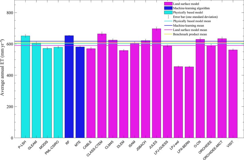
S. Pan et al.: Evaluation of global terrestrial ET 1493
Figure 1. Average annual global terrestrial ET estimated by each model during the period from 2001 to 2011. Error bars represent the
standard deviation of each model. The four lines indicate the mean value of each category.
was also found in the Amazon Basin. MODIS, VISIT and contrast, the IAV of machine-learning-based ET was much
CLASS-CTEM estimated that the annual ET was higher weaker. In most regions, the IAV of machine-learning ET is
than 1300 mm in the majority of Amazon, whereas JSBACH lower than 40 % of the IAV of remote sensing physical ET
and LPJ-wsl estimated an ET value lower than 800 mm yr−1 and LSM ET, and this phenomenon is especially pronounced
(Fig. S1). As is shown in Fig. S2, the differences in ET in tropical regions. Further investigation into the spatial pat-
estimates among TRENDY models were larger than those terns of ET IAV for individual models showed that the two
among benchmark estimates for tropical and humid regions. machine-learning methods performed equally with respect
The uncertainty of ET estimates from LSMs is particularly to estimating spatial patterns of ET IAV (Fig. S4). In con-
large in the Amazon Basin, where the standard deviation of trast, differences in ET IAV among remote sensing physi-
LSM estimates is more than 2 times larger than that of bench- cal estimates and LSM estimates were much larger. LSMs
mark estimates. It is noteworthy that, in arid and semiarid re- showed the largest differences in the IAV of ET in tropical
gions such as western Australia, central Asia, northern China regions. For example, CABLE and JULES obtained an ET
and the western US, the difference in ET estimates among IAV of less than 15 mm yr−1 in most regions of the Amazon
LSMs is significantly smaller than those among remote sens- Basin, whereas LPJ-GUESS predicted an ET IAV of more
ing models and machine-learning algorithms. than 60 mm yr−1 . Figure 5 shows that remote sensing physi-
cal ET and LSM ET had comparable IAV north of 20◦ S, but
3.3 Interannual variations in global terrestrial ET the IAV of the machine-learning-based ET was much lower
in this region. In the region south of 20◦ S, TRENDY ET
showed the largest IAV, followed by those of remote sensing
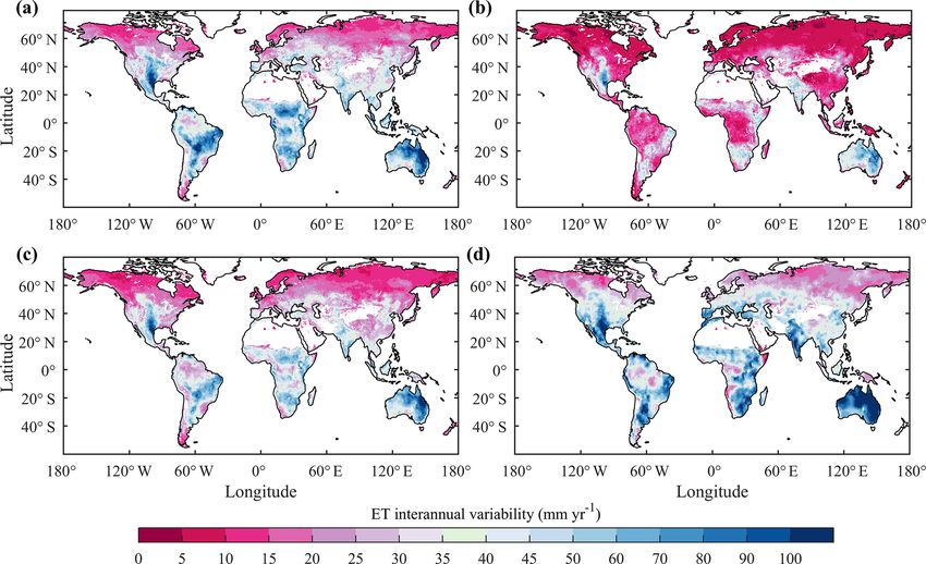
The ensemble mean interannual variability (IAV) of remote
physical ET and machine-learning estimates. The three ap-
sensing ET estimates and LSM ET estimates showed sim-
proaches agreed on that ET IAV in the Southern Hemisphere
ilar spatial patterns (Fig. 4). Both remote sensing physical
was generally larger than that in the Northern Hemisphere.
models and LSMs presented low IAV in ET in the north-
ern high latitudes but high IAV in ET in the southwestern
US, India, sub-Saharan Africa, the Amazon and Australia. In
www.hydrol-earth-syst-sci.net/24/1485/2020/ Hydrol. Earth Syst. Sci., 24, 1485–1509, 20201494 S. Pan et al.: Evaluation of global terrestrial ET Figure 2. Spatial distributions of the mean annual ET derived from (a) remote-sensing-based physical models, (b) machine-learning algo- rithms, (c) benchmark datasets and (d) the TRENDY LSMs’ ensemble mean, respectively. Figure 3. Latitudinal profiles of the mean annual ET for different categories of models. Each line represents the mean value of the corre- sponding category, and the shading represents the interval of 1 standard deviation. Hydrol. Earth Syst. Sci., 24, 1485–1509, 2020 www.hydrol-earth-syst-sci.net/24/1485/2020/
S. Pan et al.: Evaluation of global terrestrial ET                                                                                       1495

Figure 4. Spatial distributions of the interannual variability in ET derived from (a) remote-sensing-based physical models, (b) machine-
learning algorithms, (c) benchmark datasets and (d) the TRENDY LSMs’ ensemble mean, respectively. The study period used in this study
for the interannual variability analysis is from 1982 to 2011.

Figure 5. Latitudinal profiles of ET IAV for different categories of models. Each line represents the mean value of the corresponding category,
and the shading represents the interval of 1 standard deviation.

www.hydrol-earth-syst-sci.net/24/1485/2020/                                             Hydrol. Earth Syst. Sci., 24, 1485–1509, 2020
1496 S. Pan et al.: Evaluation of global terrestrial ET
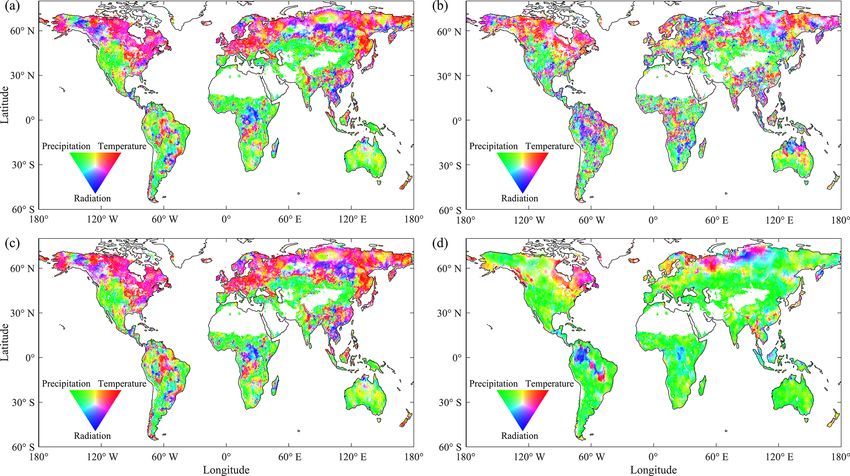
3.4 Climatic controls on ET All remote sensing and machine-learning estimates indi-
cate a significant increasing trend in ET during the study
According to the ensemble remote sensing models, temper- period (p < 0.05), although the increase rate of P-LSH
ature and radiation dominated ET IAV in northern Eura- (1.07 mm yr−2 ) is more than 3 times as large as that of
sia, northern and eastern North America, southern China, GLEAM (0.33 mm yr−2 ). Nevertheless, there is a larger dis-
the Congo River basin, and the southern Amazon River crepancy among LSMs in terms of the ET trend. The ma-
basin, while precipitation dominated ET IAV in arid re- jority of LSMs (10 of 14) suggest an increasing trend
gions and semiarid regions (Fig. 6a). The ensemble machine- with an average trend of 0.34 mm yr−2 (p < 0.05), and
learning algorithms had a similar pattern, but they suggested eight of them are statistically significant (see Table 2).
a stronger control of radiation in the Amazon Basin and a However, four LSMs (JSBACH, JULES, ORCHIDEE and
weaker control of precipitation in several arid regions such ORCHIDEE-MICT) suggest a decreasing trend with an av-
as central Asia and northern Australia (Fig. 6b). In com- erage trend of −0.12 mm yr−2 (p > 0.05). Among the four
parison, the ensemble LSMs suggested the strongest control decreasing trends, only the trend of ORCHIDEE-MICT
of precipitation on ET IAV (Fig. 6). According to the en- (−0.34 mm yr−2 ) is statistically significant (p < 0.05).
semble LSMs, ET IAV was dominated by precipitation IAV According to Fig. 8, the ensemble means of all the three
in most regions of the Southern Hemisphere and at north- approaches showed increasing trends in ET over western and
ern low latitudes. Temperature and radiation only controlled southern Africa, western India and northern Australia, and
northern Eurasia, eastern Canada and part of the Amazon decreasing ET over the western US, southern South Amer-
Basin (Fig. 6d). As is shown in Fig. S6, the majority of ica and Mongolia. Discrepancies in ET trends mainly ap-
LSMs agreed on the dominant role of precipitation in con- peared in eastern Europe, eastern India and central China.
trolling ET in regions south of 40◦ N. However, the pattern LSMs also suggested a larger area of decreasing ET in both
of climatic controls in the ORCHIDEE-MICT model is quite North America and South America. Although the differences
unique and different from all of the other LSMs. Accord- in ET trends among individual models were larger than those
ing to the ORCHIDEE-MICT model, radiation and temper- among the ensemble means of different approaches, the ma-
ature dominate ET IAV in more regions, and precipitation jority of models agreed that ET increased in western and
only controls ET IAV in eastern Brazil, northern Russia, cen- southern Africa, and decreased in the western US and south-
tral Europe and a part of tropical Africa. As ORCHIDEE- ern South America (Fig. S2). For both remote sensing esti-
MICT was developed from ORCHIDEE, the dynamic root mates and LSM estimates, ET trends in the Amazon Basin
parameterization in ORCHIDEE-MICT may explain why ET had large uncertainty: P-LSH, CLM45 and VISIT suggested
is less driven by precipitation compared with ORCHIDEE a large area of increasing ET, whereas GLEAM, JSBACH
(Haverd et al., 2018). It is noted that two machine-learning and ORCHIDEE suggested a large area of decreasing ET.
algorithms, MTE and RF, showed significant discrepancies
in the spatial pattern of dominant climatic factors. Accord- 3.6 Impacts of vegetation changes on ET variations
ing to the result from MTE, temperature controlled ET IAV
in regions north of 45◦ N, the eastern US, southern China During the period from 1982 to 2011, global LAI trends es-
and the Amazon Basin (Fig. S6e). By contrast, RF suggested timated from remote sensing data and from the ensemble
that precipitation and radiation dominated ET IAV in these LSMs are 2.51 × 10⁻³ m2 m−2 yr−1 (p < 0.01) and 4.63 ×
regions (Fig. S6f). 10−3 m2 m−2 yr−1 (p < 0.01), respectively (Table 2). All
LSMs suggested a significant increasing trend in global
3.5 Long-term trends in global terrestrial ET LAI (greening). For both benchmark estimates and LSM
estimates, it was found that the spatial pattern of trends
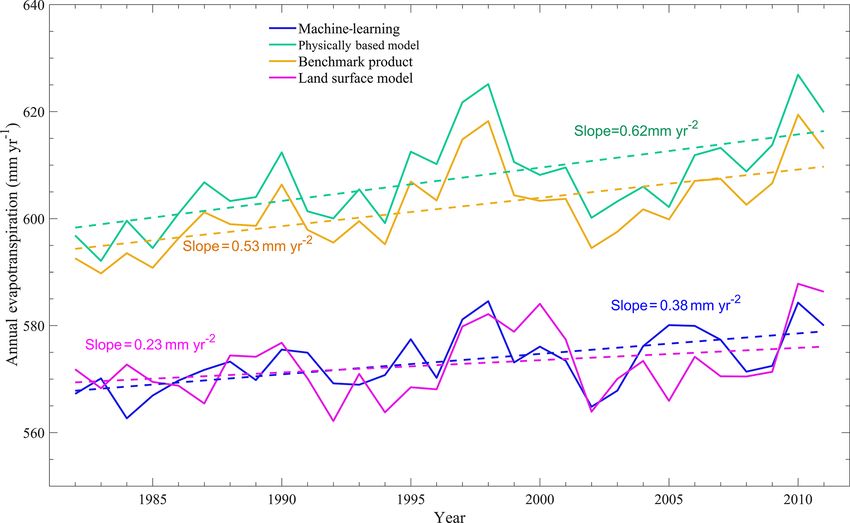
All approaches suggested an overall increasing trend in
in ET matched well with that of trends in the LAI
global ET during the period from 1982 to 2011 (Fig. 7), al-
(Figs. 8c, d, S5a, b), indicating significant effects of veg-
though ET decreased from 1998 to 2009. This result is con-
etation dynamics on ET variations. According to the re-
sistent with previous studies (Jung et al., 2010; Lian et al.,
sults of the multiple linear regression, all models agreed
2018; Zhang et al., 2015). Remote sensing physical mod-
that greening of the Earth since the early 1980s intensified
els indicated the largest increase in ET (0.62 mm yr−2 ), fol-
terrestrial ET (Table 2), although there was a significant
lowed by the machine-learning method (0.38 mm yr−2 ) and
discrepancy in the magnitude of ET intensification which
land surface models (0.23 mm yr−2 ). The mean ET of all cat-
varied from 0.04 to 0.70 mm yr−2 . The ensemble LSMs
egories except LSMs significantly increased during the study
suggested a smaller ET increase (0.23 mm yr− 2) than the
period (p < 0.05). It is noted that the ensemble mean ET
ensemble remote sensing physical models (0.62 mm yr−2 )
values of different categories are statistically correlated with
and machine-learning algorithm (0.38 mm yr−2 ). Neverthe-
each other (p < 0.001), even if the driving forces of different
less, the greening-induced ET intensification estimated by
ET approaches are different.
LSMs (0.37 mm yr−2 ) is larger than that estimated by remote
sensing models (0.28 mm yr−2 ) and machine-learning algo-
Hydrol. Earth Syst. Sci., 24, 1485–1509, 2020 www.hydrol-earth-syst-sci.net/24/1485/2020/S. Pan et al.: Evaluation of global terrestrial ET 1497 Figure 6. Spatial distributions of climatic controls on the interannual variation of ET derived from the ensemble means of remote-sensing- based physical models (a), machine-learning algorithms (b), benchmark data (c) and the TRENDY LSMs (d). (Red denotes temperature, green denotes precipitation and blue denotes radiation.) Figure 7. Interannual variations in global terrestrial ET estimated using different categories of approaches. www.hydrol-earth-syst-sci.net/24/1485/2020/ Hydrol. Earth Syst. Sci., 24, 1485–1509, 2020
1498                                                                                           S. Pan et al.: Evaluation of global terrestrial ET

Table 2. Interannual variability (IAV – denoted as standard deviation) and the trend of global terrestrial ET from 1982 to 2011 and the
contribution of vegetation greening to the ET trend. (RS refers to remote sensing.)

                     Model                           ET IAV           ET trend   Greening-induced             Sensitivity of             LAI trend
                                                   (mm yr−1 )       (mm yr−2 )         ET change                 ET to LAI     (10−3 m2 m−2 yr−1 )
                                                                                       (mm yr−2 )       (mm yr−2 m−2 m−2 )
   Machine           MTE                                   5.93         0.38∗                  0.09                   35.86                 2.51∗
   learning
   RS models         P-LSH                                 9.95         1.07∗                  0.34                  135.46                 2.51∗
                     GLEAM                                 8.47         0.33∗                  0.14                   55.78                 2.51∗
                     PML-CSIRO                             7.18         0.41∗                  0.36                  143.43                 2.51∗
                     RS model mean                         7.98         0.62∗                  0.28                  111.55                 2.51∗
   LSMs              CABLE                                 9.63          0.07                  0.35                  102.64                 3.41∗
                     CLASS-CTEM                           12.22         0.35∗                  0.53                  134.52                 3.94∗
                     CLM45                                 8.68         0.38∗                  0.31                   67.54                 4.59∗
                     DLEM                                  7.21         0.26∗                  0.53                  200.76                 2.64∗
                     ISAM                                  7.50          0.22                  0.16                   32.26                 4.96∗
                     JSBACH                               10.12         −0.05                  0.50                  217.39                 2.30∗
                     JULES                                11.33         −0.02                  0.34                   85.21                 3.99∗
                     LPJ-GUESS                             7.48         0.50∗                  0.28                  160.92                 1.74∗
                     LPJ-wsl                               4.77         0.24∗                  0.19                   31.56                 6.02∗
                     LPX-Bern                              4.80         0.20∗                  0.04                    4.04                 9.90∗
                     O-CN                                 10.41         0.32∗                  0.53                   89.23                 5.94∗
                     ORCHIDEE                              9.28         −0.17                  0.21                   96.33                 2.18∗
                     ORCHIDEE-MICT                        10.70        −0.34∗                  0.50                  171.23                 2.92∗
                     VISIT                                 6.31         0.87∗                  0.70                   51.40                13.62∗
                     LSM mean                              7.73          0.23                  0.37                   79.91                 4.63∗
 ∗ Suggests significance at the 95 % confidence level (p < 0.05).

rithms (0.09 mm yr−2 ), as LSMs suggested a stronger green-                         4     Discussion and perspectives
ing trend than remote sensing models. The contribution of
vegetation greening to ET intensification estimated by the                          4.1     Sources of uncertainty
ensemble LSMs is larger than 100 %, whereas the contri-
butions estimated by the ensemble remote sensing physical                           4.1.1    Uncertainty in the ET estimation of the Amazon
models (0.62 mm yr−2 ) and machine-learning algorithm are                                    Basin
smaller than 50 %. Although TRENDY LSMs were driven
by the same climate data and remote sensing physical mod-                           LSMs show large discrepancies in the magnitude and trend
els were driven by varied climate data, TRENDY LSMs still                           of ET in the Amazon Basin (Figs. 3, S3). However, it is
showed a larger discrepancy in terms of the effect of vege-                         challenging to identify the uncertainty sources. Given that
tation greening on terrestrial ET than remote sensing phys-                         the TRENDY LSMs used uniform meteorological inputs, the
ical models due to the significant differences in both LAI                          discrepancies in ET estimates among the participating mod-
trends (1.74–13.63 × 10⁻³ m2 m−2 yr−1 ) and the sensitivi-                          els mainly arise from the differences in the underlying model
ties of ET to the LAI (4.04–217.39 mm yr−2 m−2 m−2 ). In                            structures and parameters. One potential source of uncer-
comparison, remote sensing physical models had smaller dis-                         tainty is the parameterization of root water uptake. In the
crepancies in terms of the sensitivity of ET to LAI (55.78–                         Amazon Basin, a deep root depth has been confirmed using
143.43 mm yr−2 m−2 m−2 ).                                                           field measurements (Nepstad et al., 2004). However, many
                                                                                    LSMs have an unrealistically shallow rooting depth (gener-
                                                                                    ally less than 2 m), thereby neglecting the existence and sig-
                                                                                    nificance of deep roots. The incorrect root distributions en-
                                                                                    large the differences in plant available water and root water
                                                                                    uptake, producing large uncertainties in ET. In addition, dif-
                                                                                    ferences in the parameterization of other key processes per-
                                                                                    tinent to ET such as LAI dynamics (Fig. S5), canopy con-
                                                                                    ductance variations (Table 1), water movements in the soil

Hydrol. Earth Syst. Sci., 24, 1485–1509, 2020                                                         www.hydrol-earth-syst-sci.net/24/1485/2020/
You can also read