Estimating irrigation water use over the contiguous United States by combining satellite and reanalysis soil moisture data
←
→
Page content transcription
If your browser does not render page correctly, please read the page content below
Hydrol. Earth Syst. Sci., 23, 897–923, 2019
https://doi.org/10.5194/hess-23-897-2019
© Author(s) 2019. This work is distributed under
the Creative Commons Attribution 4.0 License.

Estimating irrigation water use over the contiguous United States by
combining satellite and reanalysis soil moisture data
Felix Zaussinger1 , Wouter Dorigo1 , Alexander Gruber1,2 , Angelica Tarpanelli3 , Paolo Filippucci3 , and Luca Brocca3
1 CLIMERS    – Research Group Climate and Environmental Remote Sensing, Department of Geodesy and Geoinformation,
TU Wien, Vienna, Austria
2 Department of Earth and Environmental Sciences, KU Leuven, Heverlee, Belgium
3 Research Institute for Geo-Hydrological Protection, National Research Council, Perugia, Italy

Correspondence: Felix Zaussinger (felix.zaussinger@geo.tuwien.ac.at)
and Wouter Dorigo (wouter.dorigo@geo.tuwien.ac.at)

Received: 6 August 2018 – Discussion started: 10 August 2018
Revised: 12 December 2018 – Accepted: 5 February 2019 – Published: 18 February 2019

Abstract. Effective agricultural water management requires        state-level irrigation water withdrawals (IWW) but system-
accurate and timely information on the availability and use of    atically underestimate them. We argue that this discrepancy
irrigation water. However, most existing information on irri-     can be mainly attributed to the coarse spatial resolution of
gation water use (IWU) lacks the objectivity and spatiotem-       the employed satellite soil moisture retrievals, which fails
poral representativeness needed for operational water man-        to resolve local irrigation practices. Consequently, higher-
agement and meaningful characterization of land–climate in-       resolution soil moisture data are needed to further enhance
teractions. Although optical remote sensing has been used to      the accuracy of IWU mapping.
map the area affected by irrigation, it does not physically al-
low for the estimation of the actual amount of irrigation wa-
ter applied. On the other hand, microwave observations of
                                                                  1   Introduction
the moisture content in the top soil layer are directly influ-
enced by agricultural irrigation practices and thus potentially   The agricultural sector uses over 70 % of global freshwater
allow for the quantitative estimation of IWU. In this study,      withdrawals for irrigation (Shiklomanov, 2000; Foley et al.,
we combine surface soil moisture (SM) retrievals from the         2011). As a result of world population increase and rising liv-
spaceborne SMAP, AMSR2 and ASCAT microwave sensors                ing standards, water will be a major constraint for agriculture
with modeled soil moisture from MERRA-2 reanalysis to             in the coming decades. In addition, climate change will likely
derive monthly IWU dynamics over the contiguous United            have a profound impact on irrigation demand throughout the
States (CONUS) for the period 2013–2016. The methodol-            world. The projected increase in global mean temperature
ogy is driven by the assumption that the hydrology formula-       and changing precipitation patterns are expected to decrease
tion of the MERRA-2 model does not account for irrigation,        natural water availability in already-water-scarce regions of
while the remotely sensed soil moisture retrievals do contain     the world (Vörösmarty et al., 2000; Rockström et al., 2012;
an irrigation signal. For many CONUS irrigation hot spots,        Kummu et al., 2016). For instance, Döll (2002) showed that
the estimated spatial irrigation patterns show good agreement     around two-thirds of the areas that were irrigated in 1995
with a reference data set on irrigated areas. Moreover, in in-    will require more irrigation water by 2070. Moreover, predic-
tensively irrigated areas, the temporal dynamics of observed      tions show that the hydrological cycle will intensify. Hence,
IWU is meaningful with respect to ancillary data on local ir-     drought and flood events are expected to occur both more fre-
rigation practices. State-aggregated mean IWU volumes de-         quently and severely, which further impairs water availability
rived from the combination of SMAP and MERRA-2 soil               for agriculture (Allan and Soden, 2008).
moisture show a good correlation with statistically reported

Published by Copernicus Publications on behalf of the European Geosciences Union.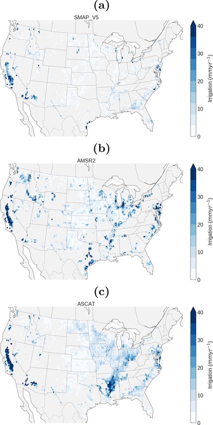
898                                  F. Zaussinger et al.: Estimating irrigation water use over the contiguous United States

   On the other hand, irrigation itself is an important anthro-     during a climatically dry and wet year on land–atmosphere
pogenic climate forcing (Sacks et al., 2009). It influences         interactions. They used the National Aeronautics and Space
the surface water and energy balance through directly in-           Administration’s (NASA) high-resolution Land Information
creasing soil moisture (SM). In turn, soil moisture is widely       System (LIS) and the NASA Unified Weather Research and
known to modulate the partitioning of energy between sensi-         Forecasting Model framework both in offline and coupled
ble and latent heat (Seneviratne et al., 2010). Subsequently,       simulations. In accordance with previous studies, they found
irrigation cools the land surface on local to regional scales       that irrigation indeed cools and moistens the surface over and
through increasing evapotranspiration (ET), whereas the in-         downwind of irrigated areas. Moreover, they found that the
creased availability of atmospheric water vapor can enhance         magnitude of this irrigation cooling effect strongly depends
cloud cover and precipitation (Boucher et al., 2004; Lobell         on the parametrization of the respective irrigation methods.
et al., 2006; Sacks et al., 2009). Researchers agree that irri-     In a very recent study, Kumar et al. (2018) conducted a multi-
gation may have masked the full warming signal caused by            sensor, multivariate land data assimilation experiment over
greenhouse gas emissions (Bonfils and Lobell, 2007; Kuep-           the CONUS by using the NASA LIS to enable the National
pers et al., 2007). As a past expansion of irrigated area and       Climate Assessment Land Data Assimilation System. Partic-
an overall increase in irrigation intensity may have signifi-       ularly, the use of a larger-than-normal range of soil moisture
cantly affected surface temperature observations, it is crucial     data records and snow depth data from microwave remote
to include irrigation impacts both in understanding histori-        sensing combined with an irrigation intensity map systemat-
cal climate and modeling future climate trends (Lobell et al.,      ically improved soil moisture and snow depth simulations.
2006). Assuming a similar expansion of irrigation as in re-            With respect to the discrepancies in the global modeling
cent decades, some regions may actually benefit from this ir-       studies, Sacks et al. (2009) argued that they can be primar-
rigation cooling effect. As outlined in Ozdogan et al. (2006),      ily explained by systematic differences in the control of irri-
ET and in turn irrigation water requirements can decrease           gation water application within the respective modules, e.g.,
within agricultural microclimates. However, nonlinear reper-        by climate, food demand and economical conditions. Logi-
cussions on temperature extremes can be expected when the           cally, this arguments also holds true for the modeling study
required water supply cannot be met (Thiery et al., 2017) and       by Lawston et al. (2015). Regarding the irrigation forcing
(semi-)arid regions are generally expected to be adversely af-      used in Kumar et al. (2018), we argue that the term “irrigation
fected by water scarcity (Kueppers et al., 2007). As a conse-       intensity” gives a false impression. Irrigation intensity in a
quence, especially in water-scarce regions, government agen-        physical sense should not be attributed to fractional irrigated
cies and water managers are challenged to increase water use        area but must rather be connected to the actual irrigation wa-
efficiency, optimize the distribution of water among farms          ter use (IWU) per unit area. In addition, fields may be either
and detect illegal groundwater pumping activities (Siebert          over- or under-irrigated with respect to the physically “ideal”
et al., 2010; Taylor et al., 2012). For example, as a conse-        amount. Hence, current irrigation modules are unable to con-
quence of prolonged winter precipitation deficits and positive      sistently reflect real-world conditions and thus introduce un-
temperature anomalies from 2012 to 2017, a record-breaking          certainties in modeling and data assimilation. Consequently,
drought peaking in 2015 affected the California Central Val-        information on the spatiotemporal distribution and develop-
ley. While farmers tried to compensate for the 2015 surface         ment of actual IWU is needed to improve the representation
water shortage by pumping more groundwater, a net water             of land–atmosphere feedbacks in model simulations (Ozdo-
shortage of over 3 km3 resulted in the fallowing of approxi-        gan et al., 2010a).
mately 230 000 ha of land (Howitt, 2015).
   To date, irrigation practices are typically not explicitly in-   1.1   Statistics on irrigated areas and water withdrawals
cluded in land surface, climate or weather models. On the
other hand, irrigation directly impacts land surface temper-        Available information on irrigated areas, and particularly ir-
ature, humidity and soil moisture observations, and through         rigation water use, lacks objectivity, spatial consistency and
them irrigation indirectly impacts model simulations when           temporal resolution needed for large-scale hydrological as-
they are being assimilated (Tuinenburg and Vries, 2017).            sessments and modeling (Deines et al., 2017). On local to
A range of climate modeling studies employed irrigation             regional scales, some irrigation districts conduct regular sur-
modules on a global scale. Mainly based on a combina-               veys, but often the data are not publicly available, lack geo-
tion of static spatial maps of irrigated area and soil mois-        referencing and are difficult to compare between regions due
ture and/or vegetation data, they tried to approximate sea-         to different sampling techniques. The elementary sources of
sonal IWU (Lobell et al., 2006; Bonfils and Lobell, 2007;           large-scale irrigation data are national and subnational statis-
Kueppers et al., 2007). However, the simulated impact of            tical units, which in most countries routinely collect infor-
irrigation on both global and regional climate showed con-          mation on irrigated area and/or irrigation water withdrawals
siderable variation across studies. With respect to a contigu-      (IWW). Data are usually represented as area equipped for
ous US (CONUS) domain, Lawston et al. (2015) assessed               irrigation (AEI) and in some cases also reflect the area ac-
the effects of drip, flood and sprinkler irrigation methods         tually irrigated (AAI) in the respective year of the census

Hydrol. Earth Syst. Sci., 23, 897–923, 2019                                        www.hydrol-earth-syst-sci.net/23/897/2019/
F. Zaussinger et al.: Estimating irrigation water use over the contiguous United States                                       899

(Siebert et al., 2005). The Global Map of Irrigation Areas         on local, regional and global scales. Vegetation indices have
(GMIA) was the first global-scale geospatial irrigated area        been identified as effective proxies for irrigation practices,
data set (Döll, 2002; Döll and Siebert, 2002) based on such        because irrigated and non-irrigated croplands show differ-
statistics. GMIA combines subnational irrigation data from         ent spectral responses during the peak growing season (Oz-
various sources (FAO, UN, World Bank, agriculture depart-          dogan et al., 2010b). A wide range of studies used vegeta-
ments) and geospatial information on the location and extent       tion indices to map annual irrigated areas and their changes
of irrigation schemes (point, polygon and raster data, land        through time, sometimes in combination with statistical in-
cover maps and satellite imagery) to map AEIs and AAIs at          ventory data.
0.5◦ resolution around the year 2000. In subsequent versions          Only few global land-use–land-cover (LULC) maps based
the resolution was improved to 5 armin ×5 arcmin (Siebert          on optical remote sensing separate irrigated from rain-fed
et al., 2005, 2007) and a new global historical irrigation data    croplands. For example, the United States Geological Survey
set providing time series of AEI between 1900 and 2005 was         (USGS) Global Land Cover Characteristics (GLCC) data set
developed (Siebert et al., 2015). However, the large variabil-     was derived from 1 km Advanced Very High Resolution Ra-
ity in the quality of the underlying statistical inventory data    diometer (AVHRR) sensor data and identified four types of
is propagated into the uncertainty of the final spatial map        irrigated croplands in the year 1992 (Loveland et al., 2000).
(Siebert et al., 2005).                                            However, the classification algorithms used were not tai-
   In summary, the main limitations of statistical inventories     lored to irrigated area mapping, thus resulting in low clas-
and derived products are the following.                            sification accuracies. Large discrepancies were found be-
                                                                   tween USGS GLCC and country-level reports of irrigated
 1. The quality of the data varies significantly among coun-
                                                                   area, originating from both the uncertainties of the inven-
    tries (Siebert et al., 2010). While for instance the United
                                                                   tory data and technical limitations of the remote sensing data
    States agricultural census is considered to have high
                                                                   sets (Vörösmarty et al., 2000). Through a combination of un-
    quality, many developing countries lack the resources
                                                                   supervised clustering and expert knowledge, the European
    for comprehensive reporting.
                                                                   Space Agency (ESA) Climate Change Initiative (CCI) has
 2. National statistics are usually only valid for single years    produced a global land cover product at 300 m resolution
    and depend on the individual compilation cycle of each         using Medium Resolution Imaging Spectrometer (MERIS)
    country (e.g., every 5 years in the case of the US).           data (Bontemps et al., 2013). It distinguishes between irri-
                                                                   gated and non-irrigated croplands for 2000, 2005 and 2010.
 3. Irrigated area estimates usually reflect areas equipped
                                                                   However, we argue that over the CONUS the irrigated class is
    for irrigation, rather than areas actually irrigated. De-
                                                                   likely to be considered unreliable, as apparently all irrigated
    pending on climatic and market conditions, farmers may
                                                                   lands are wrongly attributed to the non-irrigated agriculture
    decide to only cultivate and irrigate a portion of their
                                                                   class.
    fields.
                                                                      Other studies used approaches specifically tailored to ir-
 4. Irrigation volume estimates reflect irrigation water with-     rigated area mapping. For instance, the global data set of
    drawals rather than actual irrigation water use (e.g., if      monthly irrigated and rain-fed crop areas around the year
    rainfall is sufficient, already withdrawn spare water is       2000 (MIRCA2000) provides irrigated and rain-fed areas
    stored in reservoirs instead of being irrigated).              for 26 crop classes for each month of the year at 5 arcmin
                                                                   resolution (Portmann et al., 2010). For this purpose, agri-
 5. Naturally, survey-based statistics are only based on a         cultural census statistics, national reports, databases, a map
    sample of farms, which may not be representative.              of crop-specific annual harvested area, a cropland extent
 6. Conventional methods are unable to reflect illegally           map, the GMIA, crop calendars, and ancillary information
    withdrawn water used for irrigation (Roseta-Palma              on climate and topography were combined. Using quantita-
    et al., 2014; Saffi and Cheddadi, 2010).                       tive spectral matching techniques on normalized difference
                                                                   vegetation index (NDVI) time series from multiple sensors
   On the basis of these drawbacks, remote sensing evolved
                                                                   (AVHRR, SPOT-1, MODIS, Landsat 7 and JERS-1 SAR) in
as an effective tool to potentially overcome these limitations
                                                                   combination with climate (monthly precipitation and temper-
since it provides synoptic, independent and timely informa-
                                                                   ature data from the Climate Research Unit) and ancillary data
tion of biogeophysical variables that are either directly or in-
                                                                   (GTOPO30 1 km digital elevation model, global tree cover),
directly related to irrigation.
                                                                   the International Water Management Institute (IMWI) pro-
1.2     Remote sensing for irrigation mapping                      duced a Global Irrigated Area Map (GIAM) at 1 km resolu-
                                                                   tion around the year 2000 (Thenkabail et al., 2009). More re-
1.2.1    Optical and thermal remote sensing                        cently, Salmon et al. (2015) created a global map of rain-fed,
                                                                   irrigated and paddy croplands (GRIPC) around the year 2005
Data acquired by optical sensors (AVHRR, MODIS, Land-              at 500 m spatial resolution using supervised classification
sat) have been extensively used to identify irrigated areas        of remote sensing, climate and agricultural inventory data.

www.hydrol-earth-syst-sci.net/23/897/2019/                                        Hydrol. Earth Syst. Sci., 23, 897–923, 2019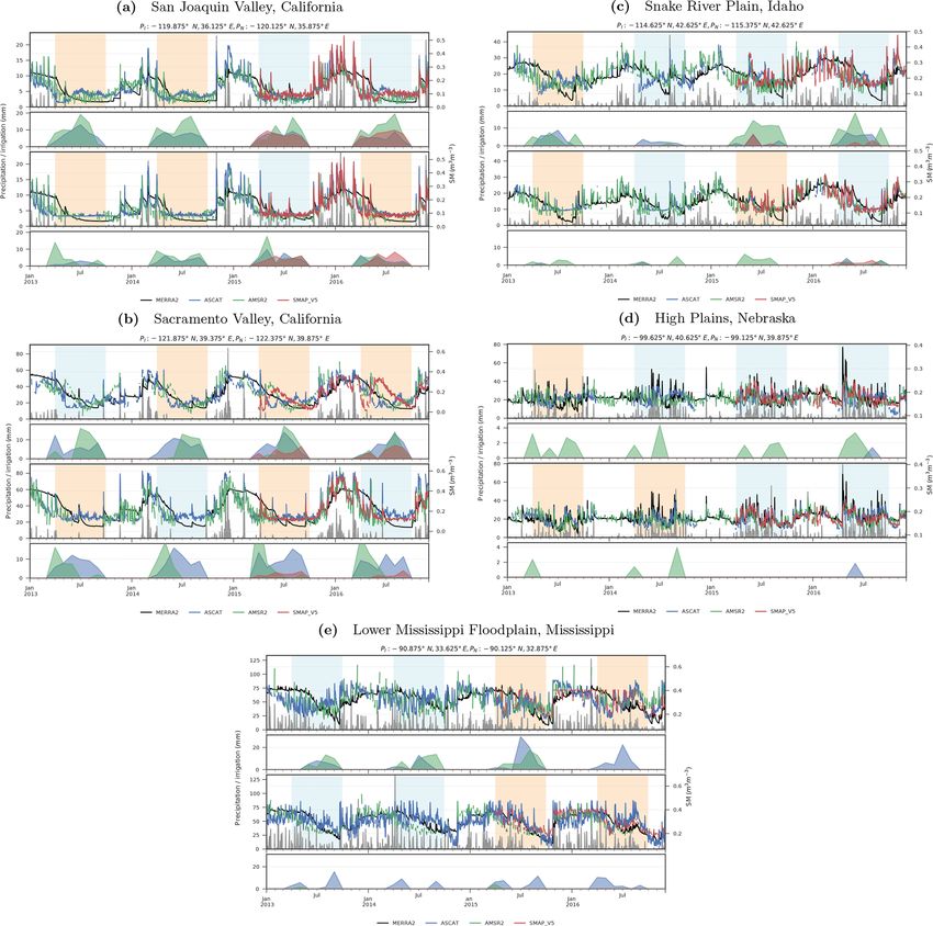
900                                  F. Zaussinger et al.: Estimating irrigation water use over the contiguous United States

However, there are large discrepancies between the different        heat flux (LE). They compared modeled bottom-up LE (i.e.,
global data sets mainly stemming from varying definitions           without irrigation) and top-down LE drawn from observa-
of irrigated areas among the data sets (i.e., area equipped for     tions of diurnal land surface temperature changes which are
irrigation, irrigated area and cropped area) and differing ref-     connected to changes in the land surface moisture status and
erence years (i.e., the years 2000 and 2005) (Salmon et al.,        therefore irrigation. However, these methods are only able to
2015; Meier et al., 2018). Moreover, three of the four ex-          provide estimates on irrigation water requirements (i.e., what
isting global maps (GMIA, MIRCA2000 and GRIPC) rely                 amount of water a plant would ideally need), as opposed to
on agricultural inventory data for the classification of irri-      actually irrigated water, as in practice fields are often under-
gated areas, which is subject to major limitations concerning       irrigated.
quality and accuracy. In addition, the maps are limited to sin-
gle years (GMIA, GIAM, GRIPC) or single months within               1.2.2   Microwave remote sensing
a single year (MIRCA2000), thus not being able to address
the high inter-annual variability of irrigated areas, which is      Microwave observations are widely used to estimate soil
mainly governed by climate and market conditions (Deines            moisture (Entekhabi et al., 2010; Wagner et al., 2013; Dorigo
et al., 2017).                                                      et al., 2017). The major advantages of microwave observa-
   On a continental scale, the MODIS Irrigated Agriculture          tions are their all-weather capability and the intrinsic capac-
Dataset for the conterminous United States (MIrAD-US) was           ity to sense a geophysical variable which is directly and phys-
created by assimilating county-level irrigation statistics with     ically linked to irrigation.
MODIS-derived seasonal peak NDVI to spatially identify ir-             The first study to investigate the utility of satellite soil
rigated and non-irrigated lands at 250 m resolution (Ozdogan        moisture retrievals for irrigation mapping was carried out by
and Gutman, 2008; Pervez et al., 2008; Pervez and Brown,            Kumar et al. (2015). They used soil moisture retrievals from
2010). A significant drawback is that the map compilation is        ASCAT, AMSR-E, SMOS and WindSat, and the ESA CCI
tied to the same 5-year cycle of the United States Department       multi-satellite surface soil moisture product in combination
of Agriculture (USDA) Census of Agriculture. Ambika et al.          with soil moisture estimates from the Noah LSM (land sur-
(2016) mapped irrigated areas from 2000 to 2015 at 250 m            face model) to map irrigated areas in the CONUS. Their key
resolution over India by using 250 m MODIS seasonal peak            assumption was that irrigation is not included in the formu-
NDVI data and 56 m LULC data. Teluguntla et al. (2017)              lation of LSM, whereas satellite-derived soil moisture is ex-
used spectral matching techniques and automated cropland            pected to reflect the changes in soil moisture induced by irri-
classification algorithms to infer cropland extent, irrigated       gation. Based on synthetic data, they were able to detect dif-
versus rain-fed croplands, and cropping intensities over Aus-       ferences between the probability density functions of satel-
tralia. The latter two products allow for the study of inter-       lite and modeled soil moisture. However, the satellite data
annual variability of irrigated areas (Ambika et al., 2016).        showed only few systematic differences that could be reli-
   On a regional scale, higher-resolution Landsat imagery           ably related to irrigation practices.
was adopted by a range of studies. Ozdogan et al. (2006)               Qiu et al. (2016) compared trends from 1996 to 2010 in
used 30 m Landsat imagery to map changes in annual irri-            China of ESA CCI, ERA-Interim/Land reanalysis and in
gated area from 1993 to 2002 in southeastern Turkey based           situ soil moisture, as well as precipitation. They observed
on NDVI thresholding approaches and compared them with              significant discrepancies between precipitation and satellite
estimates of irrigation water requirements inferred from po-        soil moisture trends over irrigated areas, which they ascribed
tential evapotranspiration. In a recent study, Deines et al.        to irrigation. Escorihuela and Quintana-Seguí (2016) com-
(2017) produced annual irrigation maps for 1999–2016 for            pared three global satellite soil moisture products (ASCAT,
a region in the High Plains aquifer (United States) at 30 m         AMSR2 and SMOS) with model soil moisture estimates
resolution. Pun et al. (2017) used a combination of surface         from the Surface Externalisée (SURFEX) model (Masson
energy balance partitioning and vegetation indices to clas-         et al., 2013) (forced with meteorological data) in the Mediter-
sify irrigated and non-irrigated croplands at 30 m resolution       ranean. Only a downscaled version of SMOS (SMOScat)
in Nebraska.                                                        showed significantly lower correlations over irrigated areas.
   Thermal remote sensing has been widely used to map irri-         The authors argued that primarily due to the coarse spa-
gation water based on estimating potential evaporation from         tial resolution of the native soil moisture retrievals the other
surface energy heat fluxes and the application of specific          products were not able to resolve the irrigation signal from
crop factors (Rosas et al., 2017). A well-known technique           the soil moisture signal from the surrounding dry-land area.
is the Surface Energy Balance Algorithm for Land, which             Very recently Lawston et al. (2017) investigated the potential
estimates variables of the hydrological cycle based on re-          of the new SMAP (Soil Moisture Active Passive mission)
motely sensed surface energy balance components (Basti-             enhanced 9 km SM product to identify irrigation signals in
aanssen et al., 1998). In contrast, Hain et al. (2015) developed    three semi-arid regions in the western United States. Results
a novel method for inferring regions where non-precipitation        showed that SMAP soil moisture carries a clear irrigation sig-
inputs (e.g., irrigation) significantly impact terrestrial latent   nal from rice irrigation in the Sacramento Valley (California),

Hydrol. Earth Syst. Sci., 23, 897–923, 2019                                        www.hydrol-earth-syst-sci.net/23/897/2019/
F. Zaussinger et al.: Estimating irrigation water use over the contiguous United States 901
while the signals were less obvious in the other two regions
(Columbia River basin, Washington and Colorado).
1.3 Objective of this study
Despite the large number of studies using remote sensing ap-
proaches to map irrigated area and irrigation water require-
ments at various spatial and temporal scales, none of these
approaches has attempted to derive actual irrigation water
use. To bridge this gap, we propose a new method for es-
timating IWU from a combination of remotely sensed and
modeled reanalysis soil moisture data. The approach is based
on the hypothesis that neither the structure nor the forc-
ing of the model data accounts for artificial water supply,
while the microwave soil moisture retrievals do (Kumar et al.,
2015; Escorihuela and Quintana-Seguí, 2016). The method
is implemented over the CONUS by using three state-of-the-
art microwave soil moisture products (i.e., based on SMAP,
AMSR2 and ASCAT) in combination with MERRA-2 re-
analysis soil moisture. By using passive L-band and both
active and passive C-band soil moisture data, we aim to as-
sess the impact of the microwave observation frequency and
the sensing technique with respect to irrigation quantifica-
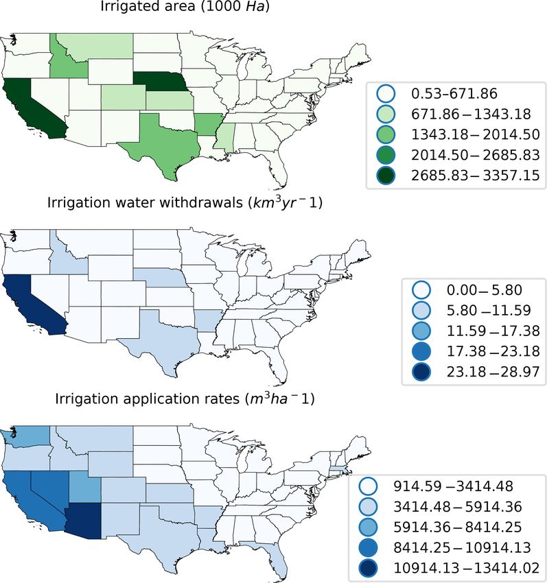
tion. For this reason we only used one data set per category. Figure 1. Per-state irrigated area, irrigation water withdrawals and
The paper is organized as follows: Sect. 2 provides a gen- irrigation water application rates for 2013. The data were drawn
eral overview of the irrigation landscape in the CONUS. from the latest Farm and Ranch Irrigation Survey (FRIS) and only
reflect irrigation operations in open fields (e.g., excluding crops
Section 3 covers the utilized satellite, model and ancillary
grown and irrigated in greenhouses).
data sets and the preprocessing involved. The theoretical
and practical aspects of the new methodology to estimate
IWU are discussed in Sect. 4. Results are shown and dis- specific crop type, water source and irrigation technique. In
cussed with respect to official reference irrigation data in addition, these estimates are given for crops cultivated out-
Sect. 5. Section 6 concludes the study and gives an outlook doors (“in the open”) and indoors (“under protection”, e.g.,
on follow-on research. horticultural crops grown in greenhouses). Figure 1 shows
the per-state irrigated area and irrigation water withdrawals
2 Study area limited to crops grown outdoors, as well as irrigation applica-
tion rates during the 2013 growing season provided by FRIS.
2.1 Irrigation practices in the contiguous United States It is likely that the sensitivity of satellite soil moisture re-
trievals to irrigation increases when the irrigation application
The amount of water needed by a certain crop for optimal efficiency of a particular irrigation system or technique de-
growth mainly depends on three factors: crop type, soil and teriorates. Therefore, we expect higher sensitivity towards
climate. Irrigation water need is given by the difference be- gravity irrigation systems (e.g., flood and furrow irrigation)
tween these requirements for optimal crop growth and effec- and lower sensitivities towards sprinkler and micro-irrigation
tive rainfall. In the largely semi-humid climate of the eastern systems. Figure A1 shows a distinct decline in irrigation rates
United States, irrigation is supplemental, which means that per area from the semi-arid west to the more humid east. The
irrigation is applied to mostly rain-fed crops during times of state of Arizona has the highest irrigation rate per area, fol-
insufficient rainfall to achieve higher yields than under rain- lowed by California and Nevada. Gravity flow systems show
fed conditions alone. In contrast, the predominantly semi- the highest rates in California and Arizona but also depict
arid climate of the western US makes artificial water supply large values along the Mississippi Delta. This can mainly
a necessity, thus requiring full irrigation. be attributed to the cultivation of rice, which is primarily
The 2013 Farm and Ranch Irrigation Survey (FRIS) of grown in these regions and is either flood or furrow irrigated.
the National Agricultural Statistics Service (NASS) of the Finally, micro-irrigation systems are largely limited to the
USDA provides selected irrigation data from surveys con- western half of the US.
ducted at approximately 35 000 farms using irrigation across
the US (USDA, 2013). It reports state-level data of both ir-
rigated area and irrigation water withdrawals subdivided by
www.hydrol-earth-syst-sci.net/23/897/2019/ Hydrol. Earth Syst. Sci., 23, 897–923, 2019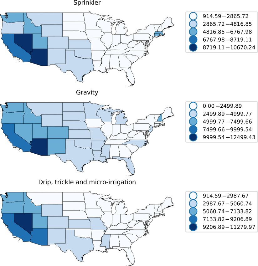
902                                   F. Zaussinger et al.: Estimating irrigation water use over the contiguous United States

                                                                      ally supplied by winter snowmelt. In the Sacramento Val-
                                                                      ley, which accounts for 95 % of California’s rice yield, rice
                                                                      is typically water seeded (Linquist et al., 2015). This means
                                                                      that the fields are completely flooded at 10–15 cm depth be-
                                                                      fore planting (usually late April to mid-May) and then seeded
                                                                      with the help of airplanes. The fields typically remain flooded
                                                                      throughout the growing season and are only drained from
                                                                      early September onward, approximately 3 weeks before har-
                                                                      vest in September to mid-October.

                                                                      2.2.2   Snake River Plain, Idaho

                                                                      Idaho accounts for the second largest irrigation water with-
Figure 2. Study regions and locations of the pixels selected for      drawals in the US after California (NASS, 2012). In Idaho,
a local time series analysis over the fractional irrigated area map   the Snake River Plain is the most important agricultural area
derived from the spatially aggregated MIrAD-US data set (Per-
                                                                      and sprinkler irrigation is the dominant irrigation technique.
vez and Brown, 2010). The focus regions are included in black
squares and include the Sacramento Valley (SV) and San Joaquin
                                                                      Similar to the San Joaquin Valley it is characterized by a cold
Valley (SJV) in the California Central Valley (CCV), Snake River      semi-arid climate (Kottek et al., 2006).
Plain (SRP), Nebraska Plains (NPS) and the Mississippi Floodplain
(MFP). Green and orange crosses indicate the locations of the ir-     2.2.3   High Plains, Nebraska
rigated (PI) and non-irrigated (PNI) pixels, respectively, at which
we further analyze satellite and model soil moisture time series in   Nebraska is located in the middle of a transitional climate
conjunction with IWU estimates.                                       zone which extends longitudinally through the middle of the
                                                                      US. While the climate in western Nebraska is cold semi-arid,
                                                                      the eastern part is humid continental, characterized by hot
2.2     Focus areas                                                   summers and year-round precipitation (Kottek et al., 2006).
                                                                      For example, irrigation requirements for corn are approxi-
In addition to the continental-scale analysis, we chose four          mately 350 mm in the west and continuously drop to ap-
irrigation hot spots characterized by different climates and          proximately 150 mm in the east (reference values obtained
irrigation practices within the CONUS (Fig. 2) to compre-             from the University of Nebraska–Lincoln). The mainly em-
hensively assess the spatiotemporal dynamics of irrigation.           ployed irrigation system is the center pivot, and the major
These regions are the Sacramento Valley and San Joaquin               crops grown are corn and soybean.
Valley in the California Central Valley; the Snake River
Plain, Idaho; the High Plains, Nebraska; and part of the Mis-         2.2.4   Mississippi Floodplain, Mississippi
sissippi Floodplain located within the state of Mississippi.
For each focus area, we conducted a time series analysis at a         The Mississippi Floodplain region is characterized by a fully
local scale (Sect. 5.3), as well as a cross comparison with ref-      humid subtropical climate with hot summers (Kottek et al.,
erence data on irrigated area (Sect. 5.5) and irrigation water        2006). Despite the large amounts of rainfall throughout the
withdrawals (Sect. 5.4).                                              year, only approximately 30 % falls in the summer period
                                                                      when the major crops are grown (Kebede et al., 2014), thus
2.2.1    Central Valley, California                                   requiring the use of supplemental irrigation. The dominant
                                                                      crop types include soybean, corn, cotton and rice. Within the
Traditionally, the California Central Valley accounts for the         Mississippi Floodplain we chose an area in the state of Mis-
highest irrigation water withdrawals across the CONUS. Its            sissippi for a local analysis. Here, reports on irrigation water
northern part is characterized by a Mediterranean climate             withdrawals (2009 and 2011 growing seasons) are available
with hot, dry summers, whereas its southern half is defined           from the Yazoo Mississippi Delta Joint Water Management
by both hot and cold semi-arid climates (Kottek et al., 2006).        District. For the 2011 growing season, average application
As a result, crop production requires full irrigation. We se-         rates of approximately 180, 400, 330 and 970 mm are re-
lected two areas within the Central Valley for the time series        ported for cotton, corn, soybeans and rice, respectively, lead-
analysis: the southern San Joaquin Valley, where several dif-         ing to an average of around 490 mm.
ferent crop types are cultivated using sprinkler, furrow and
micro-irrigation systems, and the northern Sacramento Val-
ley, where flood irrigation for rice is prevalent and which was
also investigated by Lawston et al. (2017). Rice production
in California is the second largest in the US (NASS, 2012)
and relies on large amounts of irrigation water, which is usu-

Hydrol. Earth Syst. Sci., 23, 897–923, 2019                                          www.hydrol-earth-syst-sci.net/23/897/2019/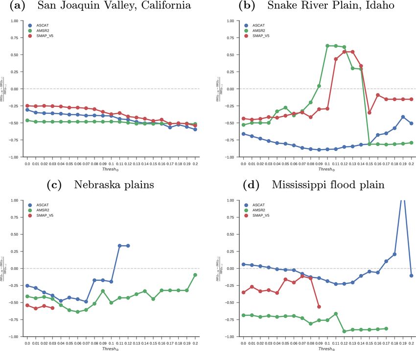
F. Zaussinger et al.: Estimating irrigation water use over the contiguous United States 903
3 Data sources
The data sources used in this study are summarized in Ta-
ble 1.
3.1 Remotely sensed soil moisture
3.1.1 SMAP
mm day−1
cm3 cm−3
m3 m−3
m3 m−3 The Soil Moisture Active Passive (SMAP) mission was
Units
launched in January 2015 and is the second mission exclu-
%
–
–
sively designed for the retrieval of soil moisture together with
freeze and/or thaw status (Entekhabi et al., 2010). After fail-
Native gridding
0.625◦ × 0.5◦
ure of its radar in July 2015, the radiometer continues to
provide measurements in the L band (1.4 GHz) at a spatial
12.5 km
36 km
300 m
250 m
resolution of approximately 40 km. Validation studies have
0.25◦
0.25◦
shown that the radiometer meets the target retrieval accuracy
of 0.04 m3 m−3 (unbiased RMSE, ubRMSE) over non-frozen
land surfaces free of excessive snow, ice, mountainous ter-
0.25◦ (resampled)
0.25◦ (resampled)
Spatial resolution
rain and dense vegetation coverage (Colliander et al., 2017).
In general, the L band is expected to be more suitable for
∼ 40 km
∼ 40 km
∼ 25 km
∼ 50 km
soil moisture retrieval, because it is less affected by vege-
0.25◦
tation and representative of a deeper soil layer than higher
frequency C- or X-band retrievals (Entekhabi et al., 2010).
SMAP obtains global coverage every 2–3 days and equa-
Temporal resolution
torial crossing times are 06:00 and 18:00 local solar time
1 day (resampled)
(LST) for the descending and ascending orbits, respectively.
We used both ascending and descending orbit data covering
∼ 1.5 days
1–3 days
1–2 days
the period of April 2015 to December 2016. We used the
L3_SM_P V5 data product, which is sampled at 36 km res-
1 day
olution. In this product version, a water body correction and
–
–
an improved soil temperature depth correction have been ap-
01/2007–12/2016
plied, which have respectively reduced anomalous soil mois-
04/2015–present
07/2012–present
01/2007–present
01/1980–present
Data availability
reference time
ture values near large water bodies and the dry bias with re-
2008–2012
spect to the SMAP core validation sites (Jackson, 2018). In
the case of overlapping orbits, we only used the descending
2012
(06:00 LST) overpass.
3.1.2 AMSR2
M2T1NXLND.5.12.4 (SFMC
Unified Gauge-Based Analysis
MODIS Irrigated Agriculture
Dataset for the United States v3
AMSR2 is a microwave radiometer on board the GCOM-W1
satellite and has provided measurements at 6.9 GHz (C band)
of Daily Precipitation
LC map 2010 epoch
and three higher frequencies up to 36.5 GHz (Ka band) since
July 2012 (Imaoka et al., 2010). Daily ascending and de-
modified H111
SMAP_L3_v4
Product name
scending overpasses are at 13:30 and 01:30 LST, respec-
LPRM v06
parameter)
tively, achieving global coverage with a spatial resolution of
about 40 km every 1–2 days. The VUA–NASA product used
in this study is based on the Land Parameter Retrieval Model
(LPRM) V6 algorithm, which simultaneously retrieves vol-
ESA CCI Land Cover
Table 1. Data products.
umetric soil moisture and vegetation optical depth (VOD)
from the observed brightness temperatures (Owe et al., 2008;
CPC precipitation
der Schalie et al., 2016). LPRM is based on a radiative trans-
fer equation and partitions the observation into its emission
MIrAD-US
MERRA-2
components from soil and vegetation based on the horizontal
AMSR2
ASCAT
SMAP
and vertical polarized brightness temperatures. Only obser-
Data
vations from the descending orbits were used and, in addi-
www.hydrol-earth-syst-sci.net/23/897/2019/ Hydrol. Earth Syst. Sci., 23, 897–923, 2019
904                                 F. Zaussinger et al.: Estimating irrigation water use over the contiguous United States

tion, the retrievals were masked for high VOD values and          tions (Reichle et al., 2017c), which are directly impacted by
radio frequency interference (RFI), spatially resampled to        irrigation (Wei et al., 2013; Tuinenburg and Vries, 2017).
a regular 0.25◦ grid and temporally centered at 00:00 UTC         MERRA-2 surface soil moisture simulations were evaluated
(Dorigo et al., 2017; Gruber et al., 2017; Liu et al., 2012).     in Reichle et al. (2017b) with in situ soil moisture data from
                                                                  320 sites. It was shown that the modeled estimates are biased
3.1.3    ASCAT                                                    by 0.053 m3 m−3 , which is approximately in the order of the
                                                                  SMAP soil moisture retrieval target accuracy.
The Advanced Scatterometer (ASCAT) on board the Mete-
orological Operational (Metop-A and B) satellites has been        3.3   Ancillary data
operational since October 2006 and is a real aperture radar
instrument operating at C band (5.255 GHz) and VV polar-          Despite the drawbacks discussed in Sect. 1.2, the ESA CCI
ization. Local equatorial crossing times are at 21:30 for the     Land Cover data set (Bontemps et al., 2013) was used to cre-
ascending overpass and at 09:30 for the descending overpass,      ate a cropland mask for the CONUS, because the classifi-
and global coverage is achieved every 1–3 days depending on       cation of overall agricultural land cover (i.e., irrigated and
latitude. The TU Wien change detection algorithm (Wagner          rain-fed lands) proved to be accurate. For a more detailed
et al., 1999; Naeimi et al., 2009) is applied to the backscat-    analysis of the impact of precipitation, we used CPC Unified
ter coefficients to create time series of relative surface soil   Gauge-Based Analysis of Daily Precipitation, which covers
moisture for the topmost centimeters of soil. This is accom-      the CONUS at 0.25◦ native resolution (Chen et al., 2008;
plished by scaling each observation between reference val-        Xie et al., 2010). Therefore, it is expected to provide more
ues representing the historically lowest and highest observed     detailed information than the precipitation data set used to
backscatter values, respectively. Soil moisture is provided       force MERRA-2 SM, which has a 0.5◦ resolution.
in degree of saturation (%) and ranges between 0 % (wilt-
ing point) and 100 % (soil saturation). It has a spatial reso-    3.4   Data preprocessing
lution of 25 km and is made available on a discrete global
grid (DGG) at a spatial sampling of 12.5 km. In this study,       As data from SMAP were only available from April 2015
we used a modified version of the European Organisation           onward, we extended the study period to include available
for the Exploitation of Meteorological Satellites (EUMET-         AMSR2 and ASCAT data from 2013 to 2016. Hence, four
SAT) Satellite Application Facility on Support to Operational     growing seasons with varying climatic conditions were cov-
Hydrology and Water (H-SAF) H111 soil moisture product.           ered by the AMSR2 and ASCAT sensors and two growing
The modified version uses a dynamic correction which is ex-       seasons by SMAP. We assumed a general growing season
pected to better account for inter-annual variability than the    for the entire CONUS from the start of April to the end of
original H111 product (Hahn et al., 2017; Vreugdenhil et al.,     September. All data were spatially matched to a common
2016).                                                            0.25◦ regular grid using nearest-neighbor resampling. In or-
                                                                  der to constrain the analysis to areas where irrigation is fea-
3.2     MERRA-2 reanalysis soil moisture                          sible, we masked all pixels with < 5 % of fractional crop-
                                                                  land area based on ESA CCI Land Cover for 2010 (Bon-
The second Modern-Era Retrospective analysis for Research         temps et al., 2013). Unreliable observations in the satellite
and Applications 2 (MERRA-2) (Bosilovich et al., 2016) is         data were masked, applying their respective quality flags for
an atmospheric reanalysis product providing global, hourly        frozen soil, dense vegetation and radio frequency interfer-
fields of land surface and atmospheric conditions for 1980–       ence.
present at a spatial resolution of 0.625◦ × 0.5◦ . It assimi-        The spatial representativeness and observation depth
lates atmospheric satellite observations using the Goddard        slightly differ among the various remote sensing products
Earth Observing System Model (GEOS-5). MERRA-2 uses               and modeled soil moisture. MERRA-2 SM is simulated for
an observation-based precipitation correction over land to        a fixed 5 cm thick soil layer (Bosilovich et al., 2016) and
fully correct modeled precipitation at latitudes < |42.5◦ |,      thus shows more inertia to changes in the water balance
with a linear tapering between |42.5◦ | < latitude < |62.5◦ |,    (i.e., through precipitation) than the remotely sensing data.
while no correction is applied at more northern and south-        Besides, ASCAT is provided in a different unit than the
ern latitudes. The precipitation correction has significantly     other products. To account for these systematic differences
improved the soil moisture simulations with respect to its        between products, we applied a linear rescaling approach
predecessor (Reichle et al., 2017a). The soil moisture sim-       (Brocca et al., 2013), which forces the satellite soil mois-
ulations are representative of the first 5 cm of soil and are     ture time series 2sat to have the same mean µ and standard
expressed in volumetric units (m3 m−3 ). We explicitly chose      deviation σ as the modeled soil moisture 2mod :
MERRA-2 soil moisture in favor of soil moisture from other
global reanalysis data sets, because MERRA-2 does not as-                       2sat − µ(2sat )
similate surface humidity and surface temperature observa-        2sat
                                                                   rescaled =                   σ (2mod ) + µ(2mod ).        (1)
                                                                                   σ (2sat )

Hydrol. Earth Syst. Sci., 23, 897–923, 2019                                       www.hydrol-earth-syst-sci.net/23/897/2019/
F. Zaussinger et al.: Estimating irrigation water use over the contiguous United States                                        905

It is likely that over irrigated areas µ(2sat ) increases during   Hence, estimating irrigation from differences between the
the respective irrigation period, which alters the scaling pa-     temporal variations of satellite and model SM is theoretically
rameters. We expect that this should not affect the temporal       feasible.
evolution of changes in soil moisture. However, the influence
of irrigation on the temporal variability of soil moisture (de-    4.2   Deriving irrigation water use
pending on the type of irrigation, general climate conditions,
etc.) is a source of uncertainty. In particular over very dry      We define an irrigation event   as a simultaneous increase in
                                                                                               sat
regions, the model soil moisture may never reach saturation,       satellite soil moisture d2dt > 0 and a decrease or stagna-
while the remotely sensed soil moisture data do (due to ir-
                                                                                                    mod
                                                                   tion in model soil moisture d2dt ≤ 0 . This means that
rigation). Since the variable of interest is irrigation amount,
volumetric soil moisture in m3 m−3 is converted to the corre-      rainfall did not cause the satellite-observed increase in soil
sponding water column depth Dwatertable (mm) by multiply-          moisture, which over agricultural land was very likely a re-
ing it with the depth of soil Dsoil for which the soil moisture    sult of irrigation. For each event, the amount of irrigation
simulations are representative. Thus, for the layer 0–5 cm, for    water leading to the increase is derived as the difference
                                                                   d2sat    d2mod
example, 0.3 m3 m−3 corresponds to a 15 mm water column              dt − dt , if the change in satellite is significant (i.e.,
covering the unit area of 1 m2 .                                   above the noise level). The latter is accounted for by apply-
                                                                   ing a threshold of relative soil moisture change thresh2 (see
                                                                   Sect. 4.3 and Appendix A). We then calculate seasonal irri-
4     Methods                                                      gation water use (IWU) summing up the approximated dif-
                                                                   ference quotients over the growing season period:
4.1    Theoretical foundation for retrieving irrigation
                                                                           iZ
                                                                            EOS
       water use from microwave remote sensing                                                            EOS
                                                                                                          X
                                                                   IWU =          (d2sat   mod
                                                                                     i − d2i   ) dt ≈            12sat-mod
                                                                                                                   i       ,   (5)
Kumar et al. (2015) first proposed the idea of inferring ir-               iSOS
                                                                                                         i=SOS
rigation from a positive bias between remotely sensed and
modeled soil moisture, induced by seasonal water application       where
                                                                                       12sat    mod , if 12sat ≥ 2

during the dry season. This idea is based on two key assump-
                                                                   12sat-mod =            i − 12i           i     thresh
tions: first, the satellite soil moisture products are sensitive     i                 0,             otherwise
to large-scale irrigation (as partly confirmed by Escorihuela
                                                                   and with
and Quintana-Seguí, 2016; Lawston et al., 2017); and, sec-
ond, the model does not account for irrigation, neither ex-        12sat  sat  sat
                                                                     i = 2i − 2i−n ,
plicitly (i.e., in the formulation) nor implicitly through the     12mod = 2mod − 2mod
                                                                     i      i      i−n .
assimilation of surface humidity or surface temperature ob-
servations, which are affected by irrigation (Wei et al., 2013).   IWU is the accumulated irrigation water use from the start
We build on these assumptions and introduce a new metric to        (iSOS ) until the end of the growing season (iEOS ). According
estimate IWU from the difference between satellite-observed        to the crop calendars provided by Portmann et al. (2010) and
and modeled soil moisture. The soil water balance equations        the USDA planting and harvesting dates handbook (NASS,
describing the respective change in soil moisture for each         2010) the period 1 April–30 September generally covers the
time step t (day) are described by                                 growing season of most crops receiving irrigation water in
                                                                   the CONUS. 2sat   i and 2i
                                                                                               mod are satellite and model SM on
d2sat                                                              day i, thresh2 denotes the relative soil moisture threshold,
      = P (t) + I (t) − ET(t) − R(t) − 1Srest               (2)
 dt                                                                and 2sat           mod
                                                                           i−n and 2i−n are the last available soil moisture ob-
                                                                   servations with a data gap of n days. If an irrigation event is
for the satellite observations and
                                                                   detected during an observation gap of > 4 days, we check if
d2mod                                                              there has been a significant increase in the model soil mois-
      = P (t) − ET(t) − R(t) − 1Srest                       (3)    ture (e.g., due to rainfall) within that period. When more
  dt
                                                                   than one significantly positive model slope (or precipitation
for the model simulations. P (mm) is precipitation; I (mm) is      events) occurs during the gap period, we cannot say for sure
irrigation; ET (mm) is evapotranspiration; and 2sat and 2mod       if the observed increase in soil moisture was due to irriga-
(mm) are satellite and modeled surface soil moisture, respec-      tion or precipitation and therefore conservatively disregard
tively, converted to water column depth. 1Srest (m3 m−3 ) de-      the potential irrigation event.
scribes water storage changes below the surface layer, includ-
ing drainage. Subtracting Eq. (3) from Eq. (2) yields              4.3   Masking spurious irrigation detections

          d2sat d2mod                                              It is essential to differentiate between irrigation signals and
I (t) =        −      .                                     (4)    high-frequency noise in the satellite data. For this purpose,
           dt     dt

www.hydrol-earth-syst-sci.net/23/897/2019/                                             Hydrol. Earth Syst. Sci., 23, 897–923, 2019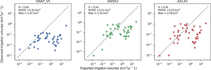
906 F. Zaussinger et al.: Estimating irrigation water use over the contiguous United States
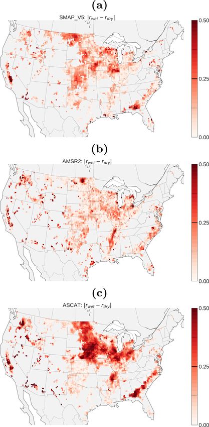
we apply a threshold thresh2 to the relative changes in satel- rigated (as inferred from the MIrAD-US product) while r wet
lite soil moisture similar to the approach applied by Dorigo is strongly positive, this is a strong indication of irrigation
et al. (2013) to detect spurious in situ data: (also see Fig. A2, where the absolute differences between
the mean correlations for wet and dry periods |rwet −rdry | are
2sat sat
t − 2t−n shown).
≥ 0.12 ≡ thresh2 . (6)
2sat
t−n Over non-agricultural land cover, low growing season cor-
relations between SMAP and MERRA-2 soil moisture are
Based on an extensive sensitivity analysis (Appendix A) we observed over the densely vegetated south- and northeastern
concluded that a threshold of thresh2 ≡ 0.12 is an appropri- US, as well as over parts of the arid southwest (Fig. 3a, b).
ate generic choice for the whole CONUS. AMSR2 exhibits low correlations in coastal areas, complex
Potential errors may arise when the model forcing misses terrain and over dense vegetation cover (Fig. 3c, d). ASCAT
or creates false rainfall events. In addition, because of dif- shows negative correlations against MERRA-2 over the arid
ferences in timing of the estimates and differences in rep- southwestern deserts and the densely vegetated coastal north-
resented soil depth between remotely sensed and modeled west and southeast (Fig. 3e, f). Overall, for each satellite–
soil moisture, their response to precipitation events may dif- model pair there is a clear reduction of r dry with respect to
fer as well. This may lead to spurious irrigation events when r wet over several irrigation hot spots within the CONUS.
irrigation is estimated on days with rainfall. Therefore, we
use information from an additional CPC precipitation data 5.1.1 Central Valley
set at 0.25◦ resolution, thus providing an approximately 4×
higher spatial resolution than the rainfall product used to Over the Central Valley, SMAP shows moderate to high r wet
force MERRA-2 (see Sect. 3.2). This allows us to make with MERRA-2, except for the Sacramento Valley in north-
a more educated guess when evaluating if the observations ern California. In contrast, r dry is moderately to strongly neg-
and/or model estimates are affected by rainfall. Furthermore, ative over the southern San Joaquin Valley, which indicates
if a potential irrigation signal coincides with preceding rain- that an irrigation signal is indeed observed by the satellite
fall we assume that irrigation is unlikely and disregard the sensor. The fact that r dry is comparable to, if not higher than,
event. In some extreme cases, capillary rise from deeper soil r wet over the Sacramento Valley should be attributed to the
layers or run-on can wet the top soil. Theoretically, these con- special characteristics of the prevalent rice irrigation. In the
ditions are reflected by the satellite soil moisture retrievals Sacramento Valley, a permanent flood of 10–15 cm is usually
but are absent in the model soil moisture simulations (i.e., maintained during the whole growing season before fields
if such effects are not accounted for in the soil hydrology are drained in preparation for harvest (Linquist et al., 2015).
formulation of the LSM, McColl et al., 2017). However, at Hence, irrigation water remains observable during both wet-
the large spatial scales represented by the employed satel- and dry periods of the growing season, and the impact of ir-
lite (approximately 25 km) and model soil moisture products rigation on r actually increases for the wet period with re-
(approximately 50 km), very few pixels are expected to show spect to the dry period. In contrast, ASCAT exhibits high
positive 12sati or 12i
mod in the absence of precipitation or
correlations with MERRA-2 in this region. During the early
irrigation. Another impact concerns mismatches between the phenological growth phase of rice, this observation can be
ancillary data used to force the model and parametrize the attributed to specular reflection of the radar signal from the
respective satellite soil moisture retrieval algorithms, such as flood water surface, given that wind speeds do not signifi-
land cover and soil parameters. By rescaling to the model cantly affect the water’s surface roughness (Nguyen et al.,
dynamic soil moisture range, we implicitly account for mis- 2015). By the time the rice stems start to break through the
matches in soil parameters. However, addressing potential water surface the now elongated rice stems are known to act
mismatches in land cover was out of the scope of this paper as double-bounce reflectors, which commonly results in an
and thus represents an intrinsic limitation of the method. enhanced backscatter signal that can be observed until field
drainage in late summer (Le Toan et al., 1997; Nguyen et al.,
5 Results and discussion 2016) (see ASCAT soil moisture time series in Fig. 5b). Both
SMAP and ASCAT show moderate to high negative correla-
5.1 Growing season correlations between satellite and tions against MERRA-2 in the heavily irrigated San Joaquin
model soil moisture Valley. Concerning AMSR2 SM there is no clear pattern of
discrepancy between r wet and r dry in the Central Valley.
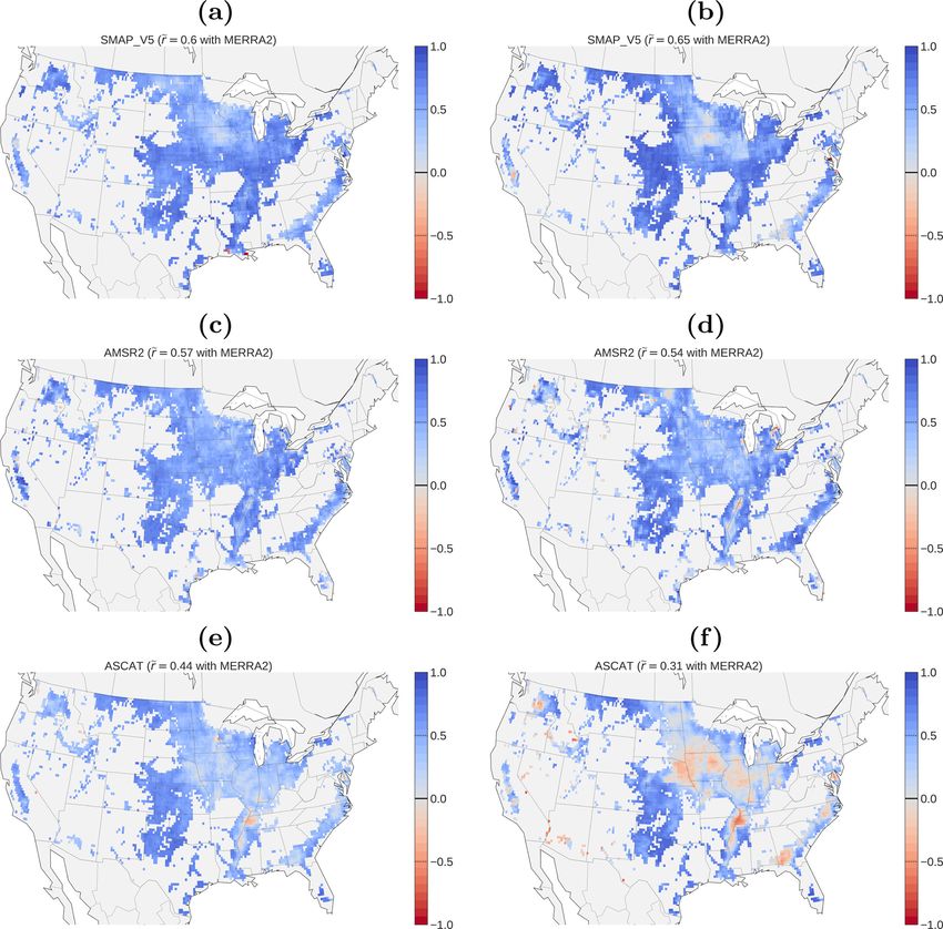
To investigate the potential detectability of IWU, we inves-
tigated the correlation between satellite and modeled soil 5.1.2 Snake River Plain
moisture during the growing season (Fig. 3). We computed
the correlation separately for dry (precipitation = 0; r dry ) and Over the Snake River Plain, ASCAT has a clear signal that
wet conditions (precipitation > 0; r wet ). If r dry is low or could be attributed to irrigation. Particularly in the central
negative over agricultural areas which are known to be ir- and westernmost areas along the Snake River, r dry depicts
Hydrol. Earth Syst. Sci., 23, 897–923, 2019 www.hydrol-earth-syst-sci.net/23/897/2019/F. Zaussinger et al.: Estimating irrigation water use over the contiguous United States 907
Figure 3. Mean correlation r between the daily time series of each satellite soil moisture product (SMAP, AMSR2 and ASCAT) and MERRA-
2 soil moisture separated for wet periods (left column; precipitation PCP > 0) and dry periods (right column; PCP = 0) during the growing
season. Correlations were calculated over agricultural areas only.
a strong negative correlation with MERRA-2, while r wet is Plains. While r wet shows weak positive correlations, r dry re-
moderately positive. Moderately negative r dry obtained for veals strong negative r, suggesting that an irrigation signal is
SMAP shows a good alignment with areas known to be ir- entailed in the ASCAT signal. However, this pattern cannot
rigated in the Snake River Plain. Although the correlation is be reliably attributed to irrigation practices as ASCAT shows
less negative than for ASCAT, the spatial pattern is resem- low correlations over the entire Corn Belt region, where agri-
bled more clearly. Here, AMSR2 shows slightly more nega- culture is generally known to be rain-fed (see Fig. 2). Vegeta-
tive r dry than r wet over agricultural land cover, but the spatial tion scattering effects from the corn canopies are a plausible
pattern appears to be less reliable than for the other satellite explanation for the observed deviation. As the corn plants
products. reach their maximum height (up to approximately 3 m) to-
wards the end of the growing season, the C-band backscat-
5.1.3 High Plains ter signal will increasingly be composed of canopy backscat-
ter and canopy-soil double-bounce reflections, while sensi-
The ASCAT product is the only one to show a distinct pattern tivity to actual soil moisture decreases (Daughtry et al., 1991;
of negative correlation over the irrigated part of the Nebraska Joseph et al., 2010).
www.hydrol-earth-syst-sci.net/23/897/2019/ Hydrol. Earth Syst. Sci., 23, 897–923, 2019908 F. Zaussinger et al.: Estimating irrigation water use over the contiguous United States
5.1.4 Mississippi Floodplain spatially distinct. Similarly, AMSR2 shows a clear signal
over the western to central Snake River Plain. Concerning
Lastly, all products show low r values over the Mississippi the Nebraska Plains, only AMSR2 IWU shows patterns that
Floodplain, although with varying magnitudes. In this region, agree with MIrAD-US. Over the Mississippi Floodplain, AS-
ASCAT shows the lowest negative correlation, followed by CAT shows the highest IWU, followed by AMSR2.
AMSR2 and SMAP. Moreover, for all SM products r dry is ASCAT-derived IWU seems to be affected by vegetation
lower than r wet . effects in the Corn Belt region and in the southeastern US.
For all sensors, the method fails to detect IWU in many ir-
5.1.5 Other regions rigated areas, especially those along the High Plains aquifer
(Nebraska, Kansas, Texas), which extends from the northern
Figure 3 also reveals that strong negative r dry (in combina- to the southern central US. A plausible explanation for miss-
tion with moderately high r wet ) based on ASCAT aligns well ing these areas is that many farmers in these regions practice
with areas known to be irrigated over the Columbia River supplemental irrigation, thus resulting in a less distinguish-
basin, Washington. As the ASCAT soil moisture product has able irrigation signal. In addition, the center pivot irrigation
a significantly higher nominal spatial resolution than the pas- systems, which are mainly used in this region, have much
sive products, we hypothesize that in this region it is the only higher water application efficiencies compared to the flood
sensor to resolve the irrigation practices. Correlations based and furrow irrigation systems used in the Sacramento Val-
on SMAP loosely agree with this pattern and AMSR2 only ley and Mississippi Floodplain (see Fig. A1). Rainfall sea-
has few valid observations over this region. In addition, both sonality is another potential reason for the underestimation
ASCAT and SMAP have patterns of r dry < r wet over an ir- in the central U.S, where the climate transitions from arid
rigated region in southwestern Georgia. In contrast, AMSR2 in the west to humid in the east. To investigate its impact,
shows moderately high positive r over this region. we plotted the average number of days per growing season
To determine the sensitivity of the growing season corre- where IWU > 0 (Fig. A3), which sums up to the number of
lation r between satellite and model soil moisture to varia- days that went into the IWU estimates shown in Fig. 4. It can
tions in fractional irrigated area within a pixel, we examined be seen that for SMAP-based IWU, a significant number of
their relationship with irrigation intensities derived from the days with irrigation (mean count) only is detected in the arid
MIrAD-US irrigated area data set (Pervez and Brown, 2010). west and southwest. For AMSR2, the mean counts are high-
However, no evidence of a negative linear relationship be- est in California, although counts in the range of 20–30 occur
tween the two variables was found (not shown), as at low irri- in the Snake River Valley, Mississippi Floodplain and other
gation fractions r is mostly dominated by effects originating agricultural regions. In agreement with the passive products,
from the remaining land cover types. Overall, the results ob- mean counts for ASCAT are highest in California and south-
tained by separately analyzing the spatial patterns of r dry and western states. There also is a clear pattern in the Mississippi
r wet between satellite and model soil moisture largely sup- Valley and along the southeastern states.
port the hypothesis that, over areas known to be irrigated, the Furthermore, the chosen global threshold of thresh2 =
remotely sensed soil moisture signal deviates from modeled 12 % also masks irrigation signals in regions where the noise
soil moisture, given that the model does not explicitly ac- level of the satellite soil moisture retrievals is rather low (see
count for irrigation (which is the case for MERRA-2). Hence, Sect. A2). Thus, a more site-specific threshold at each pixel
the overall hypothesis of this study, which is that IWU can be might lead to an improved detectability of irrigation events.
inferred from differences between the temporal variations of
the remotely sensed and modeled soil moisture, is corrobo- 5.3 Temporal behavior of soil moisture and IWU and
rated. in the four focus regions
5.2 Spatial patterns of estimated irrigation water use For a more detailed analysis on the impact of climate, crop
type and irrigation practice on the method performance, we
Spatial plots of mean annual estimated irrigation water use compared remotely sensed and modeled soil moisture time
IWU (i.e., averaged over the study period of 2013–2016) series and monthly IWU estimates at an irrigated (green
(Fig. 4a–c) suggest that all satellite products are able to iden- crosses in Fig. 2) and a non-irrigated pixel (orange crosses
tify the extensive irrigation applied in the California Central in Fig. 2) in the four focus areas (Fig. 5).
Valley. Here, SMAP-derived IWU clearly resembles the ir-
rigation patterns of the MIrAD-US data set in the northern 5.3.1 Central Valley
Sacramento Valley and southern San Joaquin Valley (Fig. 2).
The AMSR2- and ASCAT-derived IWU are generally higher At the irrigated pixel in the San Joaquin Valley, the impact
than SMAP and extend throughout the whole California Cen- of irrigation on the remotely sensed soil moisture signal is
tral Valley. Although small in magnitude, the IWU pattern evident (top panel in Fig. 5a). While MERRA-2 soil mois-
derived from ASCAT over the central Snake River Plain is ture decline in the irrigated and non-irrigated pixels reflects
Hydrol. Earth Syst. Sci., 23, 897–923, 2019 www.hydrol-earth-syst-sci.net/23/897/2019/You can also read