DEPARTMENT OF INFORMATICS
←
→
Page content transcription
If your browser does not render page correctly, please read the page content below
DEPARTMENT OF INFORMATICS
               TECHNISCHE UNIVERSITÄT MÜNCHEN

Master’s Thesis in Informatics: Robotics, Cognition and Intelligence

Biomimetic Visual Navigation: Understanding
   the Visual Ecology of Expert Navigators
           through Virtual Reality

                Jose Adrian Vega Vermehren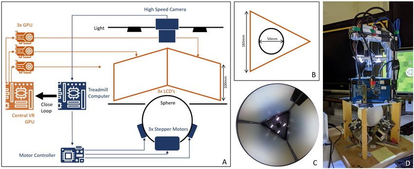
DEPARTMENT OF INFORMATICS
                 TECHNISCHE UNIVERSITÄT MÜNCHEN

Master’s Thesis in Informatics: Robotics, Cognition and Intelligence

Biomimetic Visual Navigation: Understanding
   the Visual Ecology of Expert Navigators
           through Virtual Reality

      Bionische Visuelle Navigation:
Untersuchungen der Visuellen Ökologie von
Navigationsexperten durch Virtuelle Realität

       Author:            Jose Adrian Vega Vermehren
       Supervisor:        Prof. Dr. Paul Graham | Prof. Dr. Daniel Cremers
       Advisor:           Dr. Cornelia Bühlmann | Nikolaus Demmel
       Submission Date:   10th of August 2021
I confirm that this master’s thesis in informatics: robotics, cognition and intelligence is my
own work and I have documented all sources and material used.

Munich, 10th of August 2021                                 Jose Adrian Vega Vermehren
Acknowledgments

  First and foremost, I would like to thank Cornelia and Paul for taking me again under their
wing, and letting me be part of their exciting research. I can’t wait to be back in Brighton to
do some more awesome science together.
A big thanks to Roman, Jeremy and Barbara for the additional support and feedback.
This project would not have been possible without the support of Nikolaus. Niko, thanks for
believing in me and my project when nobody else did.

   Organizing an international research project in the middle of a pandemic is no easy task. I
am very grateful to all the people who stood beside me in the process:
My parents and brother, who are always there for me.
Kai, Niki, Pablo and Felix who got me through the weirdest of times and back out into the
world. Special thanks to Felix, whose emotional support proved key in planning this project.
Charlie, Bernie and Aaron who let me believe I could achieve my goals.
Dan, Steve, Blaithin, Blake, Kostas and Matthias who are always there when I need an
alternate reality.
Munashe and Justine, without whom Brighton wouldn’t have been the same.

  Finally, I am very thankful for the financial support provided by the DAAD.
Abstract

Wood ants thrive as expert navigators in the same cluttered, dynamic, light-variant environ-
ments where most robot navigation algorithms fail [1, 2]. Virtual Reality (VR) is a novel
technique to study the visual ecology and navigation strategies of these insects [3, 4]. We
evaluate the functionality of a novel treadmill and VR system that allows experiments with
untethered walking insects [5, 6]. In a series of four experiments with incrementally complex
visual stimuli, we validate the setup and gather insights into the ants’ behaviour. The system
works remarkably well to study ant navigation, despite a few limitations. On the behavioural
side, ants use oscillations as a visuomotor control mechanisms even when deprived of sen-
sory feedback from the environment (rot. close-loop). Furthermore, ants exploit edges
as information-rich features in both simple and complex visual scenarios. Both of these
behaviours have important implications for the design of robotic navigation architectures. VR
opens a new opportunity to learn from the simple yet effective navigation strategies of ants
and design new biomimetic navigation systems.

                                             iv
Kurzfassung

Waldameisen gedeihen als erfahrene Navigatoren unter Bedingungen, in denen die meisten
Roboternavigationsalgorithmen versagen: überladene, dynamische Umgebungen mit ständig
wechselnden Lichtverhältnissen [1, 2]. Virtuelle Realität (VR) bietet eine neue Methodologie
um die visuelle Ökologie und Navigation dieser Insekten zu untersuchen [3, 4]. Wir bewerten
die Funktionalität eines neuen Systems, ein an ein VR System gekoppeltes Laufband, mit
dem laufende Insekten untersucht werden können, ohne sie zu fixieren [5, 6]. In einer Reihe
von vier Experimenten mit visuellen Reizen zunehmender Komplexität validieren wir den
Versuchsaufbau und sammeln neue Erkenntnisse zum Verhalten der Ameisen. Zur Unter-
suchung der Navigation von Ameisen eignet sich das System trotz mancher Limitierungen
bemerkenswert gut. Wir haben herausgefunden, dass Ameisen trotz mangelnder visueller
Rückkopplung (rot. close-loop) ein Oszillationsmechanismus zur visuomotorischen Regelung
anwenden. Außerdem nutzen Ameisen die potenziell informationsreichen Eigenschaften
von Kanten in einfachen und komplexen Szenen aus. Beide beobachteten Verhaltensweisen
können wegweisend sein für das Design von neuartigen Navigationsarchitekturen für Roboter.
VR eröffnet neue Möglichkeiten von den einfachen, aber eleganten Strategien von Ameisen
zu lernen, um neue bionische Navigationssysteme zu entwickeln.

                                             v
Contents

Acknowledgments                                                                                                                               iii

Abstract                                                                                                                                      iv

Kurzfassung                                                                                                                                    v

1. Introduction                                                                                                                                1
   1.1. Research Goals and Project Outline . . . . . . . . . . . . . . . . . . . . . . . . .                                                   2

2. Literature Review                                                                                                                           4
   2.1. Robot Visual Navigation Using Maps . . . . . . . . . . . . . .                                .   .   .   .   .   .   .   .   .   .    5
        2.1.1. Map-Based Systems . . . . . . . . . . . . . . . . . . . .                              .   .   .   .   .   .   .   .   .   .    5
        2.1.2. Map-Building Systems . . . . . . . . . . . . . . . . . . .                             .   .   .   .   .   .   .   .   .   .    6
   2.2. Mapless Systems . . . . . . . . . . . . . . . . . . . . . . . . . .                           .   .   .   .   .   .   .   .   .   .    8
        2.2.1. Optic Flow . . . . . . . . . . . . . . . . . . . . . . . . . .                         .   .   .   .   .   .   .   .   .   .    8
        2.2.2. Feature-Based Tracking . . . . . . . . . . . . . . . . . .                             .   .   .   .   .   .   .   .   .   .    9
        2.2.3. Appearance-Based Matching . . . . . . . . . . . . . . .                                .   .   .   .   .   .   .   .   .   .   10
   2.3. Summary: Technical and Biomimetic Navigation Algorithms                                       .   .   .   .   .   .   .   .   .   .   11

3. Methods                                                                                                                                    14
   3.1. Integration of the Treadmill and VR System            .   .   .   .   .   .   .   .   .   .   .   .   .   .   .   .   .   .   .   .   14
        3.1.1. Motion Compensating Treadmill . . .            .   .   .   .   .   .   .   .   .   .   .   .   .   .   .   .   .   .   .   .   14
        3.1.2. Virtual Reality System . . . . . . . . .       .   .   .   .   .   .   .   .   .   .   .   .   .   .   .   .   .   .   .   .   16
        3.1.3. Systems Integration . . . . . . . . . .        .   .   .   .   .   .   .   .   .   .   .   .   .   .   .   .   .   .   .   .   16
   3.2. Experiments . . . . . . . . . . . . . . . . . . .     .   .   .   .   .   .   .   .   .   .   .   .   .   .   .   .   .   .   .   .   17
        3.2.1. Wood Ants . . . . . . . . . . . . . . .        .   .   .   .   .   .   .   .   .   .   .   .   .   .   .   .   .   .   .   .   17
        3.2.2. Experimental Procedures . . . . . . .          .   .   .   .   .   .   .   .   .   .   .   .   .   .   .   .   .   .   .   .   18
   3.3. Data Analysis . . . . . . . . . . . . . . . . . .     .   .   .   .   .   .   .   .   .   .   .   .   .   .   .   .   .   .   .   .   20
        3.3.1. Data Preprocessing . . . . . . . . . . .       .   .   .   .   .   .   .   .   .   .   .   .   .   .   .   .   .   .   .   .   20
        3.3.2. Chunks and Activity Levels . . . . . .         .   .   .   .   .   .   .   .   .   .   .   .   .   .   .   .   .   .   .   .   21
        3.3.3. Individual Analysis . . . . . . . . . .        .   .   .   .   .   .   .   .   .   .   .   .   .   .   .   .   .   .   .   .   21
        3.3.4. Statistics . . . . . . . . . . . . . . . . .   .   .   .   .   .   .   .   .   .   .   .   .   .   .   .   .   .   .   .   .   24

                                                 vi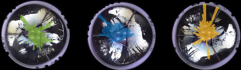
Contents

4. Results                                                                                                                     25
   4.1. Treadmill and VR Integration in Open- and Close-Loop . .                   .   .   .   .   .   .   .   .   .   .   .   25
        4.1.1. Using Ant Activity as a Metric to Filter Behaviour .                .   .   .   .   .   .   .   .   .   .   .   26
        4.1.2. Landmark Attraction in the Open-Loop . . . . . . . .                .   .   .   .   .   .   .   .   .   .   .   29
        4.1.3. Ant Behaviour in the Close-Loop . . . . . . . . . . . .             .   .   .   .   .   .   .   .   .   .   .   32
   4.2. Validating the Display of Natural Images on the VR Setting                 .   .   .   .   .   .   .   .   .   .   .   36
        4.2.1. Display of Complex Artificial Patterns . . . . . . . .              .   .   .   .   .   .   .   .   .   .   .   37
        4.2.2. Display of Complex Natural Images . . . . . . . . . .               .   .   .   .   .   .   .   .   .   .   .   40

5. Discussion                                                                                                                  45
   5.1. Evaluation of the Virtual Reality Experimental Setting .           .   .   .   .   .   .   .   .   .   .   .   .   .   46
        5.1.1. Hardware Limitations . . . . . . . . . . . . . . . .        .   .   .   .   .   .   .   .   .   .   .   .   .   46
        5.1.2. Software Limitations . . . . . . . . . . . . . . . . .      .   .   .   .   .   .   .   .   .   .   .   .   .   48
   5.2. Wood Ant Behaviour While on the Experimental Setting               .   .   .   .   .   .   .   .   .   .   .   .   .   49
        5.2.1. Open- and Close-Loop Oscillations . . . . . . . .           .   .   .   .   .   .   .   .   .   .   .   .   .   50
        5.2.2. Edge Fixation . . . . . . . . . . . . . . . . . . . . .     .   .   .   .   .   .   .   .   .   .   .   .   .   51
   5.3. Conclusion . . . . . . . . . . . . . . . . . . . . . . . . . . .   .   .   .   .   .   .   .   .   .   .   .   .   .   53

A. Appendix                                                                                                                    54
   A.1. Data and Scripts . . . . . . . . . . . . . . . . . . . . . . . . . . . . . . . . . . . . .                             54

List of Figures                                                                                                                55

List of Tables                                                                                                                 59

Bibliography                                                                                                                   60

                                                  vii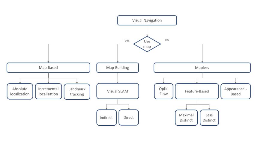
1. Introduction

From single celled organisms to mammals with complex behaviour, visual systems have
played an important role in evolution. The analogous development of light sensitive organs
has fascinated scientists since Darwin first posed his theory of evolution [7]. And not
surprisingly, behaviour is tightly intertwined: visually guided behaviour acts both as the
driver as much as the consequence of these evolving systems. Take the notorious "eagle eye"
as an example where the predator’s hunting behaviour and distinct sharp vision (a vertebrate
lens eye) evolved in synchrony [8]. Or, on an independent line of evolution, compound eyes
in insects have evolved along with remarkable control and navigation behaviours [9].
Human behaviour has also evolved strongly around vision. In fact, there is significantly
more research in vision than in any another sensory modality, up to the point that more
general concepts like "perception" or "perceptual memory" are often used synonymously to
"visual perception" and "visual memory" [10]. By no coincidence, human design of artificial
intelligence and autonomous agents reflects this tendency for vision over other modalities.
One key role for vision in natural and artificial systems is to provide information to navigation
systems. Roughly defined as finding a suitable path between the current location and a goal,
navigation is a necessary precursor for more complex behaviours [11, 12]. Robot navigation
strategies based on vision have received significant attention in the last three decades due
to the large application scope and promising results in reaching true autonomy [11]. While
contemporary visual navigation algorithms have succeeded in niche applications, navigating
the complex, undetermined, and chaotic real world remains a challenge to be solved [13].
Natural agents have clearly found solutions to the problems of navigation through complex
environments. Quite notoriously, insects have evolved vision and navigation systems strongly
constrained by their tiny brains and low visual sensory resolution. Insects are capable of
performing simple yet elegant computations to achieve their navigation tasks, e.g. foragers of
many social insect species can travel vast distances and find their way back home in the most
complex of environments [9, 14].
Ants belong to this group of expert navigators. Although ants have access to a variety of
orientation mechanisms [15], including some forms of social cues, solitary foragers rely
foremost on vision to navigate [1, 16]. Foraging ants learn the necessary visual information to
guide long and complex routes between their nest and a stable food site [17, 18]. And when
compared to artificial systems, ants have taken a different approach to solve the problem
of navigation. Contrary to map based technical implementations like visual Simultaneous

                                               1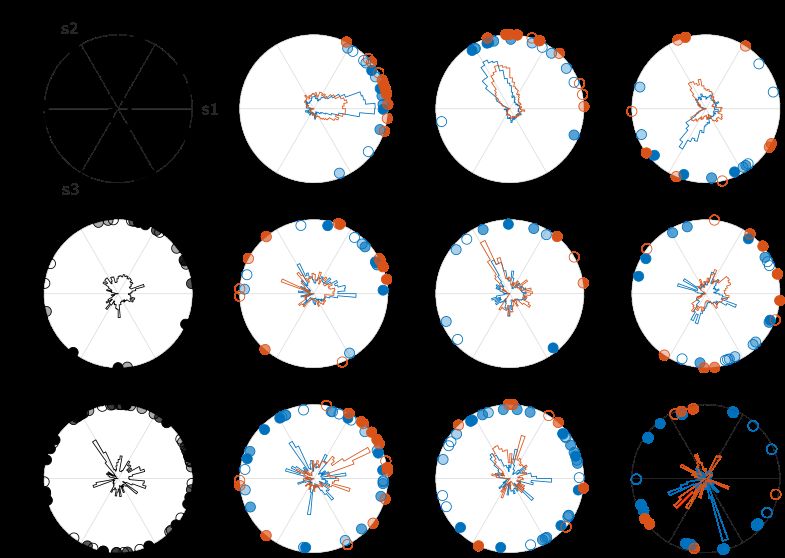
1. Introduction

Localization and Mapping (vSLAM), ant navigation is thought to be of procedural nature,
whereby ants use visual cues to trigger appropriate behaviours [1]. Furthermore, evidence
shows ant navigation to rely on the overall appearance of scenes rather than segmenting
individual visual features [19].
Although efforts to develop bio-inspired robots that mimic the ants remarkable navigation
strategies have come far, plenty of questions regarding the visual ecology and spatial memory
of the model foragers still remain unanswered [1, 20]. Research on ant navigation has
historically been limited to two approaches: field work and lab experiments. Research using
either needs to compromise between portraying foragers in their natural environments and
control over the stimuli influencing the research subjects. However, developments in computer
vision and computer graphics have created the opportunity to adapt a new technique of
experimentation: virtual reality (VR). Using VR to study the visual ecology of navigating ants
promises the best of both methodologies: absolute control over the stimuli while simulating
the ant’s natural scenery.
As a study subject, we choose wood ants. These species of ants thrives as a navigator in exactly
the kind of cluttered, dynamic and uncontrolled environment in which most robots fail to
navigate. Understanding the underlying behavioural and neuronal mechanisms involved in
their navigation could lead to a breakthrough in robot navigation.
Following this logic, this project aims to shed some light into virtual reality as a method to
study ant navigation.

1.1. Research Goals and Project Outline
The use of virtual reality as a methodology to study insects is novel, however not unheard
off. In general, most of the research in insect behaviour focuses on the common fruit fly. VR
has been extensively validated for the study of these organisms [21]. However, most of the
validated VR methodologies, including those developed for social insects [4, 3], fixate the
study specimens to a tether. This methodology significantly constraints natural behaviour.
A less invasive method requires the parallel development of a multilateral treadmill system
where walking insects can move "naturally" in response to the VR stimuli without changing
location [5]. Goulard et al. [6] recently developed such a treadmill for ant study. Under their
supervision, this project contributes to the development and validation of this system. The
following research objectives are pursued:

   1. Build upon the development of a trackball and VR system for untethered ants.

   2. Authenticate the system as a research methodology to study ant visual navigation.

   3. Evaluate the influence of a "close-loop" setting in the ant’s navigation behaviour.

   4. Describe ant behaviour when confronted with natural images in the VR setting.

                                               2
1. Introduction
To put the project into context, I begin by reviewing relevant literature (Chapter 2). The answer
to two questions summarize the outcome of this literature review: what are shortcomings of
state-of-the-art visual navigation algorithms like vSLAM, and what do previously proposed
ant navigation algorithms look like?
The outcomes of the first research goal are mainly described in the methods (chapter 3). Here
I detail upon the integration of the treadmill and VR systems as well as the implementation
of different experimental settings including a closed-loop rotation system.
The results in chapter 4 are divided into two sections: (i) validation of the system to investigate
ant navigation and (ii) ant navigation in complex VR scenes. Research goals 2 and 3 are
explored in the first part. Using two sets of experiments with a simple visual cue, I describe
and compare ant navigation on the open- and close-loop system. Research goal number 4
is detailed in the second part; here, I describe ant navigation on the novel system with a
complex artificial and a complex natural scene.
Finally, a discussion over the results is offered in chapter 5. Here I reflect upon the four
research goals and summarize the validity of the novel system to study ant navigation.
Furthermore, I describe follow-up experiments that could eventually lead to a new robot
navigation algorithm inspired by ants.
32. Literature Review
Both natural and artificial agents rely on spatial memory to navigate, i.e. agents need to
remember information about their surroundings in order to be able to return to that specific
location. Navigation using vision is the primary modality for both expert animal navigators
and state-of-the-art robot navigation algorithms [11, 9]. That being said, visual spatial
navigation varies in complexity. We distinguish four levels of cognitive complexity [22]. In
increasing order:
1. recognition of a location upon re-encounter
2. visual servoing towards a clear visual cue at the destination
3. visual homing, i.e. comparing a stored "home" view to guide the agent back to its "base"
4. linking visual information to a "map-like" representation of space
Even the simplest of these visual recognition tasks, challenges agents to deal with all sort of
visual problems [22, 13]. Breakthroughs in computer science have advanced robot navigation
significantly. Even so, navigation in certain locations, e.g. cluttered, dynamic, outdoor
environments, remain unconquered. And yet, ants and other social insects thrive as navigators
under these conditions; evolution seems to have found clever solutions to many of these
visual problems [9].
In order to explore new strategies for visual navigation, it is important to understand the
limitation of previous approaches. This chapter systematically explores the most important
techniques in visual navigation. Both technical algorithms and biologically inspired models
are categorized by their strategy. The main drawbacks of each approach are outlined. Figure
2.1 offers an overview over the categorization.
In literature, we find a distinction between indoor and outdoor navigation [23, 11]. The latter
is then divided in structured (e.g. roads) and unstructured environments. However, if we
ignore methods involving an external reference frame (e.g. GPS), outdoor navigation shares
similar constraints with its indoor counterpart. This thesis focuses on this set of application
scenarios and thus treats outdoor navigation as a complex, less controlled version of indoor
environments.
Based on the available information and strategy, visual (indoor) navigation algorithms can be
roughly divided into three categories: mapless systems [24], map-based systems and map-
building systems (Fig. 2.1; [23, 11, 25]). While mapless systems vary in cognitive complexity
42. Literature Review
Figure 2.1.: Overview vision-based navigation methodologies. Adapted from [25].
(levels 1-3), the latter two use maps, and thus fall into the highest level of cognitive complexity
(level 4).
2.1. Robot Visual Navigation Using Maps
Increasing developments in computer vision have made vision based navigation specially
effective to pursue robot autonomy. In the last three decades, countless research efforts have
been made to improve their navigation algorithms. Most approaches are based on the use of
maps. Depending on the task and the previously available information, agents can employ
map-based or map-building systems [23, 25].
2.1.1. Map-Based Systems
Map-based systems require a predefined spatial layout of the environment. The data structure
and detail varies from a full CAD model to a simple graph, depending on the system [24].
At its core, the map is used to generate a sequence of expected landmarks while the vision
system attempts to locate them. A successful match allows the robot to self-estimate its
position in the map relative to the recognized landmark. Hence, navigation using this method
is a sequence of four steps: (i) image acquisition, (ii) landmark detection, (iii) matching of
expectation, and observation and finally (iv) position estimation.
The complexity of these systems lies mainly in the third step, matching (correspondence
problem). Different approaches to solve it have been proposed [24, 23]:
52. Literature Review
Absolute Methods The system does not know the starting position of the robot. Hence, an
exact match between features is required to locate the agent within the map (correspondence
problem).
Incremental Methods These algorithms keep track of the localization uncertainty starting
from a known position. Hence, an exact match is only needed to recalibrate the error
propagation. The matching problem is reduced to a probabilistic analysis.
Landmark Tracking The general idea is to trace known landmarks matched at a known
starting position across subsequent frames. Here, landmarks can be either natural or artificial
and need to be defined by a human operator.
Map-based system are quite successful to solve tasks in known and well-defined environments.
However, they are strongly affected by certain limitations [24, 23]:
• Prior knowledge of the environment in the form of a map is needed. Without an addi-
tional obstacle avoidance systems, they are unable to navigate dynamic environments.
• Ambiguities in matching increase the complexity and reduce the systems’ robustness.
Map-based systems are unsuitable to navigate cluttered, chaotic environments.
2.1.2. Map-Building Systems
Map-building systems have received the highest attention in recent years. Compensating
one of the main drawbacks of map-based systems, map-building systems navigate the
environment, while building a representation of it. Although other methods exist, by far
the leading strategy, is Simultaneous Localization and Mapping (SLAM). These systems are
able to navigate unknown environments by performing three activities in parallel, navigation,
mapping and localization [24, 23, 2].
Vision based SLAM (vSLAM) algorithms have been greatly developed in the last thirty years,
and are currently considered the state-of-the-art approach for visual robot navigation. Hence,
a more detailed analysis of the strategies employed, and their shortcomings, is in order:
vSLAM Methods
With the rapid development in camera technology, camera sensors have become cheaper, they
consume less power and are able to provide robust and highly detailed real time information
of the environment. vSLAM algorithms rely solely on cameras as their navigation sensor;
significantly increasing the range and flexibility, not to say affordability, of their application
domain. Nevertheless, compared to other approaches that use different sensors (e.g. Lidar),
vSLAM algorithms come with a higher technical difficulty due to the limited field of view [2,
62. Literature Review
26].
vSLAM works in four modules. In the first module, the sensor data is retrieved and pre-
processed. Next, the Front-End module uses the image motion to generate a first estimate
of position. In parallel, a system called Loop Closure uses the preprocessed sensor data to
calculate the similarity between the current image and a stored map representation. The third
module, Back-End, constraints the initial estimation from the Front End with the information
from the Loop Closure. Finally, the Back-End solves an optimization problem between the
last module, Map, and its current global estimate of the agent’s position [2].
Based on the method employed by the Front-End, vSLAM algorithms are divided in two
categories: indirect and direct methods [2, 25]:
Indirect methods Indirect Methods are based on the assumption of geometric consistency.
Instead of using entire images, algorithms in this category use geometric features to estimate
the image motion. A feature should be invariant to rotation, viewpoint and scale changes, as
well as robust against noise, blur and illumination. These feature points need to be extracted,
matched and estimated. The first step, feature extraction, is a computational expensive
operation, hence the success of the algorithm relies heavily on the speed and quality of
feature extraction (feature extraction problem). SIFT is the most used extraction method (see
section 2.2.2 for more detail). Like with absolute map-based systems, matching is also an
important issue, heavily constrained by mismatches and moving targets (correspondence
problem).
Furthermore, the density of distinct points that the algorithm can reconstruct has a strong
influence on the application domain; indirect methods do not perform well in cluttered
texture-less environments [2, 25].
Direct methods Direct methods are based on the greyscale-value invariance assumption:
a pixel has the same greyscale value in subsequent images. Hence, the direct method does
not extract individual features, but uses all the information in the image to estimate image
motion. Algorithms under this category are more robust to geometric changes. They are in
general faster and are better at dealing with dense maps. The achievable density of these
maps is proportional to the available computational power. Nevertheless, these algorithms
are sensitive to direct sunlight and shadows, illumination variance and specular reflections [2,
25].
Hybrid methods Hybrid methods attempt to increase efficiency by exploiting each of the
previous methods at its strongest. They first employ indirect methods to initialize feature
correspondence and then turn towards direct methods to refine the camera poses [25].
72. Literature Review
Challenges of vSLAM
Although vSLAM algorithms have come a long way, plenty of challenges remain to be solved.
Mainly, how to robustly navigate more complex environments while meeting the requirements
of real-time agents [27, 2]:
• vSLAM algorithms are still not very good at dealing with dynamic environments.
Moving elements in a robot’s surrounding significantly complicate feature matching
and generate unwilling changes in illumination.
• Texture richness is important. Indirect methods perform poorly in texture-less environ-
ments. Furthermore, regular patterns can cause mismatches and missing features.
• Variance in illumination violates the underlying assumption of direct methods. It has
jet to be solved for dynamic scenarios and refined for static ones. Intense sunlight and
shadows, as well as reflections common in uncontrolled outdoor spaces, can cause the
system to fail.
• The complex computations required to match camera poses and find a global optimum,
constraints to the size and speed of agents running vSLAM algorithms.
• Scarcity influences the precision during navigation and the quality of the arising maps.
There is a trade-off between density and computational power.
• Mismatches by the Loop Closure detection have the potential to limit the system’s
robustness and fail navigation in both dynamic and static environments.
2.2. Mapless Systems
As established before, keeping a "map-like" representation of space requires the highest level
of cognition (level 4), i.e. relying on maps (either prebuilt or built during navigation) is an
expensive strategy with a strong influence on performance. And yet, evidence suggests that
social insects are able to perform complex navigational tasks without the use of cognitive
maps [28]. Here, I shall hence focus on the next most complex cognitive ability, homing (level
3).
Systems in this category are relatively new compared to the previously described ones.
This section reviews the most important technical and biomimetic approaches to mapless
navigation. Special emphasis is made on insect-navigation models and algorithms.
2.2.1. Optic Flow
Optic flow (OF) is a strategy employed both by humans and animals. Agents use the motion
of the surface elements in the environment to calculate a moving direction and the distance
82. Literature Review
to obstacles [24]. Speed and accuracy can be regulated according to the task at hand. Bees,
expert navigators, are known for their mastery of this strategy. These insects are able to
regulate flight direction, speed and height as well as avoid obstacles and calculate odometry
with little more than optic flow calculations [9].
Already in 1993 Santos-Victor et al. [29] proposed an optic flow algorithm inspired by the
bee’s flight strategies. Here, localization is achieved by comparing the image velocity of both
eyes (i.e. cameras). If both sides move at the same speed the agent keeps moving forwards,
however if there is a difference, the robot steers in the direction of lower speed.
Robots implementing optic flow as a navigation strategy face two important challenges: (1) OF
cannot disentangle distance from velocity, and (2) OF is very small and thus less descriptive
in the direction of flight [30]. De Croon, De Wagter and Seidl [30] recently proposed a method
that treats optic flow as a learned and not innate feature. Their robot achieves smoother
landings, better obstacle avoidance and higher speeds by implementing a previous learning
process.
Homing based on Optic Flow OF is a powerful tool for steering and object avoidance. It
is however often underestimated as a method of spatial memory. Vardy and Möller [31]
proposed in 2005 a series of techniques based on insect homing that allow corresponding two
images by means of optic flow. They show multiple methods, including block matching and
differential OF as plausible models of efficient insect homing. The simplicity and robustness
of these methods and their propensity for low-frequency features are ideal for lightweight
robot navigation.
2.2.2. Feature-Based Tracking
Equivalent to its map-based and map-building counterparts, mapless feature-based methods
also track the relative changes of previously extracted features across subsequent images.
Since in this case no map is involved, a learning step, where the agent remembers its
surrounding in the form of snapshots at the home location, is required [24].
A feature is a landmark that can be clearly segmented from the image’s background. First,
the agent must extract the same feature in both the current image and snapshot (feature
extraction problem). Then, each feature has to be matched in the current and remembered
image (correspondence problem) [24]. Extraction approaches vary on the level of landmark
uniqueness, while some methods strive for maximal distinctive features, others use less
unique features [31]:
Maximal Distinct Features
Algorithms in this category strive to extract maximally distinct features. The ideal feature is
unique to the point, that it can be corresponded with 100% accuracy, i.e. there is no other
92. Literature Review
feature that could look like that. The computer vision algorithm SIFT stands out for its
popularity and performance:
Scale Invariant Feature Transform A milestone in feature extraction was the invention of
the scale invariant feature transform (SIFT) algorithm [32]. SIFT is nowadays a standard
method in landmark detection, both for map-building and mapless technical systems alike.
In a series of image operations, SIFT extracts features invariant to scaling, rotation and
illumination, significantly increasing robustness to matching upon re-encounter.
In order to establish one-to-one correspondences, distinct feature methods have to search for
the landmark in the whole image. Since the entire image is searched through anyway, no
preprocessing steps like image aligning are needed. That being said, distinct features are
hard to extract in cluttered environments. Furthermore, the extraction and matching process
are both computational expensive and a trade-off between computation speed and onboard
load has to be made for autonomous agents [24].
Less Distinct Features
Less distinct features are significantly easier to extract, matching, however, is often ambiguous.
One of the first models of insect navigation falls into this category:
The Snapshot Model Most insect navigation research and many robot navigation algo-
rithms relate to the snapshot model. Based on landmark navigation experiments with bees,
Cartwright and Collet [33] described a homing method capable of deriving a heading direc-
tion from the discrepancies between a single snapshot and the current image. Less unique,
dark and bright features are used to navigate. The difference between snapshot and current
image is used to generate a relative movement vector. By iteratively lessening the mismatch
between features, the agent is able to navigate back home.
When using non-unique features, many correspondences might exist. To solve this problem
with reliability, the agent needs to align the current view and the snapshot view to a common
coordinate system. The implications are both unpractical and biologically implausible, which
is why follow-up research has focused on methods of alignment matching [31].
2.2.3. Appearance-Based Matching
In its core, appearance based methods store representations of the environment and associate
them with the correct command to steer the agent to its goal [24]. It is a two-step approach.
First, the agent has to learn prominent information of its surrounding and attach the appro-
priate steering information to it. Afterwards, during navigation, the agent has access to the
correct steering command upon re-encounter with a previously learned template. Different
102. Literature Review
methods employ different sources of information to describe unique locations. Two strategies
derived from ant navigation are worth highlighting:
Image Warping The warping method, initially proposed by Franz et al. [34], has proven its
value by multiple robotic implementation as a robust homing strategy. The general idea is to
compute the set of all possible positions and rotations between the current location and the
goal. The current image is distorted (warped) to approximate the view the robot would have,
had it moved according to the corresponding parameters. The warped image can then be
compared with the snapshot by a similarity measure. Homing is achieved by an exhaustive
search for the parameters that generate the most similar warping.
The robustness of this method makes it a very reliable navigation strategy. Nevertheless, the
cognitive complexity grows exponentially with the space of possible parameters, making it
unsuitable for lightweight navigation in complex environments.
Image Difference Function The homing algorithm presented by Zeil et al. [35] is surpris-
ingly simple yet effective. The home location is saved as an omnidirectional image. The Image
Difference Function (IDF) calculates the pixel-wise similarity (root-mean-square) between the
current image and snapshot. In natural images, the difference increases monotonically with
distance from the home location, so gradient descent can be used to determine a heading
direction. To address the image-align problem, compass information can be abstracted from
an equivalent gradient in the rotation Image Difference Function (rIDF).
Although successful in both indoor and outdoor experiments, this strategy is limited by a
certain distance from the home location, within which, a global minimum of the function
exits (often called catchment area) [36]. Further research has shown, that the catchment area
can be significantly expanded by stitching views together and forming routes [37, 38, 39].
2.3. Summary: Technical and Biomimetic Navigation Algorithms
Navigation is a complex task that agents need to master to achieve true autonomy. This
chapter reviews some of the most influential approaches to visual navigation proposed in
the last 30 years. Table 2.1 shows an overview of the different methodologies and their main
drawbacks.
Certain ideas and strategies stretch across the presented categories. A comparison of the
limitation of each methodology leads to certain conclusions:
• Navigation with a map is an anthropomorphic notion. Social insects are an example
of how complex navigational tasks can be achieved without them. Prebuild maps are
just not practical, and building a map during navigation is an expensive luxury. The
procedural nature of mapless strategies is simple yet effective.
112. Literature Review
Table 2.1.: Overview of the reviewed algorithms.
Method Category Strategy Main Drawback(s)
Absolute Map-based Exact feature match Map needed, robustness
Incremental Map-based Uncertainty propagation Map needed
Landmark Tracking Map based Known landmark match Landmark design
Indirect vSLAM Geometric consistency Texture, map scarcity
Direct vSLAM Greyscale-value invariance Lightning variability
Hybrid vSLAM Direct and Indirect vSLAM Comp. complexity
Correspondence OF Mapless Optic Flow Robustness
SIFT Feature-Based Maximal distinct features Comp. complexity
Snapshot Model Feature-Based Indistinct Features View alignment
Image Warping Appearance-Based Image Distortion Comp. complexity
IDF Appearance-Based Pixel-Wise Similarity Catchment area
• Across categories, methodologies relying on geometric features (indirect vSLAM, feature-
based mapless) are faced with the feature extraction problem. Robust navigation requires
these features to be scale, rotation and illumination invariant. Feature extraction
algorithms like SIFT are computational expensive and perform poorly in cluttered,
texture-poor environments. Systems that employ less distinct features (Snapshot Model)
perform better under these conditions, but are unpractical due to the image-alignment
prerequisite.
• Using the information encoded in the entire image instead of single features leads to
more robust algorithms (direct vSLAM, appearance-based mapless). A good metric for
image similarity are pixel-wise comparisons. The image attribute used to describe a
location varies across methods. One of them, photometric comparison, is susceptible to
extreme lighting conditions. Optic flow is another source of information that can be
exploited to describe a location. The IDF strategy shows promising results, and it has
been shown that bigger catchment areas can be achieved by stitching multiple views
together.
Mapless, appearance-based strategies are both biologically plausible models of insect nav-
igation and efficient solutions for robot navigation. Current robotic implementations of
these techniques still struggle under certain environmental conditions: cluttered, dynamic,
light-variant sceneries. Wood ants have adapted to navigate under precisely these conditions.
122. Literature Review
Yet, we know little about the visual ecology of these expert navigators. In other words, we
have a good model on HOW ants (and robots) can use visual information to navigate, but
still need to understand WHICH information in their natural panorama plays a decisive role.
New research methodologies are needed to explore this question.
133. Methods
Our VR/treadmill system provides a novel technique to investigate the visual ecology of wood
ants. This chapter deals with the methodologies involved, and is divided in 3 sections. First, I
describe the integration between the treadmill and VR systems. I report the functionality and
limitations of the experimental setup. Next, I describe the experiments we performed. We
collected four datasets, divided in two groups: (i) with a simple visual cue, and (ii) with a
complex scene. These groups correspond to the two main sections of the results (Chapter 4).
Finally, I describe the tools and methods used to analyse the data on each of the four datasets.
3.1. Integration of the Treadmill and VR System
The system is composed of two subsystems, the motion compensating treadmill and the VR
setting. In a previous publication, Goulard et al. [6] documented the treadmill subsystem
extensively, however at that stage of the systems’ development, the VR system had not yet
been developed. In this section the functionality of the experimental setup and the new
integration between both subsystems is described. Figure 3.1 offers an overview of the
complete experimental setting.
3.1.1. Motion Compensating Treadmill
The motion compensating treadmill works through an information loop (3.1A blue, [6]). The
ants are positioned on top of a white foam sphere with a diameter of 120 mm. Aligned to the
centre of the sphere, a high speed zenithal camera (Basler ace acA640-750 µm – monochrome)
tracks the movements of the ant. The camera is positioned 150 mm above the sphere and
is equipped with a 12 mm focal lens objective. External lighting is provided by four lights,
each consistent of three white LEDs and a diffusive cover. The lights are supported by
a white cardboard plane that blocks external visual stimuli. The camera communicates
with a Raspberry Pi (4 Model B) microcontroller (running Ubuntu 17), which serves as the
computation unit of the treadmill system. Here, the motion of the ant is computed into a
compensating motor signal and forwarded to the motor controller via USB. An Arduino Uno
microcontroller connected to 3 motor drivers (STMicroelectronics, ULN-2064B) controls the
rotation of the rotors. The three stepper motors (SANYO SY42STH38 - 0406A) are equally
distributed around the sphere and tilted by 60 deg. Each one is equipped with a dual disc
143. Methods
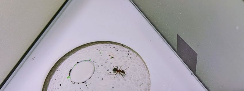
Figure 3.1.: Experimental Setting. (A) Information flow between systems: treadmill subsystem
(blue) and VR subsystem (orange). The black arrow symbolizes communication in the close-
loop condition. (B) Top view. VR system is composed of three screens arranged in an
equilateral triangle around the trackball. (C) Panoramic picture from inside the VR chamber.
The horizontal lines of the displayed visual elements are distorted to accommodate the
system’s geometry and appear as projected equidistantly from the ants’ perspective. (D)
Picture of the experimental setup.
omni wheel (aluminium, diameter: 60 mm, 2 discs, 5 rollers/ disc) to avoid creating friction
when the ball has to rotate perpendicularly to the axis of the rotor. The compensation signal
is carried out by the three motors to rotate the sphere and keep the ant at the centre of the
ball. A white board covers the space around the top of the sphere (5 cm) and supports the
three screens of the VR system. A small webcam is additionally fitted to the cardboard ceiling
and allows the experimenter to look inside the chamber without disturbing the ant.
Motion Tracking
The position and orientation of the ants are tracked every 700 frames−1 . The exposure time
is set to 1000µs. A custom Python program developed by Goulard et al. [6] and slightly
modified by me is used. Each frame is binarized using a threshold of 50% and reversed such
that the ants appears as a white "blob" in a black background. Based on previous frames
and size, an ellipse is fitted around the contour of the blob that most likely represents the
ant. The centre and orientation of the ellipse are calculated. The orientation is approximated
with a ±180 deg uncertainty, which is resolved in post-processing by assuming the ant moves
forwards, and kept consistent by minimizing the heading change between two consecutive
frames. The initial orientation is determined by the experimenter by looking at the ant though
the webcam and "flipping" the orientation in case of a mismatch. Sudden movements of the
153. Methods
ants might cause a mismatch in orientation further into the trial. These are addressed in the
data analysis.
Controller
The x and y position of the ant, estimated from the centre of the tracked ellipse, are used to
actuate the motors and keep the ant in the centre of the sphere. The system employs two pro-
portional derivative (PD) controllers, one for each coordinate. For a detailed implementation
of the controller, see [6]. The only change from the previous implementation of the system
are the control parameters. After mounting the VR and treadmill system together, I manually
optimized the proportional and derivative gains (K p = 1, Kd = 0.05). The control feedback
loop is kept at a frequency of approx. 500 Hz.
3.1.2. Virtual Reality System
The VR system (Fig. 3.1A and B orange) is composed of three LCDs (WINSTAR TFT-LCD
Module 7") with a resolution of 800x480 px. The screens (165x100 mm) are mounted on the
white board around the sphere, forming an equilateral triangle. Each screen is powered
independently and connected via HDMI to its individual graphics process unit (GPU). All
three screen-GPUs connect via micro-USB to a central GPU running Ubuntu 17. The VR
computer runs a custom python program developed by Goulard et al. [40] and slightly
modified by me. The communication between the GPUs is coordinated by an instance of
the Robot Operating System (ROS); the central VR GPU serves as master and the individual
screen-GPU’s subscribe to it.
The VR system supports the display of simple visual shapes and natural panoramic images.
Regardless of the input, the displayed visual elements are distorted to fit the screen geometry,
i.e. as the image elements move towards the corners, the horizontal lines are scaled dispropor-
tionally to accommodate for the change in perspective. Hence, from the centre of the sphere,
the visual elements all look as if projected equidistantly. Figure 3.1 shows the result of the
distortion on the example of a black rectangle on one of the corners.
The system is also able to display panoramic images. These are first unwrapped (black
pixels are used to fill up empty space) and then distorted to accommodate for the change in
perspective. The system is able to display full colour images, nevertheless for the experiments
presented in this thesis, we transform the images into black and white (Fig. 3.3).
3.1.3. Systems Integration
The treadmill and VR systems communicate using ROS. The treadmill computer serves as
ROS-master, and the VR computer subscribes as a listener. This way both systems stay in
synchrony. The experimental conditions, i.e. type and duration of visual display, are defined
163. Methods
by the VR system. This one remains in standby until a new "trial" is started globally by the
treadmill system. Communication happens at a rate of approx. 65 Hz. At each time step, the
treadmill system communicates the estimated heading direction of the ant to the VR system.
Two important data outputs are generated. The treadmill outputs the angular velocity of the
sphere at a rate of approx. 113 Hz and the VR system outputs the heading direction of the
ant at a rate of approx. 65 Hz. The timestamp of each data entry is synchronized by the ROS.
System Open- and Close-Loop
The integration of both systems allows to manipulate the feedback loop between the ant and
its environment. From a systems’ perspective, the natural condition of the world is open-loop.
This means that the ant has an influence on how she perceives the environment by moving,
e.g. when the ant rotates clockwise, the visual features appear to rotate anti-clockwise. This
is an example of a rotational open-loop. In translational open-loop, when the ant moves
towards an object, the projection of the object on the ants’ retina grows.
In its current stage of development, the VR system is not yet capable of simulating a
translational open-loop, i.e. when the ant moves towards a black rectangle, the display size of
the rectangle stays the same. Hence, our system is constantly in translational close-loop.
For rotation, the system offers the possibility to change between open- and close-loop. If a
visual stimulus stays at the same position on the screen, the system is simulating the natural
open-loop condition. However, if we rotate the visual stimuli on the screens by the same
amount and direction as the ant rotates, then the system is in close-loop and the ant has no
control over what she sees. This is a powerful tool to analyse the neuronal circuitry of the
insects. To achieve this condition, the VR system takes the estimated orientation of the ant
communicated by the treadmill and rotates the displayed stimulus accordingly.
3.2. Experiments
To test the functionality of the system and learn more about the visual strategies employed by
ants, we designed two groups of experiments. All the experiments were carried out at the
University of Sussex in Brighton, UK.
3.2.1. Wood Ants
We work with wood ants (Formica rufa) that are kept in the laboratory (Fig. 3.2). The colony
was collected from woodland (Broadstone Warren, East Sussex, UK) and is housed in large
tanks in a lab with regulated temperature of 20-25°C. Water, sucrose and dead crickets are
provided ad libitum on the surface of the nest. Ants are kept under a 12 h light to 12 h dark
cycle. During the experiments, the food supply is kept at a minimum in order to increase
173. Methods
Figure 3.2.: Wood ant. Image shows a forager of the species Formica rufa standing on the
trackball while facing a black bar as a unique visual cue in an otherwise white environment.
foraging motivation. Water access remains constant.
During an experiment, we are mostly interested in ants with a strong motivation to forage.
To only select "motivated" ants, we position a small plastic box without lid on the surface of
the nest. Motivated foragers climb inside the box. The inner walls are painted with a fluon
solution, so the ants can not climb back out. Only ants that pass the "box-test" are tested on
the VR system.
Ant Marking
In some experiments, individual ants are tracked across multiple trials. Between each trial,
the ants are returned to their nest momentarily. In order to differentiate them, ants in these
experiments are marked. We use acrylic paint in different colours to mark the thorax and
abdomen of the ants with a tiny drop of paint. Through a colour code, we are then able to
identify individuals.
3.2.2. Experimental Procedures
The general procedure to test the ants is constant across all trials. After depositing the ant
on the surface of the trackball with a plastic flag, the experiment is started. Within the first
30sec, the experimenter determines if the heading orientation is being tracked correctly, and
otherwise flips it with a keyboard command. The ant stays on the treadmill until (i) the time
is over (either 3 or 10 min), (ii) the experimenter notices that the ant tracking flipped the
heading direction, or (iii) the ant escapes the treadmill. In any case, the tracking is stopped,
and the ant is collected. Trials that incidentally stop in the first 30% of the total time are not
saved. In these cases, the same ant is tested again.
183. Methods
Experiment Conditions Trials Time Frame
Open-loop C20: s0, s1, s2, s3 43 27-29.04.2021
Open-loop C20: s1, s2, s3 26 13.07.2021
Open-loop C40: s1, s2, s3 45 14-16.07.2021
Close-loop 0, ±30 offset 69 21-22.04.2021
Close-loop ±20 offset 31 12-13.07.2021
Close-loop ±10, 40 offset 64 17-19.07.2021
Artificial Pattern A1, B2, A3, B4 95 09-11.06.2021
Natural Image A1, B2, A3, B4 74 13-14.05.2021
Natural Image A5 13 18.05.2021
Natural Image B1, C1 35 13-14.05.2021
Table 3.1.: Overview of recording days and sample sizes for all four datasets.
Experiments with a Simple Visual Cue
Two datasets with a simple visual cue were collected: open- and close-loop. Both follow the
same experimental procedures. A simple black rectangle is used as a unique visual landmark
in an otherwise white environment (Fig. 3.2). The size of the cue is of 35 deg high and
20 deg wide. The close-loop dataset uses an additional experimental condition where the cue
dimensions are altered to 35x40 deg. All the experiments in this group last a maximum of
10 min. In this group, only naive ants are tested. Table 3.1 provides an overview of the test
dates and sample sizes.
Experiments with a Complex Pattern or Image
In order to test the VR’s ability to display complex visual stimuli, as well as explore the visual
ecology of wood ants, two datasets were collected: artificial pattern and natural image. Both
have similar experimental procedures. In this group, we test individual ants multiple times
(see Ant Marking). The marked ants are returned to their nest after each trial for approx.
3 hours. In the natural image experiment, the fifth and last trial is conducted four days later.
Table 3.1 provides an overview of the test dates and sample sizes.
Artificial Pattern The visual stimulus used in this dataset is a panoramic pattern of black
rectangles (Fig. 4.11). The rectangles are organized in groups. There are three groups: one
wide rectangle, two middle-sized rectangles and four thin rectangles. The height of all bars is
the same. The panoramic pattern was designed in Cartesian coordinates and wrapped into
polar coordinates using an external function (MATLAB 2021a, PolarToIm(img, 0, 1, 1024, 1024)
[41, 42]). The polar pattern is then fed into the VR system. This process is followed for each
rotation of the pattern.
193. Methods
Figure 3.3.: Natural woodland image. (A) Raw image in original rotation, (B) image from
A rotated by +90 deg and transformed to black and white. (C) Picture from inside the VR
chamber with condition C, which is image A rotated by -90 deg.
Natural Image For this dataset we use a panoramic picture taken in the woods (Abbots
Woods, East Sussex, UK) using a fish-eye camera (Kodak SP360 4K). We selected the image
for its texture richness. The raw picture is rotated according to the desired condition (A, B,
C). We binarize the pictures before feeding them into the VR system. Figure 3.3 shows each
of the steps.
3.3. Data Analysis
For the entire data analysis, I use MATLAB [41]. The data outputs (see 3.1.3) for each trial are
saved in .csv format and imported into MATLAB. In total, four datasets were collected, namely:
open-loop, close-loop, artificial pattern and natural image. Each is analysed independently.
3.3.1. Data Preprocessing
As described before, one of the shortcomings of the tracking system is the inability to dif-
ferentiate between the head and tail of the ant, leading to an ±180 inaccuracy. To deal with
this, at the beginning of each trial the experimenter flips the heading direction manually in
case of a wrong head-tail match (happens in 50% of the trails). During the trial, the treadmill
system assumes a minimal change in heading direction between two frames and hence keeps
this one constant. Nevertheless, if an ant makes a very sudden turn or stands on its hind
legs (reducing the ellipse shape to a circle), the ant-tail matching might fail again. These are
ant-induced flips (happens in about 10% of the trials), and the data afterwards is not useful
any more.
All datasets undergo the same preprocessing step. Based on the recorded heading direction, I
calculate the angular velocity each 0.2 seconds. A threshold in the angular velocity is manually
fitted to each dataset to identify strong sudden changes in heading direction, i.e. a flip either
manually induced by the experimenter at the beginning or by the ant due to a strong sudden
203. Methods
movement (close-loop: threshold = 455 deg/second, all others: threshold = 750 deg/second).
A correction induced by the experimenter at the beginning needs to happen within the first
60 sec. Data before this flip is cut off. Any subsequent flip outside this time fame is considered
ant-induced, and the data after the flip is cut off. Hence, only data after the human correction
and before an ant-induced-flip, is considered further. Finally, the total recording time after
the cuts needs to be greater than 10% of the experiment time, trails that do not match this
criterium are discarded.
Afterwards, all heading angles are rotated by 90 deg to accommodate to the system’s coordi-
nate system, which has a zero value at the centre of screen one and positive angular velocities
in counterclockwise rotations.
3.3.2. Chunks and Activity Levels
I use the activity of the motors as a metric to segment ant behaviour. The underling
assumption is the following: ants are attracted to visual landmarks. When an ant moves
towards a landmark, it will decrease its angular speed and increase its forwards speed. A
high forward speed on the treadmill is reflected in a high (counter) speed of the trackball.
Hence, the level of ant attraction is proportional to the rotation velocity of the trackball.
To exploit this, I segment the motor angular velocity data into chunks of uninterrupted
activity. Figure 3.4 illustrates the chunk extraction process. First, I sum the x (A) and y
angular velocities (Θ̇ x and Θ̇y ) and take the absolute (B). Each data entry is then classified into
a quadratic scale, assigning each entry a value between one and four based on the strength
of the signal. To encode the density of the signal, I calculate the average value over a 2 sec
widow (C). Here, all values under 0.05 are rounded down to zero. The resulting step function
encodes both the density and the amplitude of the signal. I smooth this function using a
moving median and a window of 1000 entries (D).
The smoothed step function is divided into chunks. A chunk is a period of time within which
the step function never reaches zero. For each chunk, I determine the integral under the step
function. Integrals under a value of 100 are discarded as noise. All other integral values
(one per chunk) in a dataset are pooled together, and the quartiles are calculated. I use the
quartiles as boundaries and assign each chunk an activity level between one and four (E).
Since the treadmill and VR data are synchronized, I can take the time interval of each chunk
and apply the same division to the ant’s heading data. The activity level, which is soley based
on motor activity, is kept. As an end result, I have the ant’s heading direction data segmented
and categorized into activity chunks (F).
3.3.3. Individual Analysis
Although the overall analysis of the data followed the same methodologies, in each dataset I
performed some specific manipulations in the data. This section gathers these techniques.
213. Methods
Figure 3.4.: Activity chunks extraction process. Motor angular velocity in blue, ant angular
velocity in grey. (A) Raw motor angular velocity in x direction (Θ̇ x ). (B) Absolute sum of Θ̇ x
and Θ̇y . Thresholds used to sort data in next step. (C) Motor activity divided in four levels
according to amplitude. Density of the signal is encoded by the average amplitude in a 2 sec
window. (D) Contour of the smoothed motor activity. Data is divided into chunks within
which the motor activity does not reach zero. (E) Motor data (same as B) with the extracted
chunks. The integral under the contour of each chunk is calculated and divided into one of
four quartiles of activity. (F) Angular velocity of the ant with the chunk divisions and labels
calculated on the base of motor activity.
Circular Histograms
For all circular histograms presented in the results, I use the polarhistogram() function with a
bin size of 5 deg and a normalization set to probability. The mean and variance values of all
circular data are calculated using the circular statistics toolbox [43]. All histograms within a
dataset are scaled by the same factor. The dots on the outer rim of the plot have the mean
angle for an individual ant or chunk and are colour coded to represent the relative variance of
that mean. To do this, I pool together the variance value of all ants in that condition, calculate
the quartiles and use these to assign each dot a fill-strength: fully-filled = low variance, no-fill
= high variance.
Moments of Fixation
For the experiment presented in section 4.1.2, I pool all screen variations together. To achieve
this, I rotate the heading direction of the ants by the offset of the respective condition to
22You can also read