Supply and demand shocks in the COVID-19 pandemic: an industry and occupation perspective
←
→
Page content transcription
If your browser does not render page correctly, please read the page content below
Oxford Review of Economic Policy, Volume 36, Number S1, 2020, pp. S94–S137

Supply and demand shocks in the

                                                                                                                Downloaded from https://academic.oup.com/oxrep/article/36/Supplement_1/S94/5899019 by guest on 02 October 2020
COVID-19 pandemic: an industry and
occupation perspective

R. Maria del Rio-Chanona,* Penny Mealy,**
Anton Pichler,*** François Lafond,**** and
J. Doyne Farmer*****

Abstract: We provide quantitative predictions of first-order supply and demand shocks for the US
economy associated with the COVID-19 pandemic at the level of individual occupations and indus-
tries. To analyse the supply shock, we classify industries as essential or non-essential and construct
a Remote Labour Index, which measures the ability of different occupations to work from home.
Demand shocks are based on a study of the likely effect of a severe influenza epidemic developed by the
US Congressional Budget Office. Compared to the pre-COVID period, these shocks would threaten
around 20 per cent of the US economy’s GDP, jeopardize 23 per cent of jobs, and reduce total wage in-
come by 16 per cent. At the industry level, sectors such as transport are likely to be output-constrained
by demand shocks, while sectors relating to manufacturing, mining, and services are more likely to be

     *Institute for New Economic Thinking at the Oxford Martin School and Mathematical Institute,
University of Oxford; e-mail: rita.delriochanona@maths.ox.ac.uk
     ** Institute for New Economic Thinking at the Oxford Martin School, Smith School of Environment
and Enterprise, and School of Geography and Environment, University of Oxford and Bennett Institute for
Public Policy, University of Cambridge; e-mail: penny.mealy@inet.ox.ac.uk
     *** Institute for New Economic Thinking at the Oxford Martin School and Mathematical Institute,
University of Oxford and Complexity Science Hub Vienna; e-mail: anton.pichler@maths.ox.ac.uk
     ****Institute for New Economic Thinking at the Oxford Martin School and Mathematical Institute,
University of Oxford; e-mail: francois.lafond@inet.ox.ac.uk
     ***** Institute for New Economic Thinking at the Oxford Martin School and Mathematical Institute,
University of Oxford, Santa Fe Institute and Complexity Science Hub Vienna; e-mail: doyne.farmer@inet.
ox.ac.uk (corresponding author)
     We would like to thank Eric Beinhocker, Stefania Innocenti, John Muellbauer, Marco Pangallo, and
David Vines for many comments and discussions. We are also grateful to Andrea Bacilieri and Luca Mungo
for their help with the list of essential industries. We thank Baillie Gifford, IARPA, the Mexican Energy
Ministry (SENER), the Mexican Science and Technology Research Council (CONACyT Mexico), and the
Oxford Martin School for the funding that made this possible. This research is based upon work supported in
part by the Office of the Director of National Intelligence (ODNI), Intelligence Advanced Research Projects
Activity (IARPA), via IARPA-BAA-17-01, Contract No. 2019-19020100003. The views and conclusions
contained herein are those of the authors and should not be interpreted as necessarily representing the offi-
cial policies, either expressed or implied, of ODNI, IARPA, or the US government. The US government is
authorized to reproduce and distribute reprints for governmental purposes notwithstanding any copyright
annotation therein.
doi:10.1093/oxrep/graa033
© The Author(s) 2020. Published by Oxford University Press.
For permissions please e-mail: journals.permissions@oup.com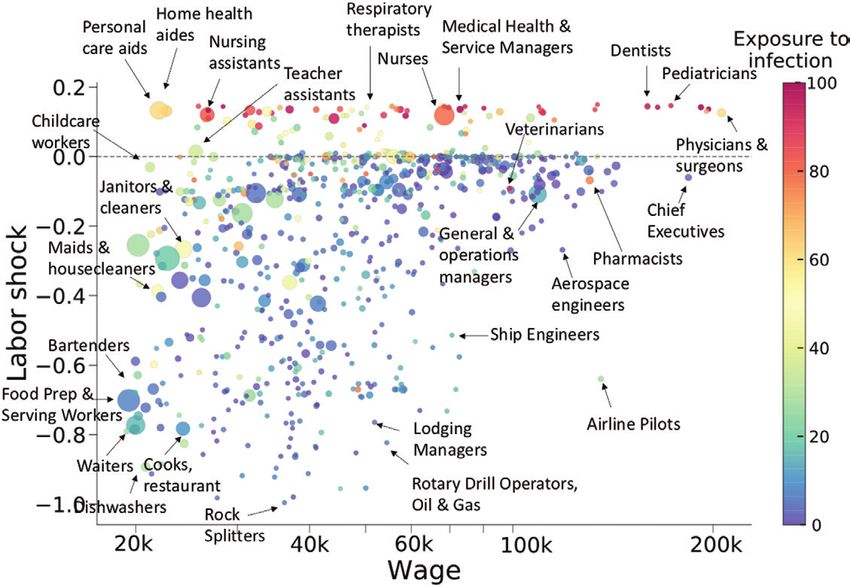
Supply and demand shocks in the COVID-19 pandemic                                                     S95

constrained by supply shocks. Entertainment, restaurants, and tourism face large supply and demand
shocks. At the occupation level, we show that high-wage occupations are relatively immune from ad-
verse supply- and demand-side shocks, while low-wage occupations are much more vulnerable. We
should emphasize that our results are only first-order shocks—we expect them to be substantially amp-
lified by feedback effects in the production network.

                                                                                                              Downloaded from https://academic.oup.com/oxrep/article/36/Supplement_1/S94/5899019 by guest on 02 October 2020
Keywords: COVID-19, shocks, economic growth, unemployment
JEL classification: I15, J21, J23, J63, O49

I.   Introduction
The COVID-19 pandemic is having an unprecedented impact on societies around the
world.1 As governments mandate social distancing practices and instruct non-essential
businesses to close to slow the spread of the outbreak, there is significant uncertainty
about the effect such measures will have on lives and livelihoods. While demand for
specific sectors such as grocery stores increased in the early weeks of the pandemic,
other sectors such as air transportation and tourism have seen demand for their services
evaporate. At the same time, many sectors are experiencing issues on the supply side, as
governments curtail the activities of non-essential industries and workers are confined
to their homes.
   In this paper, we aim to provide analytical clarity about the supply and demand
shocks caused by public health measures and changes in preferences caused by
avoidance of infection. We estimate (i) supply-side reductions due to the closure of
non-essential industries and workers not being able to perform their activities at home,
and (ii) demand-side changes due to peoples’ immediate response to the pandemic, such
as reduced demand for goods or services that are likely to place people at risk of infec-
tion (e.g. tourism).
   Several researchers have already provided estimates of the supply shock from labour
supply (Dingel and Neiman, 2020; Hicks et al., 2020; Koren and Petö, 2020). Here we
improve on these efforts in three ways: (i) we propose a methodology for estimating how
much work can be done from home, based on work activities, (ii) we identify industries
for which working from home is irrelevant because the industries are considered es-
sential, and (iii) we compare our estimated supply shocks to estimates of the demand
shock, which in many industries is the more relevant constraint on output.
   A number of papers have also emphasized the importance of demand-side factors
in the pandemic. For example, an early paper by Guerrieri et al. (2020) showed that,
in a two-sector new Keynesian model with low substitutability in consumption, asym-
metric labour supply shocks can lead to reductions in demand that are higher than the
initial shock. In their framework, sectoral heterogeneity is necessary for supply shocks
to lead to a larger demand impact. The scenario of a drop in demand larger than the
drop in supply is also plausible if long-term labour supply constraints lead to a col-
lapse of investment. This discussion underscores that supply and demand interact, and
supply shocks can lead to decreases in demand. But as we argue here, the COVID pan-
demic also created exogenous and instantaneous changes to consumer demand, both in

    1 This paper was prepared in March and early April 2020 and released on 16 April. This version contains

only minor changes rather than comprehensive updates.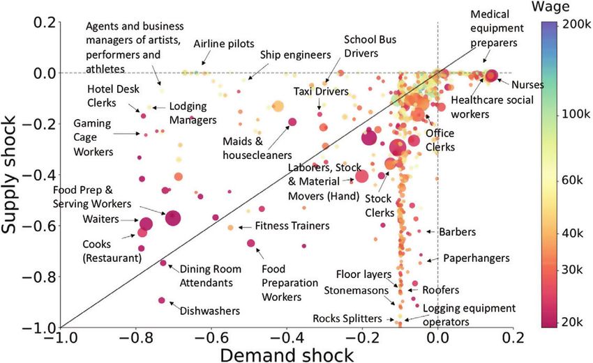
S96                                                                      R. Maria del Rio-Chanona et al.

magnitude and in composition as consumers’ preferences change in response to factors
such as infection risk, lower positive externalities in social consumption, explicit guide-
lines from the government, etc.
   To see why it is important to compare supply and demand shocks, consider the fol-
lowing thought experiment. Following social-distancing measures, suppose industry i is

                                                                                                                Downloaded from https://academic.oup.com/oxrep/article/36/Supplement_1/S94/5899019 by guest on 02 October 2020
capable of producing only 70 per cent of its pre-crisis output, e.g. because workers can
produce only 70 per cent of the output while working from home. If consumers reduce
their demand by 90 per cent, the industry will produce only what will be bought, that is,
10 per cent. If instead consumers reduce their demand by 20 per cent, the industry will
not be able to satisfy demand but will produce everything it can, that is, 70 per cent. In
other words, the experienced first-order reduction in output from the immediate shock
will be the greater of the supply and the demand shock.
   It is important to stress that the shocks that we predict here should not be interpreted
as the overall impact of the COVID-19 pandemic on the economy. Again, we expect
that as wages from work drop, there will be potentially larger second-order negative
impacts on demand, and the potential for a self-reinforcing downward spiral in output,
employment, income, and demand. Deriving overall impact estimates involves model-
ling second-order effects, such as the additional reductions in demand as workers who
are stood down or laid off experience a reduction in income, and additional reductions
in supply as potential shortages propagate through supply chains. Further effects, such
as cascading firm defaults, which can trigger bank failures and systemic risk in the fi-
nancial system, could also arise. Understanding these impacts requires a model of the
macro-economy and financial sector. In a companion paper (Pichler et al., 2020), we
present results from such an economic model, but we make our estimates of first-order
impacts available separately here, for other researchers or governments to build upon
or use in their own models.
   Overall, we find that the supply and demand shocks considered in this paper rep-
resent a reduction of around one-fifth of the US economy’s value added, one-quarter
of current employment, and about 16 per cent of the US total wage income.2 Supply
shocks account for the majority of this reduction. These effects vary substantially
across different industries. While we find no negative effects on value added for indus-
tries like Legal Services, Power Generation and Distribution, or Scientific Research,
the expected loss of value added reaches up to 80 per cent for Accommodation, Food
Services, and Independent Artists.
   We find that sectors such as Transport are likely to experience immediate demand-side
reductions that are larger than their corresponding supply-side shocks. Other industries
such as Manufacturing, Mining, and certain service sectors are likely to experience
larger immediate supply-side shocks relative to demand-side shocks. Entertainment,
restaurants, and hotels experience very large supply and demand shocks, with the de-
mand shock dominating. These results are important because supply and demand
shocks might have different degrees of persistence, and industries will react differently
to policies depending on the constraints that they face. Overall, however, we find that
aggregate effects are dominated by supply shocks, with a large part of manufacturing

    2 The results reported here are a slightly updated version of our work released on 16 April; we use a re-

vised and updated list of essential industries, and we no longer exclude owner-occupied dwellings (imputed
rents) from GDP (we assume no shocks to this sector). Our overall results do not change substantially.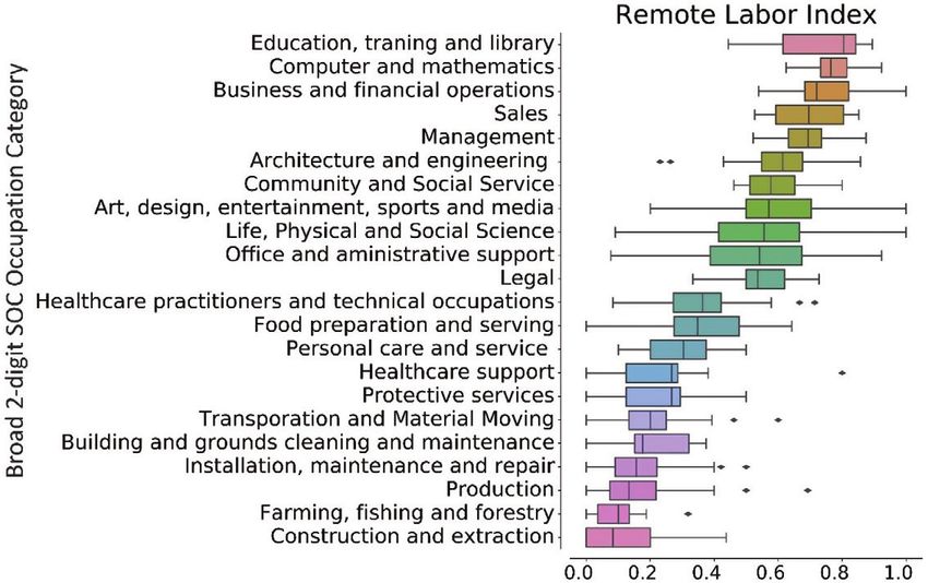
Supply and demand shocks in the COVID-19 pandemic                                                S97

and services being classified as non-essential while its labour force is unable to work
from home.
   We also break down our results by occupation and show that there is a strong nega-
tive relationship between the overall immediate shock experienced by an occupation
and its wage. Relative to the pre-COVID period, 41 per cent of the jobs for workers

                                                                                                       Downloaded from https://academic.oup.com/oxrep/article/36/Supplement_1/S94/5899019 by guest on 02 October 2020
in the bottom quartile of the wage distribution are predicted to be vulnerable. (And
bear in mind that this is only a first-order shock—second-order shocks may signifi-
cantly increase this.) In contrast, most high-wage occupations are relatively immune
from adverse shocks, with only 6 per cent of the jobs at risk for the 25 per cent of
workers working in the highest pay occupations. Absent strong support from govern-
ments, most of the economic burden of the pandemic will fall on lower wage workers.
   We neglect several effects that, while important, are small compared to those we con-
sider here. First, we have not sought to quantify the reduction in labour supply due to
workers contracting COVID-19. A rough estimate suggests that this effect is relatively
minor in comparison to the shocks associated with social-distancing measures that are
being taken in most developed countries.3 We have also not explicitly included the effect
of school closures. However, in Appendix D2. we argue that this is not the largest effect
and is already partially included in our estimates through indirect channels.
   A more serious problem is caused by the need to assume that within a given oc-
cupation, being unable to perform some work activities does not harm the perform-
ance of other work activities. Within an industry, we also assume that if workers in a
given occupation cannot work, they do not produce output, but this does not prevent
other workers in different occupations from producing. In both cases we assume that
the effects of labour on production are linear, i.e. that production is proportional to
the fraction of workers who can work. In reality, however, it is clear that there are
important complementarities leading to nonlinear effects. There are many situations
where production requires a combination of different occupations, such that if workers
in key occupations cannot work at home, production is not possible. For example, while
the accountants in a steel plant might be able to work from home, if the steelworkers
needed to run the plant cannot come to work, no steel is made. We cannot avoid making
linear assumptions because, as far as we know, there is no detailed understanding of
the labour production function and these interdependencies at an industry level. By
neglecting nonlinear effects, our work here should consequently be regarded as an ap-
proximate lower bound on the size of the first-order shocks.
   This paper focuses on the United States. We have chosen it as our initial test case be-
cause input–output tables are more disaggregated than those of most other countries,
and because the Occupational Information Network (O*NET) database, which we rely
on for information about occupations, was developed based on US data. With some
additional assumptions it is possible to apply the analysis we perform here to other de-
veloped countries.
   This paper is structured as follows. In section II we review the most relevant litera-
ture on the economic impact of the pandemic and the associated supply and demand
shocks. In section III we describe our methodology for estimating supply shocks,
which involves developing a new Remote Labour Index (RLI) for occupations and

            3   See Appendix D1. for rough quantitative estimates in support of this argument.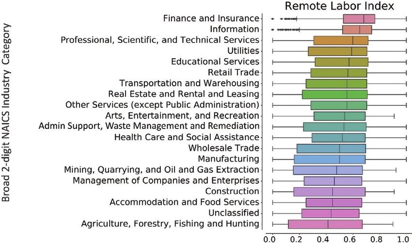
S98                                                                 R. Maria del Rio-Chanona et al.

combining it with a list of essential industries. Section IV discusses likely demand
shocks based on estimates developed by the US Congressional Budget Office (2006)
to predict the potential economic effects of an influenza pandemic. In section V, we
show a comparison of the supply and demand shocks across different industries and
occupations and identify the extent to which different activities are likely to be con-

                                                                                                      Downloaded from https://academic.oup.com/oxrep/article/36/Supplement_1/S94/5899019 by guest on 02 October 2020
strained by supply or demand. In this section, we also explore which occupations are
more exposed to infection and make comparisons to wage and occupation-specific
shocks. Finally, in section VI we discuss our findings in light of existing research and
outline avenues for future work. We also make all of our data available in a continu-
ously updated online repository (https://zenodo.org/record/3744959).

II.   Literature
Many economists and commentators believe that the economic impact could be dra-
matic (Baldwin and Weder di Mauro, 2020). To give an example based on survey data in
an economy under lockdown, the French statistical office estimated on 26 March 2020
that the economy is currently at around 65 per cent of its normal level.4 Bullard (2020)
provides an undocumented estimate that around a half of the US economy would be
considered either essential, or able to operate without creating risks of diffusing the
virus. Inoue and Todo (2020) modelled how shutting down firms in Tokyo would cause
a loss of output in other parts of the economy through supply chain linkages, and es-
timate that after a month, daily output would be 86 per cent lower than pre-shock (i.e.
the economy would be operating at only 14 per cent of its capacity!). Using a calibrated
extended consumption function, and assuming a labour income shock of 16 per cent
and various consumption shocks by expenditure categories, Muellbauer (2020) esti-
mates a fall of quarterly consumption of 20 per cent. Roughly speaking, most of these
estimates, like ours, are estimates of instantaneous declines, and would translate to
losses of annual GDP if the lockdown lasted for a year.
   Based on aggregating industry-level shocks, the OECD (2020) estimates a drop in
immediate GDP of around 25 per cent. Another study by Barrot et al. (2020) esti-
mates industry-level shocks by considering the list of essential industries, the closure of
schools, and an estimate of the ability to work from home (based on ICT use surveys).
Using these shocks in a multisector input–output model, they find that 6 weeks of so-
cial distancing would bring annual GDP down by 5.6 per cent.
   Our study predicts supply and demand shocks at a disaggregated level, and proposes
a simple method to calculate aggregate shocks from these. We take a short-term ap-
proach, and assume that the immediate drop in output is driven by the most binding
constraint—the worse of the supply and demand shock, essentially assuming that prices
do not adjust and markets do not clear. An alternative, standard in empirical macroeco-
nomics, is to observe aggregate changes in prices and quantities to infer the relative size
of the supply and demand shocks. For instance, Brinca et al. (2020) use data on wage
and hours worked; Balleer et al. (2020) use data on planned price changes in German
firms; and Bekaert et al. (2020) use surveys of inflation forecasts. While these studies do

                   4   https://www.insee.fr/en/statistiques/4473305?sommaire=4473307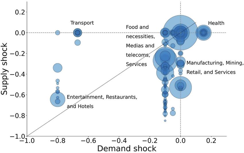
Supply and demand shocks in the COVID-19 pandemic                                                          S99

not agree on the relative importance of supply and demand shocks, an emerging con-
sensus is that both supply and demand shocks co-exist and are vastly different across
sectors, and over time.

                                                                                                                   Downloaded from https://academic.oup.com/oxrep/article/36/Supplement_1/S94/5899019 by guest on 02 October 2020
III.    Supply shocks
Supply shocks from pandemics are mostly thought of as labour supply shocks.
Several pre-COVID-19 studies focused on the direct loss of labour from death and
sickness (e.g. McKibbin and Sidorenko (2006), Santos et al. (2013)), although some
have also noted the potentially large impact of school closure (Keogh-Brown et al.,
2010). McKibbin and Fernando (2020) consider (among other shocks) reduced la-
bour supply due to mortality, morbidity due to infection, and morbidity due to the
need to care for affected family members. In countries where social distancing meas-
ures are in place, such measures will have a much larger economic effect than the
direct effects from mortality and morbidity. This is in part because if social distanc-
ing measures work, only a small share of population will be infected and die eventu-
ally. Appendix D1. provides more quantitative estimates of the direct mortality and
morbidity effects and argues that they are likely to be at least an order of magnitude
smaller than those due to social-distancing measures, especially if the pandemic is
contained.
   For convenience we neglect mortality and morbidity and assume that the supply
shocks are determined only by the amount of labour that is withdrawn due to social

Figure 1: A schematic network representation of supply-side shocks

Notes: The nodes to the left represent the list of essential industries at the NAICS 6-digit level. A green node
indicates essential, a red node non-essential. The orange nodes (centre-left) are more aggregate industry cat-
egories (e.g. 4-dig. NAICS or the BLS industry categories) for which further economic data are available. These
two sets of nodes are connected through industry concordance tables. The blue nodes (centre-right) are dif-
ferent occupations. A weighted link connecting an industry category with an occupation represents the number
of people of a given occupation employed in each industry. Nodes on the very right are O*NET work activities.
Green work activities mean that they can be performed from home, while red means that they cannot. O*NET
provides a mapping of work activities to occupations.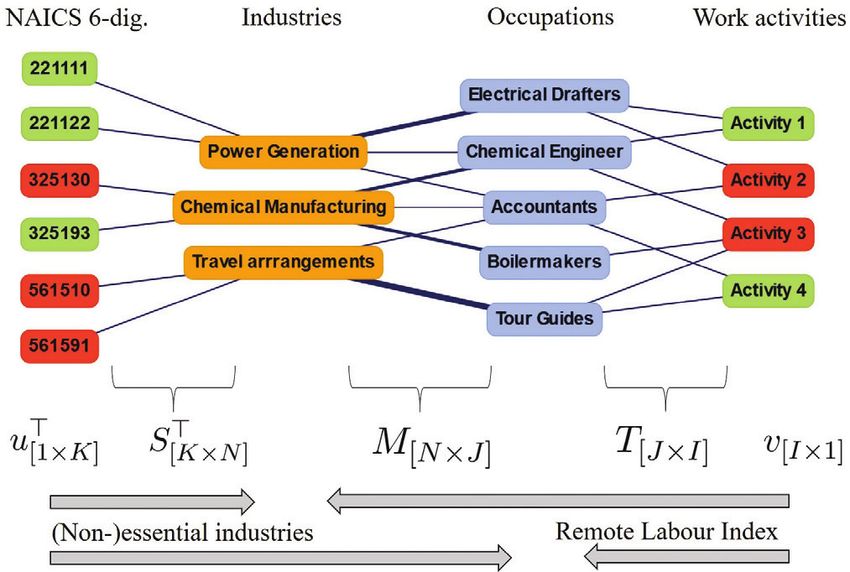
S100                                                                      R. Maria del Rio-Chanona et al.

distancing. We consider two key factors: (i) the extent to which workers in given oc-
cupations can perform their requisite activities at home, and (ii) the extent to which
workers are likely to be unable to come to work due to being in non-essential indus-
tries. We quantify these effects on both industries and occupations. Figure 1 gives a
schematic overview of how we predict industry and occupation specific supply shocks.

                                                                                                                  Downloaded from https://academic.oup.com/oxrep/article/36/Supplement_1/S94/5899019 by guest on 02 October 2020
We explain this in qualitative terms in the next few pages; for a formal mathematical
description see Appendix A.1.

(i)    How much work can be performed from home?
One way to assess the degree to which workers are able to work from home during the
COVID-19 pandemic is by direct survey. For example, Zhang et al. (2020) conducted
a survey of Chinese citizens in late February (1 month into the coronavirus-induced
lockdown in China) and found that 27 per cent of the labour force continued working
at the office, 38 per cent worked from home, and 25 per cent stopped working. Adams-
Prassl et al. (2020) surveyed US and UK citizens in late March, and reported that the
share of tasks that can be performed from home varies widely between occupations
(from around 20 to 70 per cent), and that higher wage occupations tend to be more able
to work from home.
   Other recent work has instead drawn on occupation-level data from O*NET to
determine labour shocks due to the COVID-19 pandemic. For example, Hicks et al.
(2020) drew on O*NET’s occupational Work Context Questionnaire and considered
the degree to which an occupation is required to ‘work with others’ or involves ‘physical
proximity to others’ in order to assess which occupations are likely to be most impacted
by social distancing. Dingel and Neiman (2020) aimed to quantify the number of jobs
that could be performed at home by analysing responses on O*NET’s Work Context
Questionnaire (such as whether the average respondent for an occupation spends the
majority of time walking or running or uses email less than once per month) as well
as responses on O*NET’s Generalized Work Activities Questionnaire (such as whether
performing general physical activities or handling and moving objects is very important
for a given occupation).
   In this study, we go to a more granular level than both the Work Context
Questionnaire and Generalized Work Activities Questionnaire, and instead draw on
O*NET’s ‘intermediate work activity’ data, which provide a list of the activities per-
formed by each occupation based on a list of 332 possible work activities. For example,
a nurse undertakes activities such as ‘maintain health or medical records’, ‘develop
patient or client care or treatment plans’, and ‘operate medical equipment’, while a
computer programmer performs activities such as ‘resolve computer programs’, ‘pro-
gram computer systems or production equipment’, and ‘document technical designs,
producers or activities’.5 In Figure 1 these work activities are illustrated by the right-
most set of nodes.

    5 In the future we intend to redo this using O*NET’s ‘detailed’ work activity data, which involve over

2,000 individual activities associated with different occupations. We believe this would somewhat improve our
analysis, but think that the intermediate activity list provides a good approximation. All updates will be made
available in the online data repository (see footnote 6).
Supply and demand shocks in the COVID-19 pandemic                                                     S101

Which work activities can be performed from home?
 Four of us independently assigned a subjective binary rating to each work activity as
to whether it could successfully be performed at home. The individual results were in
broad agreement. Based on the responses, we assigned an overall consensus rating to
each work activity.6 Ratings for each work activity are available in an online data reposi-

                                                                                                               Downloaded from https://academic.oup.com/oxrep/article/36/Supplement_1/S94/5899019 by guest on 02 October 2020
tory.7 While O*NET maps each intermediate work activity to 6-digit O*NET occupa-
tion codes, employment information from the US Bureau of Labor Statistics (BLS) is
available for the 4-digit 2010 Standard Occupation Scheme (SOC) codes, so we mapped
O*NET and SOC codes using a crosswalk available from O*NET.8 Our final sample
contains 740 occupations.

From work activities to occupations.
We then created a Remote Labour Index (RLI) for each occupation by calculating the
proportion of an occupation’s work activities that can be performed at home. An RLI
of 1 would indicate that all of the activities associated with an occupation could be
undertaken at home, while an RLI of 0 would indicate that none of the occupation’s
activities could be performed at home.9 The resulting ranking of each of the 740 occu-
pations can be found in the online repository (see footnote 6). In contrast to previous
work that has tended to arrive at binary assessments of whether an occupation can be
performed at home, our approach has the advantage of providing a unique indication
of the amount of work performed by a given occupation that can be done remotely.
While the results are not perfect,10 most of the rankings make sense. For example, in
Table 1, we show the top 20 occupations having the highest RLI ranking. Some occu-
pations such as credit analysts, tax preparers, and mathematical technician occupations
are estimated to be able to perform 100 per cent of their work activities from home.
Table 1 also shows a sample of the 43 occupations with an RLI ranking of zero, i.e.
those for which there are no activities that can be performed at home.
   To provide a broader perspective of how the RLI differs across occupation categories,
Figure 2 shows a series of box-plots indicating the distribution of RLI for each 4-digit
occupation in each 2-digit SOC occupation category. We have ordered 2-digit SOC oc-
cupations in accordance with their median values. Occupations with the highest RLI
relate to Education, Training and Library, Computer and Mathematical, and Business
and Financial roles, while occupations relating to Production, Farming, Fishing and
Forestry, and Construction and Extraction tend to have lower RLI.
     6 An activity was considered to be able to be performed at home if three or more respondents rated this

as true. We also undertook a robustness analysis where an activity was considered to be able to be performed
at home based on two or more true ratings. Results remained fairly similar. In post-survey discussion, we
agreed that the most contentious point is that some work activities might be done from home or not, de-
pending on the industry in which they are performed.
     7 https://zenodo.org/record/3744959
     8 Available at https://www.onetcenter.org/crosswalks.html
     9 We omitted ten occupations that had fewer than five work activities associated with them. These occu-

pations include Insurance Appraisers Auto Damage; Animal Scientists; Court Reporters; Title Examiners,
Abstractors, and Searchers; Athletes and Sports Competitors; Shampooers; Models; Fabric Menders, Except
Garment; Slaughterers and Meat Packers; and Dredge Operators.
     10 There are a few cases that we believe are misclassified. For example, two occupations with a high

RLI that we think cannot be performed remotely are real estate agents (RLI = 0.7) and retail salespersons
(RLI = 0.63). However, these are exceptions—in most cases the rankings make sense.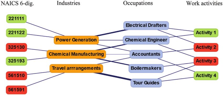
S102                                                                    R. Maria del Rio-Chanona et al.

Table 1: Top and bottom 20 occupations ranked by Remote Labour Index (RLI), based on proportion of
work activities that can be performed at home

Occupation                                                                                            RLI

Credit Analysts                                                                                      1.00

                                                                                                             Downloaded from https://academic.oup.com/oxrep/article/36/Supplement_1/S94/5899019 by guest on 02 October 2020
Insurance Underwriters                                                                               1.00
Tax Preparers                                                                                        1.00
Mathematical Technicians                                                                             1.00
Political Scientists                                                                                 1.00
Broadcast News Analysts                                                                              1.00
Operations Research Analysts                                                                         0.92
Eligibility Interviewers, Government Programs                                                        0.92
Social Scientists and Related Workers, All Other                                                     0.92
Technical Writers                                                                                    0.91
Market Research Analysts and Marketing Specialists                                                   0.90
Editors                                                                                              0.90
Business Teachers, Postsecondary                                                                     0.89
Management Analysts                                                                                  0.89
Marketing Managers                                                                                   0.88
Mathematicians                                                                                       0.88
Astronomers                                                                                          0.88
Interpreters and Translators                                                                         0.88
Mechanical Drafters                                                                                  0.86
Forestry and Conservation Science Teachers, Postsecondary                                            0.86
...                                                                                                   ...
Bus and Truck Mechanics and Diesel Engine Specialists                                                0.00
Rail Car Repairers                                                                                   0.00
Refractory Materials Repairers, Except Brickmasons                                                   0.00
Musical Instrument Repairers and Tuners                                                              0.00
Wind Turbine Service Technicians                                                                     0.00
Locksmiths and Safe Repairers                                                                        0.00
Signal and Track Switch Repairers                                                                    0.00
Meat, Poultry, and Fish Cutters and Trimmers                                                         0.00
Pourers and Casters, Metal                                                                           0.00
Foundry Mold and Coremakers                                                                          0.00
Extruding and Forming Machine Setters,                                                               0.00
Operators, and Tenders, Synthetic and Glass Fibers
Packaging and Filling Machine Operators and Tenders                                                  0.00
Cleaning, Washing, and Metal Pickling Equipment Operators and Tenders                                0.00
Cooling and Freezing Equipment Operators and Tenders                                                 0.00
Paper Goods Machine Setters, Operators, and Tenders                                                  0.00
Tire Builders                                                                                        0.00
Helpers–Production Workers                                                                           0.00
Production Workers, All Other                                                                        0.00
Machine Feeders and Offbearers                                                                       0.00
Packers and Packagers, Hand                                                                          0.00

Note: There are 44 occupations with an RLI of zero; we show only a random sample.

From occupations to industries.
 We next map the RLI to industry categories to quantify industry-specific supply shocks
from social distancing measures. We obtain occupational compositions per industry
from the BLS, which allows us to match 740 occupations to 277 industries.11
    11 We use the May 2018 Occupational Employment Statistics (OES) estimates on the level of 4-digit
NAICS (North American Industry Classification System), file nat4d_M2018_dl, which is available at https://
www.bls.gov/oes/tables.htm under All Data. Our merged dataset covers 136.8 out of 144 million employed
people (95 per cent) initially reported in the OES.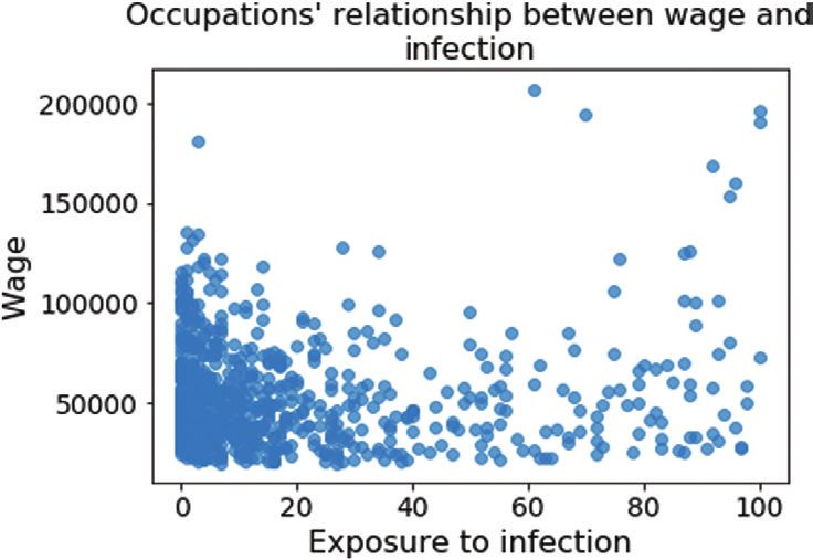
Supply and demand shocks in the COVID-19 pandemic                                                        S103

Figure 2: Distribution of RLI across occupations

                                                                                                                   Downloaded from https://academic.oup.com/oxrep/article/36/Supplement_1/S94/5899019 by guest on 02 October 2020
Note: We provide boxplots showing distribution of RLI for each 4-digit occupation in each 2-digit SOC occupa-
tion category.

Figure 3: Distribution of RLI across industries

Note: We provide boxplots showing distribution of RLI for each 4-digit occupation in each 2-digit NAICS Industry
category.
S104 R. Maria del Rio-Chanona et al.
In Figure 3, we show the RLI distribution for each 4-digit occupation category
falling within each broad 2-digit NAICS category. Similar to Figure 2, we have ordered
the 2-digit NAICS industry categories in accordance with the median values of each
underpinning distribution. As there is a greater variety of different types of occupations
within these broader industry categories, distributions tend to be much wider. Industries
Downloaded from https://academic.oup.com/oxrep/article/36/Supplement_1/S94/5899019 by guest on 02 October 2020
with the highest median RLI values relate to Information, Finance and Insurance, and
Professional, Science and Technical Services, while industries with the lowest median
RLI relate to Agriculture, Forestry, Fishing and Hunting and Accommodation and
Food Services.
In Appendix B, we show industry-specific RLI values for the more detailed 4-digit
NAICS industries. To arrive at a single number for each 4-digit industry, we compute
the employment-weighted average of occupation-specific RLIs. The resulting industry-
specific RLI can be interpreted as a rough estimate of the fraction of jobs which can be
performed from home for each industry.
(ii) Which industries are ‘essential’?
Across the world, many governments have mandated that certain industries deemed
‘essential’ should remain open over the COVID-19 crisis duration. What constitutes an
‘essential’ industry has been the subject of significant debate, and it is likely that the en-
dorsed set of essential industries will vary across countries. As the US government has
not produced a definitive list, here we draw on the list of essential industries developed
by Italy and assume it can be applied, at least as an approximation, to other countries,
such as the US, as well. This list has two key advantages. First, as Italy was one of
the countries affected earliest and most severely, it was one of the first countries to in-
vest significant effort considering which industries should be deemed essential. Second,
Italy’s list of essential industries includes NACE industrial classification codes, which
can be mapped to the NAICS industry classification we use to classify industrial em-
ployment in this paper.12
Table 2: Essential industries
Total 6-digit NAICS industries 1,057
Number of essential 6-digit NAICS industries 612
Fraction of essential industries at 6-digit NAICS 0.58
Total 4-digit NAICS industries in our sample 277
Average rating of essential industries at 4-digit NAICS 0.56
Fraction of labour force in essential industries 0.67
Notes: Essential industries at the 6-digit level and essential ‘share’ at the 4-digit level. Note that 6-digit NAICS
industry classifications are binary (0 or 1) whereas 4-digit NAICS industry classifications can take on any value
between 0 and 1.
12 Mapping NACE industries to NAICS industries is not straightforward. NACE industry codes at the
4-digit level are internationally defined. However, 6-digit level NACE codes are country specific. Moreover,
the list of essential industries developed by Italy involves industries defined by varying levels of aggregation.
Most essential industries are defined at the NACE 2-digit and 4-digit level, with a few 6-digit categories
thrown in for good measure. As such, much of our industrial mapping methodology involved mapping from
one classification to the other by hand. We provide a detailed description of this process in Appendix B.1.Supply and demand shocks in the COVID-19 pandemic S105
Table 2 shows the total numbers of NAICS essential industries at the 6-digit and
4-digit level. More than 50 per cent of 6-digit NAICS industries are considered essential.
At the 6-digit level the industries are either classified as essential, and assigned essential
score 1, or non-essential and assigned essential score 0. Unfortunately, it is not possible
to translate this directly into a labour force proportion as BLS employment data at de-
Downloaded from https://academic.oup.com/oxrep/article/36/Supplement_1/S94/5899019 by guest on 02 October 2020
tailed occupation and industry levels are only available at the NAICS 4-digit level. To
derive an estimate at the 4-digit level, we assume that labour in a NAICS 4-digit code is
uniformly distributed over its associated 6-digit codes. We then assign an essential ‘share’
to each 4-digit NAICS industry based on the proportion of its 6-digit NAICS industries
that are considered essential. (The distribution of the essential share over 4-digit NAICS
industries is shown in Appendix B.) Based on this analysis, we estimate that about 92m
(or 67 per cent) of US workers are currently employed in essential industries.
(iii) Supply shock: non-essential industries unable to work
from home
Having analysed both the extent to which jobs in each industry are essential and the
likelihood that workers in a given occupation can perform their requisite activities at
home, we now combine these to consider the overall first-order effect on labour supply
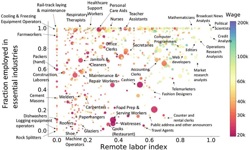
in the US. In Figure 4, we plot the RLI of each occupation against the fraction of that
occupation employed in an essential industry. Each circle in the scatter plot represents
an occupation; the circles are sized proportional to current employment and colour
coded according to the median wage in each occupation.
Figure 4: Fraction employed in an essential industry vs Remote Labour Index for each occupation
Notes: Omitting the effect of demand reduction, the occupations in the lower left corner, with a small proportion
of workers in essential industries and a low Remote Labour Index, are the most vulnerable to loss of employ-
ment due to social distancing.S106 R. Maria del Rio-Chanona et al.
Figure 5: Workers that cannot work
Downloaded from https://academic.oup.com/oxrep/article/36/Supplement_1/S94/5899019 by guest on 02 October 2020
Notes: On the left is the percentage of workers in a non-essential job (33 per cent in total). On the right is the
percentage of workers that cannot work remotely (56 per cent in total). The intersection is the set of workers
that cannot work, which is 19 per cent of all workers. A remaining 30 per cent of workers are in essential jobs
where they can work remotely.
Figure 4 indicates the vulnerability of occupations due to supply-side shocks.
Occupations in the lower left-hand side of the plot (such as Dishwashers, Rock Splitters,
and Logging Equipment Operators) have lower RLI scores (indicating they are less able
to work from home) and are less likely to be employed in an essential industry. If we
consider only the immediate supply-side effects of social distancing, workers in these
occupations are more likely to face reduced work hours or be at risk of losing their jobs
altogether. In contrast, occupations on the upper right-hand side of the plot (such as
Credit Analysis, Political Scientists, and Operations Research Analysts) have higher
RLI scores and are more likely to be employed in an essential industry. These occupa-
tions are less economically vulnerable to the supply-side shocks (though, as we discuss
in the next section, they could still face employment risks due to first-order demand-
side effects). Occupations in the upper-left hand side of the plot (such as Farmworkers,
Healthcare Support Workers, and Respiratory Therapists) are less likely to be able to
perform their job at home, but since they are more likely to be employed in an essential
industry their economic vulnerability from supply-side shocks is lower. Interestingly,
there are relatively few occupations on the lower-right hand side of the plot. This in-
dicates that occupations that are predominantly employed in non-essential industries
tend to be less able to perform their activities at home.
To help visualize the aggregate numbers we provide a summary in the form of a Venn
diagram in Figure 5. Before the pandemic, 33 per cent of workers were employed in
non-essential jobs. 56 per cent of workers are estimated to be unable to perform their job
remotely. 19 per cent of workers are in the intersection corresponding to non-essential
jobs that cannot be performed remotely. In addition, there are 30 per cent of workers in
essential industries that can also work from home.13
13 In fact we allow for a continuum between the ability to work from home, and an industry can be par-
tially essential.Supply and demand shocks in the COVID-19 pandemic S107
IV. Demand shock
The pre-COVID-19 literature on epidemics and the discussions of the current crisis
make it clear that epidemics strongly influence patterns of consumer spending.
Consumers are likely to seek to reduce their risk of exposure to the virus and decrease
Downloaded from https://academic.oup.com/oxrep/article/36/Supplement_1/S94/5899019 by guest on 02 October 2020
demand for products and services that involve close contact with others. In the early
days of the outbreak, stockpiling behaviour also drives a direct demand increase in the
retail sector (Baker et al., 2020).
Estimates from the CBO
Our estimates of the demand shock are based on expert estimates developed by the
US Congressional Budget Office (2006) that attempted to predict the potential impact
of an influenza pandemic. Similar to the current COVID-19 pandemic, this analysis
assumes that demand is reduced due to the desire to avoid infection. While the analysis
is highly relevant to the present COVID-19 situation, it is important to note that the
estimates are ‘extremely rough’ and ‘based loosely on Hong Kong’s experience with
SARS’. The CBO provides estimates for two scenarios (mild and severe). We draw on
the severe scenario, which
describes a pandemic that is similar to the 1918–1919 Spanish flu outbreak. It
incorporates the assumption that a particularly virulent strain of influenza in-
fects roughly 90 million people in the United States and kills more than 2 million
of them.
In this paper, we simply take the CBO estimates as immediate (first-order) demand-side
shocks. The CBO lists demand-side estimates for broad industry categories, which we
mapped to the 2-digit NAICS codes by hand. Table 3 shows the CBO’s estimates of
the percent decrease in demand by industry, and Table 8 in Appendix E shows the full
mapping to 2-digit NAICS.
These estimates, of course, are far from perfect. They are based on expert estimates
made more than 10 years ago for a hypothetical pandemic scenario. It is not entirely clear
if they are for gross output or for final (consumer) demand. However, in Appendix E,
we describe three other sources of consumption shocks (Keogh-Brown et al., 2010;
Muellbauer, 2020; OECD, 2020) that provide broadly similar estimates by industry or
spending category. We also review papers that have appeared more recently and con-
tained estimates of consumption changes based on transaction data. Taken together,
these papers suggest that the shocks from the CBO were qualitatively accurate: very
large declines in the hospitality, entertainment, and transport industries, milder declines
in manufacturing, and a more resistant business services sector. The main features that
have been missed are the increase in demand, at least early on, in some specific retail
categories (groceries), and the decline in health consumption, in sharp contrast with the
CBO prediction of a 15 per cent increase.
Aggregate consumption vs composition of the shocks
The shocks from the CBO include two separate effects: a shift of preferences, where the
utility of healthcare relative to restaurants, say, increases; and an aggregate consump-
tion effect. Here, we do not go further in distinguishing these effects, although thisS108 R. Maria del Rio-Chanona et al.
Table 3: Demand shock by sector according to the Congressional Budget Office (2006)’s severe
scenario
Broad industry name Severe scenario shock
Agriculture –10
Downloaded from https://academic.oup.com/oxrep/article/36/Supplement_1/S94/5899019 by guest on 02 October 2020
Mining –10
Utilities 0
Construction –10
Manufacturing –10
Wholesale trade –10
Retail trade –10
Transportation and warehousing –67
(including air, rail, and transit)
Information (published, broadcast) 0
Finance 0
Professional and business services 0
Education 0
Healthcare 15
Arts and recreation –80
Accommodation/food service –80
Other services except government –5
Government 0
becomes necessary in a more fully-fledged model (Pichler et al., 2020). Yet, it remains
instructive to note that, in Muellbauer’s (2020) consumption function estimates, the de-
cline in aggregate consumption is not only due to direct changes in consumption in spe-
cific sectors, but also to lower income, rising income insecurity (due to unemployment
in particular), and wealth effects (due in particular to falling asset prices).
Transitory and permanent shocks
An important question is whether demand reductions are just postponed expenses, and
if they are permanent (Keogh-Brown et al., 2010; Mann, 2020). Baldwin and Weder di
Mauro (2020) also distinguish between ‘practical’ (the impossibility to shop) and ‘psy-
chological’ (the wait-and-see attitude adopted by consumers facing strong uncertainty)
demand shocks. We see three possibilities: (i) expenses in a specific good or service
are just delayed but will take place later, for instance if households do not go to the
restaurant this quarter, but go twice as often as they would normally during the next
quarter; (ii) expenses are not incurred this quarter, but will come back to their normal
level after the crisis, meaning that restaurants will have a one-quarter loss of sales; and
(iii) expenses decrease to a permanently lower level, as household change their pref-
erences in view of the ‘new normal’. Appendix E reproduces the scenario adopted by
Keogh-Brown et al. (2010), which distinguishes between delay and permanently lost
expenses.
Other components of aggregate demand
We do not include direct shocks to investment, net exports, and net inventories.
Investment is typically very pro-cyclical and is likely to be strongly affected, with direct
factors including cash-flow reductions and high uncertainty (Boone, 2020). The im-
pact on trade is likely to be strong and possibly permanent (Baldwin and Weder di
Mauro, 2020), but would affect exports and imports in a relatively similar way, so theSupply and demand shocks in the COVID-19 pandemic S109
overall effect on net exports is unclear. Finally, it is likely that due to the disruption of
supply chains, inventories will be run down so the change in inventories will be negative
(Boone, 2020).
Downloaded from https://academic.oup.com/oxrep/article/36/Supplement_1/S94/5899019 by guest on 02 October 2020
V. Combining supply and demand shocks
Having described both supply- and demand-side shocks, we now compare the two at
the industry and occupation level.
(i) Industry-level supply and demand shocks
Figure 6 plots the demand shock against the supply shock for each industry. The ra-
dius of the circles is proportional to the gross output of the industry.14 Essential in-
dustries have no supply shock and so lie on the horizontal ‘0’ line. Of these industries,
sectors such as Utilities and Government experience no demand shock either, since
immediate demand for their output is assumed to remain the same. Following the
CBO predictions, Health experiences an increase in demand and consequently lies
Figure 6: Supply and demand shocks for industries
Notes: Each circle is an industry, with radius proportional to gross output. Many industries experience exactly
the same shock, hence the superposition of some of the circles. Labels correspond to broad classifications of
industries.
14 Since relevant economic variables such as total output per industry are not extensively available on
the NAICS 4-digit level, we need to further aggregate the data. We derive industry-specific total output and
value added for the year 2018 from the BLS input–output accounts, allowing us to distinguish 170 industries
for which we can also match the relevant occupation data. The data can be downloaded from https://www.
bls.gov/emp/data/input-output-matrix.htm.S110 R. Maria del Rio-Chanona et al.
Figure 7: Supply and demand shocks for occupations
Downloaded from https://academic.oup.com/oxrep/article/36/Supplement_1/S94/5899019 by guest on 02 October 2020
Notes: Each circle is an occupation with radius proportional to employment. Circles are colour coded by the
log median wage of the occupation. The correlation between median wages and demand shocks is 0.26
(p-value = 2.8 × 10⁻¹³) and between median wages and supply shocks is 0.41 (p-value = 1.5 × 10⁻³⁰).
below the identity line. Transport, on the other hand, experiences a reduction in de-
mand and lies well above the identity line. This reflects the current situation, where
trains and buses are running because they are deemed essential, but they are mostly
empty. Non-essential industries such as Entertainment, Restaurants, and Hotels, ex-
perience both a demand reduction (due to consumers seeking to avoid infection) and
a supply reduction (as many workers are unable to perform their activities at home).
Since the demand shock is bigger than the supply shock, they lie above the identity
line. Other non-essential industries, such as Manufacturing, Mining, and Retail, have
supply shocks that are larger than their demand shocks and consequently lie below the
identity line.
(ii) Occupation-level supply and demand shocks
In Figure 7 we show the supply and demand shocks for occupations rather than in-
dustries. For each occupation this comparison indicates whether it faces a risk of un-
employment due the lack of demand or a lack of supply in its industry.
Several health-related occupations, such as Nurses, Medical Equipment Preparers,
and Healthcare Social Workers, are employed in industries experiencing increased de-
mand. Occupations such as Airline Pilots, Lodging Managers, and Hotel Desk Clerks
face relatively mild supply shocks and strong demand shocks (as consumers reduce
their demand for travel and hotel accommodation) and consequently lie above the
identity line. Other occupations such as Stonemasons, Rock Splitters, Roofers, andSupply and demand shocks in the COVID-19 pandemic S111
Floor Layers face a much stronger supply shock as it is very difficult for these workers
to perform their job at home. Finally, occupations such as Cooks, Dishwashers, and
Waiters suffer both adverse demand shocks (since demand for restaurants is reduced)
and supply shocks (since they cannot work from home and tend not to work in essen-
tial industries).
Downloaded from https://academic.oup.com/oxrep/article/36/Supplement_1/S94/5899019 by guest on 02 October 2020
For the majority of occupations, the supply shock is larger than the demand shock.
This is not surprising given that we only consider immediate shocks and no feedback-
loops in the economy. We expect that once second-order effects are considered the de-
mand shocks are likely to be much larger.
(iii) Aggregate shocks
We now aggregate shocks to obtain estimates for the whole economy. We as-
sume that, in a given industry, the total shock will be the largest of the supply
or demand shocks. For example, if an industry faces a 30 per cent demand
shock and 50 per cent supply shock because 50 per cent of the industry’s work-
force cannot work, the industry is assumed to experience an overall 50 per cent
shock to output. For simplicity, we assume a linear relationship between output
and labour: i.e. when industries are supply constrained, output is reduced by the
same fraction as the reduction in labour supply. This assumption also implies
that the demand shock that workers of an industry experience equals the indus-
try’s output demand shock in percentage terms. For example, if transport faces
a 67 per cent demand shock and no supply shock, bus drivers working in this in-
dustry will experience an overall 67 per cent employment shock. The shock on
occupations depends on the prevalence of each occupation in each industry (see
Appendix A for details). We then aggregate shocks in three different ways.
First, we estimate the decline in employment by weighting occupation-level shocks
by the number of workers in each occupation. Second, we estimate the decline in total
wages paid by weighting occupation-level shocks by the share of occupations in the
total wage bill. Finally, we estimate the decline in GDP by weighting industry-level
shocks by the share of industries in GDP.15
Table 4: Aggregate shocks to employment, wages, and value added
Aggregate shock Employment Wages Value added
Supply –19 –14 –16
Demand –13 –8 –7
Total –23 –16 –20
Notes: The size of each shock is shown as a percentage of the pre-pandemic value. Demand shocks include
positive values for the health sector. The total shock at the industry level is the minimum of the supply and de-
mand shock, see Appendix A. Note that these are only first-order shocks (not total impact), and instantaneous
values (not annualized).
15 Since rents account for an important part of GDP, we make an additional robustness check by consid-
ering the Real Estate sector essential. In this scenario the supply and total shocks drop by 3 percentage points.S112 R. Maria del Rio-Chanona et al.
Table 4 shows the results. In all cases, by definition, the total shock is larger than both
the supply and demand shock, but smaller than the sum. Overall, the supply shock ap-
pears to contribute more to the total shock than does the demand shock.
The wage shock is around 16 per cent and is lower than the employment shock
(23 per cent). This makes sense, and reflects a fact already well acknowledged
Downloaded from https://academic.oup.com/oxrep/article/36/Supplement_1/S94/5899019 by guest on 02 October 2020
in the literature (Office for National Statistics, 2020; Adams-Prassl et al., 2020)
that occupations that are most affected tend to have lower wages. We discuss this
more below.
For industries and occupations in the health sector, which experience an increase
in demand in our predictions, there is no corresponding increase in supply. Table 6 in
Appendix A.7 provides the same estimates as Table 4, but now assuming that the in-
creased demand for health will be matched by increased supply. This corresponds to a
scenario where the healthcare sector would be immediately able to hire as many workers
as necessary and pay them at the normal rate. This assumption does not, however, make
a significant difference to the aggregate total shock. In other words, the increase in ac-
tivity in the health sector is unlikely to be large enough to compensate significantly for
the losses from other sectors.
(iv) Shocks by wage level
To understand how the pandemic has affected workers of different income levels differ-
ently, we present results for each wage quartile. The results are in Table 5, columns q1 ...
q4,16 where we show employment shocks by wage quartile. This table shows that workers
whose wages are in the lowest quartile (lowest 25 per cent) will bear much higher rela-
tive losses than workers whose wages are in the highest quartile. Our results confirm the
survey evidence reported by the Office for National Statistics (2020) and Adams-Prassl
et al. (2020), showing that low-wage workers are more strongly affected by the COVID
crisis in terms of lost employment and lost income. Furthermore, Table 5 shows how
the total loss of wages in the economy is split amongst the different quartiles. Even
though those in the lowest quartile have lower salary, the shock is so high that they bear
the highest share of the total loss.
Next we estimate labour shocks at the occupation level. We define the labour shocks
as the declines in employment due to the total shocks in the industries associated with
Table 5: Total wages or employment shocks by wage quartile
q1 q2 q3 q4 Aggregate
Percentage change in employment –41 –23 –20 –6 –23
Share of total lost wages (%) 31 24 29 17 –16
Notes: We divide workers into wage quartiles based on the average wage of their occupation (q1 corresponds
to the 25 per cent least-paid workers). The first row is the number of workers who are vulnerable due to the
shock in each quartile divided by the total who are vulnerable. Similarly, the second row is the fraction of whole
economy total wages loss that would be lost by vulnerable workers in each quartile. The last column gives the
aggregate shocks from Table 4.
16 As before, Table 6 in Appendix A.7 gives the results assuming positive total shocks for the health
sector, but shows that it makes very little difference.Supply and demand shocks in the COVID-19 pandemic S113
Figure 8: Labour shock vs median wage for different occupations
Downloaded from https://academic.oup.com/oxrep/article/36/Supplement_1/S94/5899019 by guest on 02 October 2020
Notes: We colour occupations by their exposure to disease and infection. There is a 0.40 correlation between
wages and the labour shock (p-value = 3.5 × 10⁻³⁰). Note the striking lack of high-wage occupations with large
labour demand shocks.
each occupation. We use Eq. (14) (Appendix A.7) to compute the labour shocks, which
allows for positive shocks in healthcare workers, to suggest an interpretation in terms
of a change in labour demand. Figure 8 plots the relationship between labour shocks
and median wage. A strong positive correlation (Pearson ρ = 0.40, p-value = 3.5 ×
10–30) is clearly evident, with almost no high-wage occupations facing a serious shock.
We have also coloured occupations by their exposure to disease and infection using
an index developed by O*NET17 (for brevity we refer to this index as ‘exposure to in-
fection’). As most occupations facing a positive labour shock relate to healthcare,18 it
is not surprising to see that they have a much higher risk of being exposed to disease
and infection. However, other occupations such as janitors, cleaners, maids, and child-
care workers also face higher risk of infection. Appendix C explores the relationship
between exposure to infection and wage in more detail.
VI. Conclusion
This paper has sought to provide quantitative predictions for the US economy of the
supply and demand shocks associated with the COVID-19 pandemic. To characterize
17 https://www.onetonline.org/find/descriptor/result/4.C.2.c.1.b
18 Our demand shocks do not have an increase in retail but, in the UK, supermarkets have been trying
to hire several tens of thousands of workers (Source: BBC, 21 March, https://www.bbc.co.uk/news/busi-
ness-51976075). Baker et al. (2020) document stock-piling behaviour in the US.You can also read