GLOBAL ECONOMY MUNICH, 13-14 MAY 2021 CITIES AND THE SEA LEVEL - YATANG LIN, THOMAS K.J. MCDERMOTT, AND GUY MICHAELS - CESIFO
←
→
Page content transcription
If your browser does not render page correctly, please read the page content below
Global Economy
Munich, 13–14 May 2021

Cities and the Sea Level
Yatang Lin, Thomas K.J. McDermott, and Guy Michaels
Cities and the Sea Level
               Yatang Lin (Hong Kong University of Science and Technology)
           Thomas K.J. McDermott (National University of Ireland Galway and LSE)
                        Guy Michaels (London School of Economics)

                                                  April 1, 2021

                                                     Abstract

          Construction on low elevation coastal zones is risky for both residents and taxpayers who bail
      them out, especially when sea levels are rising. We study this construction using spatially disag-
      gregated data on the US Atlantic and Gulf coasts. We document nine stylized facts, including a
      sizeable rise in the share of coastal housing built on flood-prone land from 1990-2010, which con-
      centrated particularly in densely populated areas. To explain our findings, we develop a model
      of a monocentric coastal city, which we then use to explore the consequences of sea level rise and
      government policies.

    KEYWORDS: Cities, Climate Change, Sea Level Rise.

    JEL CLASSIFICATION: R11, Q54, R14

1    Introduction
Where do people build houses in low elevation coastal zones (LECZ)? Some construction in LECZ
puts residents at risk and exposes taxpayers who pay for bailouts, problems which sea level rise
(SLR) exacerbates. We study the location of existing and new housing on LECZ in the US, using SLR
maps and census data at a fine spatial scale. Using these data, we document nine stylized facts. One
of our findings is that within 10km of the Atlantic and Gulf coasts, 12 percent of the 1990 housing
stock was in flood-prone areas, but this share increased to 26 percent for net new construction from
1990-2010. We also show that this new construction in flood-prone areas concentrated particularly in
densely populated areas. To understand why this happened, we develop a model of a monocentric
coastal city, which explains our stylized facts. We then extend the model to explore the potential
consequences of SLR in LECZ.
     Corresponding author: Michaels (g.michaels@lse.ac.uk). We thank Juan Alvarez-Vilanova and Tiernan Evans for ex-
cellent research assistance. We thank Emek Basker, Vernon Henderson, Alan Manning, Henry Overman, Steve Pischke,
Eric Strobl, and John Van Reenen, and seminar/conference participants at Bank of Spain, ERSA 2018, IFAU, LSE, NUI
Galway, University of Kent, University of Stockholm, UPF, and the US Census Bureau for their helpful comments. We are
grateful to the Hong Kong University Grant Committee, Irish Research Council award no. GOIPD/2017/1147, and the
ESRC’s Centre for Economic Performance for their generous financial support.

                                                            1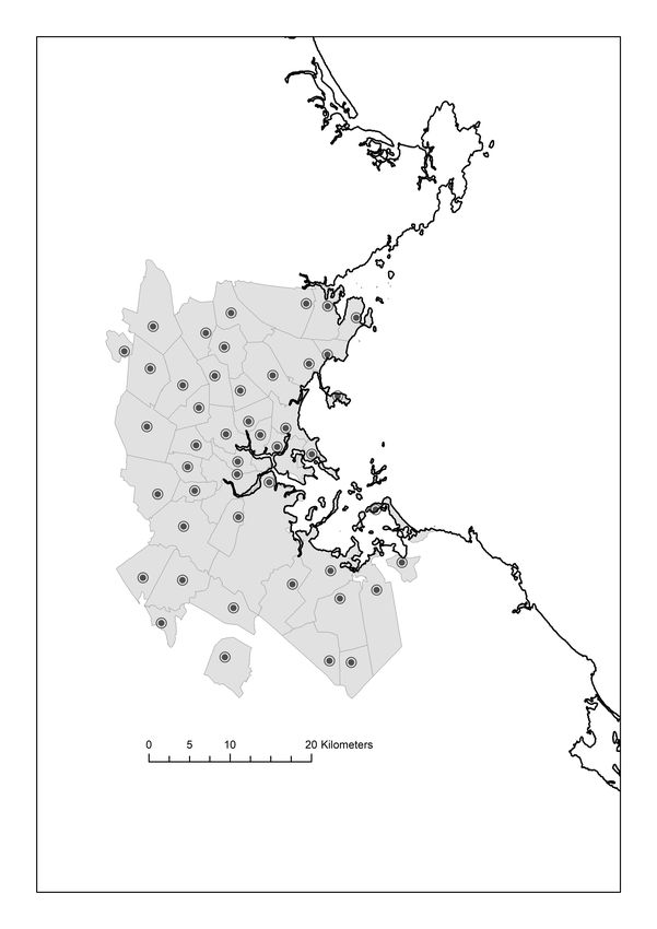
LECZ are often attractive places to live. Neumann et al. (2015) estimate that in 2000 they were
home to around 10.2% of the world’s population (625 million people), a figure expected to grow
significantly by 2050.1 But this growing attraction of LECZ poses problems, due to their susceptibil-
ity to floods. Over the past 36 years, floods worldwide killed more than 680 thousand people and
displaced more than 650 million (Brakenridge 2021). And the conditions in LECZ are expected to
worsen, as climate change warms the world’s oceans and melts some of its glaciers. The UN’s Inter-
governmental Panel on Climate Change, IPCC (Pörtner et al. 2019), forecasts that mean global sea
levels will rise by 43-84 centimeters by 2100. To compound the problem, climate change may also
increase the severity of tropical storms (Berardelli 2019). All this is expected to rapidly raise global
annual flood costs, which may exceed $1 trillion by 2050 (Hallegatte et al. 2013).
    The problem of flooding – ranging from nuisance flooding to extreme flooding by tropical storms
– is acutely felt in the US, where LECZ were home to 23.4 million people (8.2% of the population)
in 2000 (Neumann et al. 2015). According to the National Oceanic and Atmospheric Administration
(NOAA), since 2005, the US has suffered $1.24 trillion in economic losses from 173 major weather and
climate disasters (NOAA 2021a). More than 83 percent of these losses were due to tropical storms,
other severe storms, and flooding. And a recent government report estimates the expected annual
losses from tropical storms in the US at 57 billion dollars at current conditions, including 19.4 billion
dollars in public funds (US Congressional Budget Office 2019). Additional expenditures on social
insurance in response to tropical storms may further increase the burden for taxpayers (Deryugina
2017). And to make matters worse, SLR on the US Atlantic and Gulf coasts is even more rapid than
the global mean (Dahl et al. 2017).
    Against this backdrop, it is important to understand where housing construction in coastal areas
is taking place. To do so, we use high-resolution maps of sea level rise (NOAA 2021b), which identify
locations that will be under water at high tide if sea levels rise by 1 foot (approximately 30.5 cm). Even
without SLR, high tides and storms make these locations prone to flooding. To measure locational
outcomes, we use data on housing units from the Census and Annual Communities Survey from
1990-2010 at the finest spatial scale available - census blocks.2 We complement these with similarly
disaggregated data on built cover from 1996-2010 (NOAA 2021c).3
    We use these data to document nine stylized facts, of which the first six are cross-sectional. The
first three describe the shape of coastal locations in 1990. First, housing unit density peaks near – but
not right at – the coast, and it declines more steeply on the coast side. Second, census-designated
places near the coast are asymmetric – their Central Business District (CBD) is closer to their coast
side edge – while places further inland are symmetric. Third, the asymmetry near the coast is more
pronounced for large places.
    Whereas the first three stylized facts tell us how housing concentrates near the coast, the next
three begin to tell us why this happens. Fourth, we find that census blocks that are prone to SLR
    1 Neumann et al. (2015) refer to LECZ as the contiguous and hydrologically connected zone of land along the coast and

below 10 m of elevation. The coastal areas we study are generally low-elevation and close to the coast, as we define and
discuss in Section 2.
    2 We also use data at higher levels of aggregation on census tracts and census-designated places.
    3 The land cover data are derived from 30 x 30 meter Landsat satellite images, which we aggregate to 150 x 150 meter

cells (the approximate size of the median census block) for computational reasons. The land cover data offer the advantage
of a regular partition and coverage of non-residential construction, but their interpretation is less precise (e.g., they include
roads and parking lots).

                                                                  2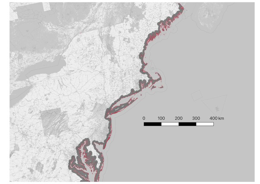
are much more sparsely built; but conditional on SLR-proneness, blocks closer to the coast are more
densely built. Fifth, as we approach the coast, SLR-proneness rises steeply. Sixth, damages from
flooding also rise steeply as we approach the coast. Together, these stylized facts suggest a tension
between the amenity of coastal proximity, and the disamenity of flood-proneness, which increases
steeply near the coast. These two forces balance at a bliss-point: close to the coast, but not too close.
    While the first six stylized facts describe coastal housing around 1990, the last three describe
how it has changed from 1990-2010. Our seventh stylized fact is that despite the considerations
discussed above, much construction near the coast in recent decades took place in areas prone to
SLR (and flooding). As mentioned above, net new construction from 1990-2010 was more than twice
as prevalent in SLR-prone locations as in the 1990 stock of housing. Eighth, SLR-prone areas were
more likely to be developed in dense census tracts, but not in sparse ones. Finally, our ninth stylized
fact is that in the densest census tracts, new construction focused on medium-risk SLR-prone areas,
still avoiding the riskiest ones.
    We show that our nine stylized facts are robust to excluding census blocks, which were mostly
shielded from private residential construction, because they are either protected areas, military bases,
or parks. We also find evidence consistent with our stylized facts when we use data on built area,
which cover all construction rather than just housing data.
    To account for the nine stylized facts, we develop a model of a monocentric coastal city. In the
model, coastal areas are characterized by both an amenity, which declines linearly in the distance
to the coast, and a disamenity (flood-proneness), which declines convexly in distance to the coast.
The city founder chooses a location that trades off these two factors – close to the coast, but not right
at it.4 This location becomes the city’s focal point – the Central Business District (CBD). Residents
then choose where to live, and they prefer locations close to the CBD, both because of their high net
amenity value and because of the shorter commute. Housing density peaks around the CBD, but
declines more steeply on the coast-side, because of the convex flood-proneness. The city expands
over time into previously empty areas on both sides. On the coast side, this expansion involves
building on increasingly flood-prone land.
    After explaining how the model accounts for the nine stylized facts, we extend it in different
ways. Our first extension allows for sea level rise. In the second, we allow for a finite number of
high-elevation areas near the coast, which are safe from flooding. While most locations right by the
coast are still flood-prone (and unpopulated), the handful of elevated locations there command high
prices, consistent with what we see in the data. Third, we allow for costly and irreversible conversion
of land to housing from alternative uses, which makes the developers’ decisions dynamic rather than
static. Finally, we examine government subsidies to flood-prone areas.
    We then simulate our model to explore challenges that low-elevation coastal cities may face in
the coming decades. These simulations point to four potential concerns for low-elevation coastal
cities. First, the problem of housing in flood-prone locations looks set to worsen, either because
cities expand towards the coast, or because of SLR, or because both happen simultaneously. This
development threatens to increase flooding costs for both residents and taxpayers. Second, even if
LECZ cities grow on aggregate, some neighborhoods within them may experience economic decline,
   4 Our model abstracts from productivity differences between locations that are, in any case, close to the coast, but adding

productivity differences does not substantially change the picture.

                                                                 3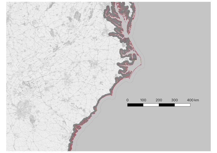
as increased flood risk causes demand for housing to decline. This problem is exacerbated in the case
of economically stagnant cities. Third, SLR further distorts the shape of LECZ cities, significantly
lengthening the time costs of commuting to work. Finally, these cities face a potential crisis if their
CBD comes under threat of being permanently submerged.
    The main contributions of our paper are fourfold. First, we assemble a new dataset on the loca-
tion of housing and flood risk, which covers thousands of kilometers of coast, spanning major urban
centers, small towns, and rural areas. The data, which cover two decades, are at a highly disag-
gregated spatial scale. They include information on housing from the census and land cover from
satellite imagery, as well as measures of SLR-proneness, flood damages, and regulatory restrictions.
These data allow us to explore construction in areas where flood risks for residents and taxpayers
are both high and rising, due to climate change. Second, we use these data to document how the
existing housing stock and new construction vary by distance to the coast. The result is a novel and
detailed picture of housing in LECZ, and its relationship to the vulnerability of different locations to
flooding and SLR. Third, we develop a model, which provides a parsimonious explanation for our
findings. The model answers questions such as: why does housing concentrate near, but not right
at, the coast? Why are coastal cities asymmetric? Why is new housing in LECZ increasingly built
on flood-prone areas, which were previously avoided? And why does this happen especially on the
urban fringes? Finally, we extend our model and use it to study how SLR may reshape cities, and
consider implications for rising costs of flooding and taxpayer subsidies, the economic decline of
some neighborhoods, and lengthening commutes.
    Our paper is related to the literature on the importance of urban amenities (Glaeser, Kolko and
Saiz 2001) and the attraction of coastal areas (Rappaport and Sachs 2003). Though attractive, LECZ
are also prone to flooding, and there are reasons to worry that they might be built over too densely.
First, the flood-proneness of LECZ creates moral hazard, which results in overbuilding when tax-
payers bear some of the costs of reconstruction following floods (Kydland and Prescott 1977) and
of public construction of flood defences. Second, flood risk may be under-appreciated by residents,
because official flood maps do not fully reflect current and future risks (US Department of Homeland
Security 2017), or because people are myopic (Burningham et al. 2008 and Pryce et al. 2011).5 Our
paper identifies a third reason why people build in flood-prone coastal areas: to reduce commuting
costs to jobs in major city centers, which are often near the coast.
    Our paper is also related to the literature on physical barriers to city growth. Building on Saiz
(2010), who studies "hard" physical barriers to city growth, we characterize "soft" barriers, such as
flood-prone areas. Soft barriers are locations that are not used for housing development in most cir-
cumstances, but are nevertheless built on as cities expand. Construction on soft barriers may involve
risks not only to residents but also externalities (e.g., for taxpayers or the environment), which may
necessitate policy intervention.6 Also closely related is Harari (2020), who studies how physical bar-
riers distort the shape of cities and lengthen commutes. Our paper differs in its geographic focus
(the US as opposed to India), and more importantly in its study of flooding and SLR, which further
distorts the shape of coastal cities.
  5 Ortega  and Tas.pınar (2018), Gibson and Mullins (2020), Hino and Burke (2020), and Keys and Mulder (2020) explore
the updating of house prices following information on flooding and SLR.
   6 Construction in areas prone to wildfires is another example of soft barriers.

                                                             4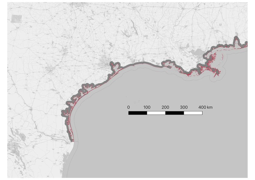
Another related paper is Magontier, Solé-Ollé and Viladecans-Marsal (2019), who study political
economy of coastal destruction in Spain. We differ in our focus on market forces (rather than the
political economy), and in our study of the role of SLR.
Whereas Balboni (2020) studies exposure of Vietnam roads to SLR, we focus on internal city de-
velopment (rather than on intercity roads), and how it evolves in the US. Other economic studies
of the consequences of SLR include Hallegatte et (2013) and Desmet et al. (2021), who quantify its
global costs. Our paper differs in its study of urban structure and how cities may expand even as sea
levels rise.
Finally, our paper is also related to the literature on path dependence in city location (Bleakley
and Lin 2012) and the adaptation of cities to large-scale environmental shocks, such as Hornbeck
and Keniston (2017) and Kocornik-Mina et al. (2020). Our contribution here is to explore how coastal
cities evolve and how SLR reshapes them.
2 Data
2.1 The area and units of analysis
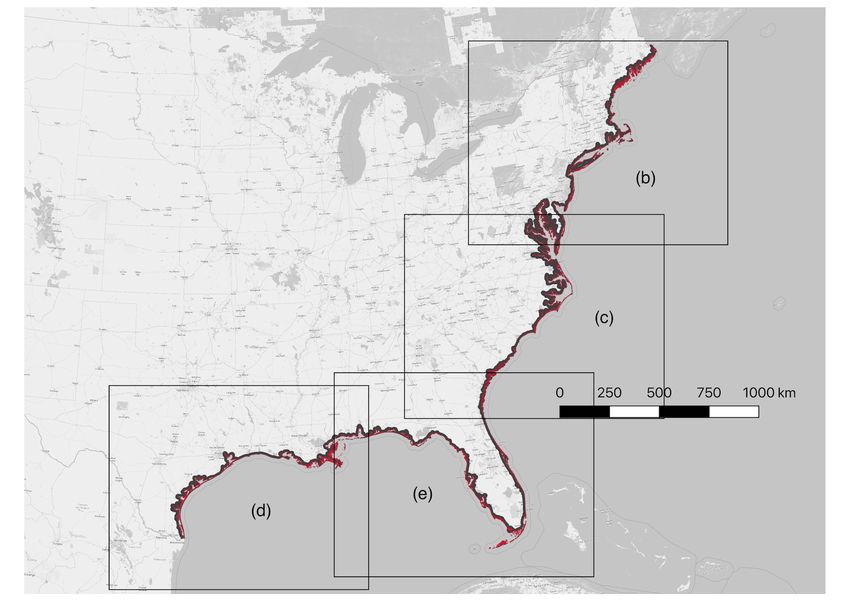
In our analysis we focus on areas within 10km of the US Atlantic and Gulf coasts. This choice of area
reflects a tradeoff between three considerations: a focus on flood-prone and SLR-prone LECZ; an
analysis of fine spatial units; and computational constraints. First, we are interested in low-elevation
coastal zones, and especially those that are prone to flooding and vulnerable to sea level rise. The
area that we study spans the coastal edges of the Atlantic Coastal Plain and the Gulf Coastal Plain,
both of which include many low-elevation coastal locations. The area that we study is highly prone to
flooding: it held 1.7 percent of US housing units in 1990 (and about 2 percent in 2010), but accounted
for 36 percent of the value of National Flood Insurance Program (NFIP) claims from 1973-2019. This
area also experienced some of the fastest rates of local sea level rise in the world during the 20th
century, a trend which is expected to continue and raise the frequency and severity of floods in these
locations (Dahl et al. 2017).
Second, we analyze small spatial units, where the intersection of flood-proneness and construc-
tion can be pinpointed. Much of our analysis is at the level of census blocks – the smallest geographic
units used by the US Census Bureau.7 We also make use of more aggregated geographic units, in-
cluding census designated places (to study the asymmetry of coastal places), and census tracts (the
finest disaggregation for which we have data on damages from floods from the National Flood Insur-
ance Program). The blocks and other geographical units that we use are from the 1990 census, with
later data matched onto them, as detailed below and in the Data Appendix. All the census datasets
that we use are sourced from the NHGIS data archive (Manson et al. 2019).
Finally, we face computational constraints in processing high-resolution data covering such a
large area. Since, as we discuss below, SLR-prone land and NFIP damages are heavily concentrated
within one or two km of the coast, we decided not to explore the area further inland than 10 km.8
7 We complement our census block data with a gridded dataset of 150m x 150m cells, which is the approximate size of
the median census block. More details on this alternative dataset are included below and in the Data Appendix.
8 The only exceptions where we show areas further inland than 10 km are in a few illustrative examples in our appendix,
5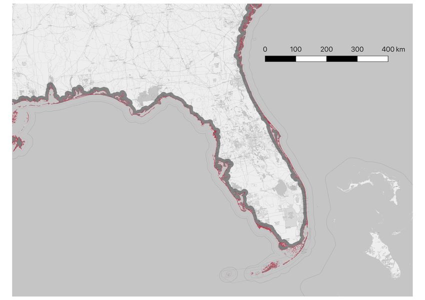
A map of the area that we study is shown in Appendix Figure A1.9 Since the coast is not straight
but winding, the area within 0-1 km of the coast is larger than the area within 1-2 km of the coast,
and so on. In our analysis we take this into account, as we explain below.

2.2     Main outcomes: housing and land cover data

Our housing data come from the US Census and Annual Communities Survey, observed in 1990 and
2010.10 We harmonize all our census data to the geographical units (block boundaries) of the 1990
census, with 2010 data matched to 1990 in proportion to area shares, as described in detail in the
Data Appendix. Our main dataset, composed of census blocks within 10km of the US Atlantic and
Gulf coasts, includes some 544,065 observations, covering a total area of 128,757 sq km. The median
area of blocks in our data is 0.021 sq km (like a square with 145 meters on each side), and the median
number of housing units per block in 1990 is 12. At the level of blocks, we observe the number of
housing units and the median price of owner-occupied dwellings (housing units).11
      As an alternative measure of the extent and intensity of development in coastal areas, we use
land cover data based on Landsat Thematic Mapper (TM) satellite imagery (NOAA 2021). The Land-
sat data come in the form of a raster dataset where each 30m x 30m observation (or pixel) has been
assigned to one of 25 land cover categories.12 In our analysis, we focus on the four developed cat-
egories, which represent different extents of constructed surfaces (including buildings, roads, and
parking lots).13 For computational reasons, we aggregate the Landsat data to 150m x 150m cells (the
approximate size of the median census block in our data), taking the midpoint values of the four
developed categories to arrive at a measure of the fraction of each cell’s land area that is developed
(i.e., covered in constructed materials). We observe this variable in 1996 and 2010, the earliest and
latest years for which we have complete Landsat data.14

2.3     SLR data

Our data on sea level rise come from detailed maps of areas anticipated to be inundated for various
future sea level rise scenarios, which we obtained from NOAA’s digital coast platform (Marcy et
al. 2011). These maps show inland extent of inundation for scenarios of sea level rise from 0 to 6
as discussed below. Our economic analysis consistently focuses on the area within 10 km of the coast.
   9 We use the Database of Global Administrative Boundaries (GADM 2018) to define the coast. This shapefile includes

sections of major rivers, such as the Charles in Boston, East River and the Hudson River in New York City, and the Potomac
in Washington, DC, as part of the coastline. But lakes and upstream sections of rivers are typically excluded from the coast
shapefile, and consequently Philadelphia, New Orleans, and Houston, are largely outside our dataset. Overall, the area
we study consists of parts of 18 states and the District of Columbia, as listed in the Data Appendix.
  10 What we refer to as “2010” is more precisely data for 2006 - 2010 from the Annual Communities Survey.
  11 Just over a fifth (22.4%) of blocks in our sample were empty - i.e. had zero housing units - in 1990.
  12 These categories include various classifications of open water, wetlands, agricultural land, forest etc., as detailed here:

https://coast.noaa.gov/digitalcoast/training/ccap-land-cover-classifications.html.
  13 The four developed categories in the Landsat data are: “developed - high intensity” where constructed materials

account for 80 to 100 percent of the total cover at that location; “developed medium intensity” (50-79 percent constructed
material); “developed - low intensity” (21-49 percent); and “developed - open space”, where constructed material accounts
for less than 20 percent of land cover.
  14 Our cells dataset includes over 6 million observations, or cells within 10km of the Atlantic and Gulf coasts. The mean

share developed in 1996 is 0.066. More than 70% of cells in our data have share developed = 0 in 1996. By construction, the
share developed measure is top-coded at 0.9, but there are fewer than 7,000 cells in our data with this value for developed
share in 1996.

                                                                  6
feet. Importantly, the mapping process also takes account of major federal leveed areas, which are
assumed, for the purposes of creating these inundation maps, to be high enough and strong enough
to prevent inundation, regardless of the SLR scenario.15
In our analysis we focus on the share of an area (e.g., a block), which would be under water at
high tide if SLR is 1 foot (approx. 30.5cm). Information on sea level rise was added to the blocks (and
cells) by intersecting the shapefiles for blocks (cells) with shapefiles of areas expected to be inundated
for 1ft of sea level rise using GIS software. We then calculate the share of each census block (or cell)
that is exposed to 1ft of sea level rise, which we refer to as SLR1 f t. We further define low-risk areas
as blocks (or cells) in our data where SLR1 f t = 0; medium-risk, where SLR1 f t 2 (0, 0.5]; and high-
risk, where SLR1 f t 2 (0.5, 1]. Of the blocks in our sample, 86% are low-risk. Overall, the mean share
1ft SLR for the entire sample of blocks is 0.045, and the area-weighted mean share is around 0.18.16
2.4 Building restrictions
Our dataset also includes information on areas where building construction may be restricted. While
such restrictions may be an endogenous response by governments at different levels to the danger
of building close to the coast, we nevertheless examine the role that such regulations may have in
our setting. Here we discuss three different types of regulations: restricted areas, where housing
development may be particularly constrained; state "setback lines" close to the coast, beyond which
construction may be more regulated; and local government regulations on building density.
We begin by gathering data on what we refer to as restricted development areas – i.e. areas
where development is likely to be prohibited or highly constrained, for one of three reasons: due to a
protected areas designation, including for conservation, natural resource management or recreation
(e.g. the Everglades in Florida); because of the presence of a city park (e.g. Central Park in New
York City or Boston Common), or where land is owned by the military (e.g. Norfolk naval base in
Virginia). As a robustness check, we replicate all our main findings excluding blocks (or cells) where
50% or more of the land area is accounted for by the sum of any of these three restricted development
areas. While blocks that meet our restricted development area criterion make up just 3.5% of the
observations (18,863 blocks), they account for a sizeable share of the total land area in our sample
(over 19%). The vast majority (over 88%) of the land area in our sample that we identify as restricted
for development is accounted for by areas that have been designated as protected. New development
in restricted areas is quite limited – some 90,000 new housing units were added to blocks with at least
50% land area restricted for development between 1990 and 2010, compared with 3.24 million new
housing units across all blocks in our sample. Full details of the data sources and definitions used to
identify restricted development areas are included in the Data Appendix.
Another factor which may influence construction is the existence of "setback lines", which are
designed to protect fragile environments close to the coast. Unlike the EU and other countries, the
US does not have a federal "setback line", which prohibits construction within a fixed distance of the
shoreline (Simpson et al. 2012). Instead, there are setback lines in some states.17 The geographic
15 The SLR maps assume that New Orleans is safe even from 6-foot of SLR.
16 A recent study has suggested that many areas on US Atlantic and Gulf coasts could experience 1ft SLR as early as 2045
(Dahl et al. 2017).
17 Of the states in our dataset, Alabama, Delaware, Florida, Georgia, Maine, New Hampshire, New Jersey, New York,
7location of those lines differs both between and within states, but in many cases they appear to
be drawn within a few tens of meters of the coast. Construction is not necessarily banned even
beyond setback lines, but it may be more regulated. While we have no shapefiles showing the areas
covered by these lines, we have examined the lines themselves in one state of particular importance –
Florida.18 Much of Florida’s line (Coastal Construction Control Line Program 2021) runs near the sea-
facing edge of its barrier islands, leaving many SLR-prone areas open to construction. And visual
inspection shows that there are buildings even beyond that line. Nevertheless, it is likely that the
existence of "setback lines" contributes to the low housing density in the immediate vicinity of the
coast.
Moving from state regulations to the more local level, we consider housing market land restric-
tions on building density. Specifically, we use Density Restriction Index (DRI) from the Wharton
Residential Land Use Regulation Index (Gyourko et al. 2019). Since these data are at a different level
of aggregation than the one we use, we aggregate them to the county level, and match them to our
block-level data.
2.5 Additional data sources
Besides the datasets discussed above, other data used in our analysis include information on census
designated places (both polygons and points), sourced from the NHGIS data archive (Manson et
al. 2019), which we use to define place extents and the location of the CBD of each place. NHGIS
assigns place points based on the Geographic Names Information System (GNIS) coordinates of each
place’s historical or functional center (typically the central business district). Other characteristics of
places – e.g. their size and asymmetry – are calculated based on information from blocks aggregated
to places. Specifically, we define place size in two ways: one is the linear distance j x L x R j, where
x L is approximated as the minimum distance to coast from the centroid of any block in a place, and
x R the maximum distance to coast from the centroid of any block in the same place; the other is the
j x R x0 j
sum of the area of blocks in the place. Place asymmetry is defined as the ratio of distances jxR xL j
,
where x0 is distance to the coast from the CBD.19
Data on historical damages from coastal flooding are taken from the National Flood Insurance
Program (NFIP), operated by FEMA, which subsidizes flood insurance provision. In particular, we
use data on insured losses from coastal floods, available at the census tract level, from 1973 to 2019.
There are two points to note about NFIP. First, NFIP includes an implicit subsidy component. For
example, the Congressional Budget Office (CBO 2017) notes that in 2016, “the overall shortfall of
$1.4 billion is attributable largely to premiums’ falling short of expected costs in coastal counties,
which constitute roughly 10 percent of all counties with NFIP policies but account for three-quarters
of all NFIP policies nationwide . . . the net short- fall measured over all coastal counties is $1.5 bil-
lion, whereas the net surplus measured over all inland counties is $200 million.” A recent analysis
concluded that while NFIP’s shortfalls cannot be attributed to any single incident, it borrowed sig-
North Carolina, Pennsylvania, Rhode Island, South Carolina, Texas, and Virginia have setback lines (Simpson et al. 2012).
18 Even in the case of Florida we do not have the shapefile of the restricted area, but only of the line itself.
19 While asymmetry is generally on the interval (0, 1), space is two-dimensional, so in principle it may exceed 1 in
some cases. In practice there are fewer than a handful of such cases, and excluding or Winsorizing them at 1 makes no
appreciable difference to the results.
8nificantly following Hurricanes Katrina in 2005 and Sandy in 2012. In 2017, as NFIP reached its
borrowing cap of $30.5 billion, Congress canceled $16 billion of its liabilities, to allow NFIP to bor-
row more in response to Hurricanes Harvey, Irma, and Maria (Peterson Foundation 2020). It is also
noteworthy that by our estimates, claims made to NFIP grew at a rate of around 4-5 percent in real
terms from 1978-2019.20
While claims made under the NFIP by no means capture the totality of economic losses from
coastal floods (or in fact the totality of residential losses from flooding, as some damage is unin-
sured), the NFIP data have the advantage of being available at a relatively fine level of geographic
disaggregation – the census tract level – which makes these data well suited to our task of estimating
how damages from flooding vary with distance from the coast. We convert these claims data to 2020
US dollars and aggregate the damages data across the entire period available (1973-2019).21 We also
normalize the figures by dividing the damages by the number of housing units in each tract from
2014-2018 (Manson et al. 2019).
Information on public spending associated with coastal flooding, which we use to calculate the
share of damages subsidized by the taxpayer, was largely sourced from a recent Congressional Bud-
get Office report (CBO 2019). This report estimates that $19.4 billion of taxpayer money is spent
annually on mitigation of and relief from the damages caused by hurricanes.
Additional data sources used for our model simulation are detailed in Appendix Table A5, and
we discuss the parameter estimates themselves in Section 4.5.1.
3 Empirical findings
This section documents nine stylized facts about the location of housing and its exposure to flood
risk and sea level rise, focusing on the area that lies within 10 km of the US Atlantic and Gulf coasts,
as discussed in Section 2. This section consists of three parts. First, we discuss three stylized facts that
characterize housing and places near the coast in the cross-section; second, we discuss three stylized
facts that begin to reveal why housing near the coast follows the patterns that we document; and
finally, we show three stylized facts on the development of coastal housing over time.
3.1 Stylized facts on the cross-section of coastal housing
The first stylized fact we document is that housing unit density peaks near – but not right at –
the coast. To show this, we calculate the number of housing units in each 150 meter distance bin
from the coast, assigning the housing units in each census block to the bin where its centroid falls.
We then normalize the total number of housing units in each bin by the area of that bin, which we
approximate using the cells.22 The results, in Panel (a) of Figure 1, show that the logarithm of housing
20 NFIP claims were significantly lower before 1978. When we use all the data from 1973-2019, we find an even higher
growth rate of around 10-12 percent.
21 All dollar values used in our analysis, except where otherwise stated, are normalized to 2020 US dollars, using a GDP
deflator (Federal Reserve Bank of St. Louis 2020).
22 Census block centroids provide a good approximation of housing location, since areas with dense housing are parti-
tioned into small blocks. But block centroids are less precise when it comes to measuring area, because areas with sparse
housing (or no housing) tend to be in large census blocks. Using cell data to approximate land area in each distance bin is
therefore more reliable, since the cells are by construction evenly distributed, and of equal size.
9unit density peaks around 2.475 km from the coast, and declines asymmetrically, falling more rapidly
on the coast side.23 Specifically, housing density declines steeply as we approach the coast (falling
about 0.55 log points over less than 2.5 km) and more slowly on the inland side (falling about 0.85 log
points over about 7.5 km). A similar pattern can be seen in Panel (b) of Figure 1, which restricts the
analysis to census blocks with housing units, and reports point estimates and 95 percent confidence
intervals from estimating the regression:
ln (hdensityi ) = β11 + β12 Bini + e1i , (1)
where hdensityi is the number of housing units per square km in census block i, Bini is a vector of
indicators for 50 meter distance bins from the coast, and e1i is an error term, which is clustered by
state here and in all the spatial regressions we report below.24 The figure peaks around 3km from the
coast, and declines on both sides of the peak, again with a steeper decline on the coast side. As we
discuss below, the steep decline near the coast side of Panel (b) understates the sparseness of housing
density near the coast, since there are more empty blocks in the immediate vicinity of the coast; for
that reason, we prefer the specification in Panel (a). We repeat the analysis of the two panels above
in Panels (a) and (b) of Appendix Figure A2, this time excluding restricted areas (as discussed in the
Data Section).25 The results are largely unchanged.26
Panel (c) of Figure A2 repeats the analysis of panel (a) of Figure 1 but using only block-level data,
for area as well as housing units. Here the decline in density near the coast is even steeper.27 Finally,
Panel (d) of Appendix Figure A2 repeats the analysis of panel (a) of Figure 1 using cell-level data
on built area instead of housing units. Using the built area data allows us to examine the extent
not only of residential housing, but also of commercial and industrial areas, as well as roads and
other artificial structures. Here the distribution peaks around 2km from the coast, and once again the
decline on either side is asymmetric and similar in magnitude to that in Figure 1.
In interpreting the above-mentioned housing distribution, it is worth noting several additional
empirical regularities. Commuting remains an important aspect of cities, and the vast majority of
housing units that we consider are primary residences, where people work throughout most of the
year.28 Specifically, only around 1 percent of the housing units in our sample are second homes.29
23 Housing density is quite similar to the peak in other nearby distance bins, and it displays some geographic variation.
Specifically, in the US South, housing density peaks closer to the coast, consistent with a higher amenity value of the beach.
But in every case we examined, density falls steeply very close to the coast and more gradually further away from it.
24 This approach follows Donaldson and Hornbeck (2016) and others. We explored using spatial clustering following
Bester, Conley, and Hansen et al. (2011), using 1 x 1 degree clusters. This gave slightly smaller standard errors than those
we report. Using Conley (1999) standard errors is more technically challenging in our setting, due to the large number of
observations.
25 As discussed in Section 2, we have no data on the location of all setback areas where construction is more regulated.
Their existence may contribute to the steep fall in housing density within around 150 meters from the coast, but is unlikely
to drive the overall pattern where housing density peaks around 2-3 km from the coast.
26 Similarly, controlling for the Density Restriction Index (DRI) has little impact on the patterns shown in Panel (b) of
Figure 1 (results available on request).
27 As discussed above, this may be related to a less precise measurement of area using the block-level data, whose sizes
are uneven.
28 At the same time, the very recent rise in the popularity of telecommuting may suggest that there will be less physical
commuting in the future.
29 While the share of second homes rises in the immediate vicinity of the coast, it is still less than 7 percent even there.
We also note that mobile homes make up only around 5 percent of our sample.
10Since we do not have fine-grained data on business activity, we assume in the discussion below that
peak housing density corresponds to the location of the Central Business District (CBD). We note
that given the limitations of our data we cannot explore multiple employment centers within the
city, although we discuss this possibility below.30
Our second stylized fact is related to the first, namely that census-designated places close to the
coast are asymmetric.31 To show this, we use data on places and their CBDs to estimate regressions
of the form:
asymmetry j = β21 + β22 Bin j + e2j .
j x R x0 j
Here asymmetry j is the ratio jxR xL j
, where the numerator is the distance from each place’s furthest
point from the coast to its CBD, and the denominator is the distance from each place’s furthest point
from the coast to its nearest point to the coast; Bin j is a vector of indicators for 1 km distance bins
from the coast; and e2j is an error term.32 As Table 1 shows, places whose centroids are within 4km
from the coast are asymmetric: the distance from their CBD to their inland edge is roughly double
the distance from their CBD to the coast side edge. In contrast, places around 4-10km from the coast
are roughly symmetric. An example of this can be seen in Appendix Figure A3, which shows places
in the Greater Boston area: those close to the coast are asymmetric, while those further away are
more symmetric.
The third stylized fact is that the asymmetry near the coast is more pronounced for large places.
We show this by using the place-level data to estimate regressions of the form:
asymmetry j = β31 + β32 size j + β33 ln dist_coast j + β34 size j ln dist_coast j + e3j , (2)
where size j measures the size of place j, either as ln area j where the area is in square kilometers
or as the distance j x R x L j in km; dist_coast j is the mean distance from each place’s blocks to the
coast; and e3i is an error term. The estimates in columns (1) and (2) of Table 2, which add the re-
striction β33 = β34 = 0, show that on average, larger places (using either of the above measures) are
more asymmetric. Columns (3) and (4), which are unrestricted, show that the asymmetry is more
pronounced for large places when their CBDs are closer to the coast.
3.2 Stylized facts on mechanisms that shape the coastal housing distribution
Whereas the three stylized facts above tell us how economic activity concentrates near the coast, the
next three tell us something about why this is the case. Our fourth stylized fact is that blocks that
are highly prone to sea level rise (SLR) are less densely built, but conditional on SLR-proneness,
blocks closer to the coast are more densely built. To show this, we focus on the share of the area of
each census block, which will be under water at high tide if sea level rise (SLR) were 1 foot, or 0.305
30 The equivalent figures to Panels (a) and (b) for 2010 reveal a very similar picture; the peak of the housing density
moves 300 m inland in the 2010 equivalent of Panel (a) but stays constant in the equivalent of Panel (b). In Section 4.5.2 we
consider cases where the CBD moves over time.
31 Census-designated places are numerous and we have data on their CBD location. Many of them are contained within
the area of our study, even if metropolitan areas as a whole extend further inland.
32 Our asymmetry measure, j XR X0 j , is for the most part, bounded on the interval [0,1]. There is a small minority of cases
j XR XL j
where the measure exceeds 1, since in reality XR , X0 , and X L are not all on one line. Nevertheless, excluding these few
cases does not substantively affect our estimates.
11meters (we refer to this share as SLR1 f t). In interpreting SLR1 f t we note that it matters not only
for a future with higher sea levels, but also for the present: areas with high SLR1 f t are more prone
to both frequent low-intensity "nuisance flooding" and to flooding from impactful events, such as
tropical storms (Dahl et al. 2017). Therefore, all else equal, living in areas with high SLR1 f t likely
involves costs (a point which we revisit below), and can be viewed as a disamenity. To examine how
much these areas are avoided, we split the census blocks into three groups: high-risk medium-risk,
and low-risk, as discussed in Section 2. We then repeat the analysis in Panel (a) of Figure 1 separately
for each of the three groups of blocks.33 The results in Figure 2 show that at every distance bin from
the coast, low-risk census blocks are about two to three times more densely built than medium-risk
blocks, while the medium risk ones are, at most distance bins, several times denser than the high-risk
ones. These results are confirmed in robustness checks that we report in Figure A4, where we repeat
the analysis in Figure 2 excluding the restricted areas (Panel (a)) and then using the fraction of cell
area that is built, based on our gridded data (Panel (b)). When we look within each of the three risk
groups, housing density tends to increase as we approach the coast. In other words, conditional on
the level of risk, proximity to the coast seems like an amenity.34
As our fifth stylized fact shows, however, as we approach the coast, SLR-proneness rises steeply.
We show this in two ways in Figure 3. As Panel (a) of Figure 3 shows, the fraction of blocks that are
low risk is fairly stable at well over 90% in the area 3-10km from the coast. In the three km closest
to the coast, however, this share declines, slowly at first and then rapidly, reaching less than 20% as
we get very close to the coast. Over the same range the share of medium risk rises from less than
10% to almost 50%. Meanwhile, the share of high risk, which is less than 10% even a few hundred
meters from the coast rises even more sharply to almost 40% very close to the coast. Panel (b) of
Figure 3 reports the mean SLR1 f t by distance to the coast. This share is lower than 5% in the area 1-
10km from the coast, but increases steeply to almost 45% as we get very close to the coast. Appendix
Figure A5 shows that these results are again robust to excluding restricted areas. Together, this
evidence suggests that the amenity of proximity to the coast, which increases gradually (as we saw
in the fourth stylized fact), is offset by a convex disamenity due to flood risk as we near the coast.
To see why this matters, we turn to the sixth stylized fact: damages from flooding rise steeply as
we approach the coast. To show this, Figure 4 reports point estimates and 95% confidence intervals
from the regression:
ln (damagek ) = β41 + β42 Bink + e4k , (3)
where damagek is the total dollar sum of NFIP claims from 1973-2019 (in 2020 USD), normalized
by an estimate of the number of housing units from 2014-2018 in census tract k; Bink is a vector of
indicators for 150 meter distance bins from the coast; and e4k is an error term.35 As the figure shows,
claims in the distance bin closest to the coast are about 2.5 to 3 log points (or about 12-20 times) higher
than in the areas around 4-10km from the coast. While NFIP claims represent only a fraction of the
33 Except this time we use area data from the blocks.
34 Since we restrict our analysis to areas within 10 km of the coast, we abstract from differences in productivity across
locations. We revisit this point in our discussion of the model.
35 The use of the recent housing units measure mitigates the risk that NFIP claims per housing unit will appear large
near the coast because housing expanded there, as we discuss below. The patterns we document are, however, robust to
using 1990 housing units in the denominator.
12total costs of flooding over the past few decades, this figure indicates that flood costs rise convexly
as we approach the coast.36
Having characterized the first six stylized facts, we now examine the distribution of prices near
the coast. Panel (a) of Figure A6 reports estimates using the same specification as Panel (c) of Figure 1,
except plotting the fraction of blocks in each 50-meter distance bin from the coast, for which median
house prices are missing. Median prices are missing if blocks are empty or very sparsely populated,
so that disclosing moments from the price distribution would reveal information about individual
housing units. The figure shows that median house prices are missing for about 30 percent of the
census blocks from around 1-10 km from the coast. In the 1 km closest to the coast, however, the
fraction missing rises steeply, to almost 67 percent in the blocks closest to the coast. Panel (b) shows
that where median house prices are available, they are also fairly flat around 1-10 km from the coast,
rising steeply in the 1km closest to the coast. Interpreting this pattern is not straightforward, because
of the missing blocks; the coverage within blocks (only 64.1% of housing units in 1990 were owner-
occupied); differences in housing characteristics within locations and across them; and the use of
the median. Nevertheless, at first glance, the findings we document may seem surprising: blocks
near the coast are flood-prone and much sparser than others, and this sparseness is not driven by
restricted areas, as Panels (a) and (b) of Figure 1 show; yet where house prices are recorded there,
they are high. We explain this apparent puzzle in Section 4.4.3, by noting that while locations in
blocks close to the coast are generally flood-prone and therefore in low demand, there may be small
higher-elevation areas within these blocks, where flooding is much less of a problem, and where
prices are high.
Returning to our first six stylized facts, we note that stylized facts 4-6 help explain stylized facts
1-3: conditional on risk, people seem to prefer to live as close as possible to the coast, but as we
approach the coast risks increase steeply. This gives rise to the distribution of housing density, which
peaks near the coast and declines asymmetrically, falling more steeply on the coast side than on the
inland side.
3.3 Stylized facts on changes in coastal housing over time
Whereas the first six stylized facts describe coastal area housing at a point in time, mostly around
1990, the last three stylized facts describe how they changed from 1990-2010. The seventh stylized
fact is that despite the risks discussed above, much construction near the coast in recent decades
took place in areas with SLR risk. This is shown in Table 3. In 1990, areas with medium or high SLR
risk accounted for about 12% of the housing units in our area of study, and this fraction increased to
around 14% in 2010. This came about because 26% of the net increase in housing units in the area we
study from 1990-2010 took place in medium or high-risk blocks.
The eighth stylized fact tells us where the risky new developments took place: SLR-prone areas
were developed in dense census tracts, but not in sparse ones. Table 4 reports regression estimates
using the specification as in (1), except that the dependent variable is the change in housing units
36 Aswe discuss in the Data Appendix, NFIP costs cover only a fraction of total damages from flooding. We use it here
because it affords spatially disaggregated data at the level of census tracts. Since census tracts are considerably larger than
blocks and focus on built areas, there is no point in excluding restricted areas at this level of the analysis.
13in each census block from 1990-2010 and the regressor is SLR1 f t. These regressions are estimated
separately for four groups of census blocks, grouped by the housing density of the census tracts that
contain them (where this density excludes the own block’s density). As the table shows, in sparse
census tracts, the growth in housing units is negatively associated with SLR. But in dense census
tracts, new construction is positively associated with SLR proneness (although these estimates are
only marginally significant). All this suggests that where there is plenty of space to build, SLR-prone
areas are avoided, in line with the evidence discussed above; SLR-prone areas are, however, built on
in dense areas, presumably because no other local alternatives exist. We repeat this analysis exclud-
ing the restricted areas (Appendix Table A1) and the results are largely unchanged. We then repeat
the analysis again using the cell data on built area, where this time "neighborhoods" are larger (1
square km) areas, whose fraction built we calculate excluding the own cell. In this case the estimates
in sparse "neighborhoods" are again negative, while in the densest category the estimates are pos-
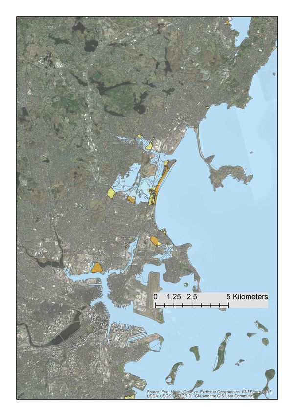
itive but imprecise. Appendix Figure A7 shows four case studies, which illustrate development in
the fringes of dense tracts: Revere and Chelsea in Greater Boston, Massachusetts; Jamaica Bay and
Rockaway Peninsula in the borough of Queens, New York City, New York; Miami Beach and Miami,
Florida; and Clearwater and Largo, Tampa Bay area, Florida.
Finally, our ninth stylized fact is that in the densest census tracts, new construction focused on
medium-risk rather than high-risk areas. To show this, Table 5 reports estimates from two regres-
sions, which restrict the analysis to the densest group of census tracts discussed above. Column (1)
uses specification (1), but with the change in housing units in each census block from 1990-2010 as
the dependent variable and an exhaustive set of bins for different percent SLR in each census block.
Column (2) is the same, except that the regressors are an indicator ISLR1 f t>0 (that is, medium or high
risk) and a continuous measure (SLR1 f t). Both specifications tell a similar story: new construction
took place in medium-risk areas more than in low-risk areas, but the highest risk areas were still gen-
erally avoided. Appendix Table A3 repeats this analysis, excluding restricted areas, and the results
are largely unchanged. Appendix Table A4 repeats the analysis, this time using the cells instead of
blocks (as discussed above), and the results are again similar to those in Table 5.
4 Model
4.1 Baseline assumptions
In this section, we present a model on coastal development that helps to reconcile the nine stylized
facts that we documented above. The model is in discrete time, and periods are denoted by t. Spa-
tially, we extend the monocentric city model (Alonso 1964, Mills 1967, Muth 1969), by placing it in
the context of a coast, proximity to which offers both benefits and costs.37 The key geographic lo-
cations of the city are the CBD, denoted by x0 ; the coast-side and inland edges of the city, denoted
37 The monocentric city model is commonly used in urban economics. While it abstracts for the multiplicity of employ-
ment locations within cities, it has useful comparative statics and strong empirical support (e.g., Duranton and Puga 2014).
Moreover, when adapted as we describe below, it neatly and parsimoniously explains our findings. Nevertheless, the
existence of multiple employment centers within cities may mitigate some of the distortions that we document.
14by x Lt and x Rt ; and the coast itself, whose initial location is normalized to 0.38 Initially, the CBD
location is chosen by a historical city founder, and then the city persists for T periods (decades). In
each period, developers choose where to build, taking into account the preferences of residents, who
choose where to locate.
The city founder is assumed to be myopic, and chooses a location x to maximize their locational
utility
U F (x) = θ1 x θ2 x σ
. (4)
We assume that θ 1 > 0,reflecting our observation that proximity to the coast has an amenity value
(air, views, bathing), which we assume is linear.39 We also assume θ 2 > 0 and σ > 0, reflecting a con-
vex disamenity (higher risk of flooding).40 As we discuss further below, housing density increases
and then decreases as we head inland from the coast, which is consistent with a demand-based ex-
planation. We note that for simplicity, the model is deterministic, and the risk of flooding is captured
by the last term of the utility function. We assume that the founder’s chosen location becomes the
city’s CBD, x0 .41
There is a continuum [0, x ] of competitive and forward-looking developers, each of whom owns
a plot of land of measure 1 in location x.42 Each period, each developer can allocate their plot to
housing, which yields a period price of pt ( x ), or to agriculture, which has a period price p A .43 The
developers’ time preference is captured by δ 2 (0, 1), and in each period every developer maximizes
their present-discounted stream of future prices.
Finally, there is a continuum of perfectly mobile residents. In every period t = 1, .., T, each
resident may live in the city or outside it.44 If they live in the city, they inelastically supply one unit
of labor, receive a wage, and spend their income on consumption and housing, in which case their
utility is:
U (ct , ht , x ) = cαt h1t α
θ1 x θ2 x σ
(5)
where ct denotes private consumption goods and ht denotes housing in period t and α 2 (0, 1) is the
consumption share of income.45 We assume that residents’ preferences satisfy standard assumptions
(Uc > 0, Uh > 0, Ucc < 0, Uhh < 0). The residents’ locational preferences are the same as those of the
city founder. The budget constraint of each resident in period t is:
38 Later, when we explore SLR, we relax this assumption by allowing xct to grow over time. All our analysis focuses on
inland locations (x > xct ).
39 It is possible that across wider areas than the coastal band that we study, the amenity component of the utility function
also declines convexly in distance to the coast. But the key assumption is that it is less convex than the disamenity term,
so for simplicity we assume a linear amenity term in the vicinity of the coast, which is the area we focus on. As we discuss
below, this assumption is motivated by the convex increase in flood risk as we near the coast.
40 We focus on the negative consequences of flooding, but the disamenity modelled here may include indirect effects of
flooding on the soil’s suitability for housing, as well as the effects of wind gusts.
41 The location of many cities on the US Atlantic and Gulf coasts was established more than a century ago, so for simplic-
ity we assume that their location choices were myopic. We also ignore any productivity component in the city founder’s
locational choice, although adding this would not make much difference to the model overall.
42 We assume that x > 0 is sufficiently high not to constrain the coast side development.
43 We follow the literature by labelling non-housing use as agriculture, although in practice there may be other alternative
uses of land. In the baseline model we assume that agricultural prices are fixed across time and space, and that there is no
cost of converting land across uses. We relax the latter assumption in an extension in Section 4.4.2. One caveat that we do
not consider is salinity, which may affect some forms of agriculture, but not others (e.g., fishing).
44 We assume that there are more than enough residents to populate the city at each point in time.
45 There are no savings in the model.
15p t ( x ) h t + c t = wt jx x0 j (6)
where the price of consumption is normalized to 1; wt is wage, and j x x0 j reflects the time cost of
commuting. Each resident also has an outside option of living outside the city, with utility Ū > 0. We
initially consider a city whose attractiveness to residents and developers increases (at least weakly)
relative to the outside option, or in other words that wt increases (weakly) in t.
We solve the model as a Nash equilibrium, where developers take into account the expected
maximization of other developers and of the residents.
4.2 Equilibrium
Here we summarize the equilibrium conditions of the model, a visual illustration of which is dis-
cussed in Section 4.5.2.
City founder: maximization of the city founder’s decision implies, using the first-order condition,
that 1
σθ 2 σ +1
x0 = . (7)
θ1
Residents decide where to live and the share of consumption goods and housing in their con-
sumption bundle. In equilibrium they are indifferent between all city locations, including the city
endpoints, and their outside option Ū. Residents’ indifference between locations then determines
the price function, pt ( x ), for each period.
Developers decide which locations should be part of the city, taking into account the present
discounted stream of future prices. Since the baseline setup of the model is static, developers will
build in all locations such that
pt ( x ) pA. (8)
Since (as we show below) prices decrease monotonically as we move away from the CBD, the
boundaries of the city x Lt and x Rt are pinned down by the equations:
pt ( x Rt ) = pt ( x Lt ) = p A . (9)
Note that because of the assumptions discussed above, developers can repurpose land costlessly in
every period, severing any dynamic link between periods. Below we discuss an extension where
housing construction is costly and irreversible, which introduces dynamic considerations.
4.3 Relating the model to the stylized facts
We now discuss how the model rationalizes the nine stylized facts that we observe. We begin with
Stylized fact 4, that flood-prone areas are more sparsely built, but holding flood risk constant prox-
imity to the coast is seen as an amenity. This motivates our assumption that θ 1 > 0. At the same
time, Stylized facts 5 and 6 show that the cost of flooding rises convexly with proximity to the coast,
motivating our assumptions that θ 2 > 0 and σ > 0.
16You can also read


