Identifying suitable multifunctional restoration areas for Forest Landscape Restoration in Central Chile
←
→
Page content transcription
If your browser does not render page correctly, please read the page content below
Identifying suitable multifunctional restoration areas for
            Forest Landscape Restoration in Central Chile
                                 JENNIFER JELENA SCHULZ1,2,        AND             €
                                                                         BORIS SCHRODER 3,4

                  1
                   Institute for Earth and Environmental Science, University of Potsdam, 14476 Potsdam, Germany
                          2
                            Wissenschaftszentrum Weihenstephan fu €r Ern€ahrung, Landnutzung und Umwelt,
                                      Technische Universit€at Mu
                                                               €nchen, 85354 Freising, Germany
                           3
                             Landscape Ecology and Environmental Systems Analysis, Institute of Geoecology,
                                 Technische Universit€at Braunschweig, 38106 Braunschweig, Germany
                  4
                   Berlin-Brandenburg Institute of Advanced Biodiversity Research (BBIB), 14195 Berlin, Germany

Citation: Schulz, J. J., and B. Schr€
                                    oder. 2017. Identifying suitable multifunctional restoration areas for Forest Landscape
Restoration in Central Chile. Ecosphere 8(1):e01644. 10.1002/ecs2.1644

Abstract. Large-scale deforestation has led to drastic alterations of landscapes worldwide, with serious
declines of biodiversity and ecosystem functions, leading to impacts on humanity ranging from the local to
the global scale. However, the provision of crucial ecosystem functions is not only determined by the
extent, but also by the spatial configuration of forests within the landscape mosaic. An approach that aims
to restore forest functions on a landscape scale is Forest Landscape Restoration, with the purpose to regain
ecological integrity and support human well-being. The landscape-scale approach should enhance the con-
tribution of site-based restoration to larger-scale processes and functional synergies. A fundamental chal-
lenge for Forest Landscape Restoration is therefore the identification of restoration areas within the
landscape where multiple functions operating on different scales can be enhanced. Equally important is
the task of identifying areas requiring restoration. Proposed strategies include the assessment of current,
past, and reference landscape states. However, integrative planning approaches combining historical and
functional perspectives on a landscape scale are little developed. In this paper, we demonstrate how forest
restoration areas can be identified that account for historical forest patterns while simultaneously targeting
multiple forest functions. We use a method developed for habitat suitability modeling based on recent his-
torical forest occurrence and regeneration patterns from 1985 to 2008 in order to predict areas that are suit-
able for forest restoration (potential forest growth) as well as areas where forest potentially recovers by
natural regeneration. For both, unsuitable areas are excluded by masking restoration constraints. Sepa-
rately, we map potential forest functions and assess spatial synergies or “multifunctional hotspots” using
spatial multi-criteria analysis. To derive a scenario of potential restoration areas, predicted maps of restora-
tion suitability and regeneration potential are separately combined with a map depicting the degree of
multifunctionality. These maps are finally overlapped to identify multifunctional restoration and regenera-
tion areas. These designated areas are then evaluated regarding their distribution on current land cover
and recent historical deforestation areas. We test this approach for the dry forest landscape in Central
Chile, an international biodiversity hotspot, which has undergone profound historical transformations and
considerable deforestation in recent decades.

Key words: carbon sequestration; ecosystem functions; erosion prevention; Forest Landscape Restoration; forest
regeneration; habitat connectivity; habitat suitability models; historical forest patterns; multifunctional synergies;
restoration planning; spatial multi-criteria evaluation.

Received 5 August 2016; revised 4 November 2016; accepted 9 November 2016. Corresponding Editor: Charles Kwit.
Copyright: © 2017 Schulz and Schr€  oder. This is an open access article under the terms of the Creative Commons
Attribution License, which permits use, distribution and reproduction in any medium, provided the original work is
properly cited.
 E-mail: jennifer.schulz@uni-potsdam.de

              ❖ www.esajournals.org                            1               January 2017   ❖ Volume 8(1) ❖ Article e01644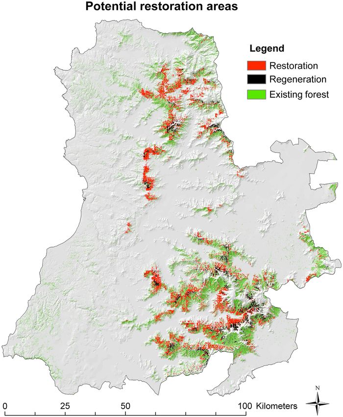
€
                                                                                         SCHULZ AND SCHRODER

INTRODUCTION                                                 regional and landscape scales (Zhou et al. 2008,
                                                             Orsi and Geneletti 2010).
   The magnitude of landscape transformations,                  Whereas traditional restoration approaches set
historically containing a large share of natural             their goals according to historical reference states
perennial ecosystems, to intensively used and                to recover ecosystems and their biodiversity (e.g.,
partly degraded land has serious consequences for            Hobbs and Norton 1996, Egan and Howell 2001,
the processes and functions taking place within              SER 2004), new paradigms have emerged, broad-
landscapes (DeFries et al. 2004, Foley et al. 2005,          ening restoration targets toward the recognition
Pielke et al. 2007); especially, deforestation and           that ecosystems, landscapes, and biodiversity need
fragmentation of natural forests has led to a loss of        to be recovered in order to provide ecosystem
biological diversity, to the disturbance of crucial          functions and services with the aim to support
ecosystem functions and services like water reten-           human well-being (Bullock et al. 2011, Suding
tion and circulation, erosion control, nutrient reten-       2011, Stanturf et al. 2014b). Forest Landscape
tion, and regional climate attenuation, as well as to        Restoration, defined as a “planned process that
the reduced provisioning of ecosystem goods and              aims to regain ecological integrity and enhance
services such as non-timber forest products and              human well-being in deforested or degraded for-
recreation (Myers 1997, Shvidenko et al. 2005).              est landscapes” (Mansourian 2005, Maginnis and
   Given the large-scale anthropogenic alteration            Jackson 2007), aims at integrating efforts to restore
of natural habitats, it has become evident that              multiple functions on a landscape scale, creating a
intentional approaches for the regeneration of               mosaic of complementary sites where protected
ecosystems and degraded land need to be taken                areas, protective forests, management of sec-
(Bradshaw and Chadwick 1980, Jordan et al. 1987,             ondary forests, and various forms of use and man-
SER 2004, Hobbs et al. 2011, Suding 2011). Regard-           agement are combined (Dudley et al. 2005).
ing forest restoration, the Forest Landscape                 Hence, Forest Landscape Restoration implies a
Restoration approach has received increasing                 decision-making process and not merely a series
attention from scientists, conservation organiza-            of ad hoc treatments that eventually cover large
tions, and governments in recent years (Newton               areas (Lamb et al. 2012, Stanturf et al. 2014b). In
and Tejedor 2011, Stanturf et al. 2012, Menz et al.          other words, site-based restoration should con-
2013). Opportunities for large-scale forest restora-         tribute to improving landscape-scale functionality
tion arise from recent international targets framed          (Maginnis and Jackson 2007) by restoring primary
under the “Bonn Challenge” to restore 150 million            forest-related functions in degraded forest lands
ha of disturbed and degraded land globally by                (Maginnis et al. 2007). For restoring forest func-
2020 (Aronson and Alexander 2013, Menz et al.                tions within the landscape, one of the intentions is
2013) and 350 million hectares by 2030 (www.bonn             to identify trade-offs and synergies (so-called win-
challenge.org). Apart from the rough identification           win situations), for which the concept of multi-
of about 2 billion ha of Forest Landscape Restora-           functionality is important (Brown 2005). Whereas
tion opportunities on a global scale (Minnemeyer             some functions may be spatially and temporally
et al. 2011), a framework approach has been devel-           segregated, others may become effective at the
oped by IUCN and WRI guiding national-level                  same location at the same time (Bolliger et al.
assessments of restoration opportunities including           2011). Therefore, the impact and functional conse-
economic calculations for evaluating different               quence of natural resource management actions,
restoration options and structured guidelines for            such as re-vegetation, is fundamentally deter-
the whole assessment procedure including national            mined by their location in the landscape (Hobbs
to local stakeholders (IUCN and WRI 2014). One               and Saunders 1991, Lamb et al. 2012). Hence, for
published case carried out in Rwanda provides a              identifying restoration sites that contribute to
range of national-level maps of potentially suitable         improve landscape-scale (multi)functionality, the
areas for different restoration options (Ministry            challenge lies in identifying complementary areas
of Natural Resources – Rwanda 2014). Despite                 that contribute to local- and larger-scale processes
national-level advancements, only a few examples             likewise (Lamb et al. 2005, Crow 2012).
exist in the scientific literature on how to approach            The concept of ecosystem functions and ser-
the selection of appropriate restoration areas on            vices has been valuable in framing and identifying

               ❖ www.esajournals.org                     2              January 2017   ❖ Volume 8(1) ❖ Article e01644
€
                                                                                        SCHULZ AND SCHRODER

trade-offs and synergies within natural resource            requiring restoration (Vallauri et al. 2005). Pro-
assessments (e.g., Raudsepp-Hearne et al. 2010,             posed strategies include the assessment of current,
Wu et al. 2013), especially in the context of conser-       past, and reference landscape states (Vallauri et al.
vation planning (e.g., Chan et al. 2006, Eigenbrod          2005). Also, it has been suggested to consider
et al. 2009, Egoh et al. 2011, Maes et al. 2012). By        restoration feasibility by taking into account factors
modeling the spatial distribution of several                that influence the likelihood of forest restoration
ecosystem services and comparing them to biodi-             success (Orsi and Geneletti 2010). Hence, one piv-
versity protection areas, it has been shown that            otal condition for this likelihood is identifying
integrated planning for the protection of biodiver-         areas with suitability for forest growth. Methods
sity, ecosystem functions, or services could gener-         developed in the realm of habitat suitability mod-
ate some synergies (Chan et al. 2006, Ricketts              els (or, synonymously, species distribution models)
et al. 2008, Maes et al. 2012). In recent years, sev-       have been used to formally assess factors influenc-
eral studies have explored approaches for map-              ing vegetation distributions mainly in relation to
ping ecosystem services (for reviews, see Egoh              environmental gradients. Studies dealing with
et al. 2012, Martınez-Harms and Balvanera 2012,            large-scale forest planning have used this approach
Crossman et al. 2013) and, to a lesser extent, the          for estimating probabilities of potential vegetation
mapping of ecosystem functions (e.g., Metzger               distribution (Franklin 1995, Felicısimo et al. 2002,
et al. 2006, Gimona and van der Horst 2007,                 Mezquida et al. 2010). More specifically, suitable
Willemen et al. 2008, 2010, Kienast et al. 2009, Pet-       restoration areas have been targeted using predic-
ter et al. 2012). Studies concerned with existing           tions based on habitat distributions (Burnside et al.
landscape configurations have demonstrated that              2002) and even species distributions, including tree
the spatial distributions of ecosystem functions,           and shrub species (Zhou et al. 2008, Lachat and
services, and biodiversity often do not overlap             Bu€ tler 2009, McVicar et al. 2010). These predictive
extensively, and many services show trade-offs or           modeling approaches have been proven useful to
no positive relationship (Chan et al. 2006, Egoh            account for reference conditions that are consistent
et al. 2008, Eigenbrod et al. 2009, Cimon-Morin             with traditional approaches in restoration ecology.
et al. 2013). However, the systematic allocation of         However, integration of traditional approaches
potential, but currently not existing, functions or         based on historical reference conditions with the
services within the landscape has facilitated the           goal of achieving multiple functions on a land-
detection of considerable spatial overlaps or so-           scape scale is largely lacking. Despite a solid con-
called hotspots to target restoration (Bailey et al.        ceptual basis, integrative planning approaches for
2006, Gimona and van der Horst 2007, Crossman               Forest Landscape Restoration and improvements
and Bryan 2009).                                            for planning processes are highly needed in theory
   The decision whether to target ecosystem func-           and practice (Vallauri et al. 2005, Orsi and Gene-
tions or services has important implications for            letti 2010, Chazdon et al. 2015).
spatial planning, as the location at which a func-             We address this deficit by testing an approach
tion is generated often differs from the flow of             for restoration planning that accounts for historical
services and the spatial distribution of the                conditions based on recent historical forest occur-
demand for services (Egoh et al. 2007, Fisher               rence and natural regeneration patterns (1985–
et al. 2009, Bagstad et al. 2014). Ecosystem func-          2008) in combination with an assessment of several
tions (i.e., ecological processes) can be directly          potential forest functions in order to identify
related to the existence or potential existence of          potential restoration areas on a regional scale in
an ecosystem structure in a specific location, thus          Central Chile. The differentiation between multi-
facilitating the identification of forest restoration        functional restoration and regeneration areas aims
placements within the landscape. In this paper,             at a rough spatial identification of different imple-
we focus on identifying multifunctional restora-            mentation strategies for restoration. Restoration is
tion areas according to the biophysical opportu-            here rather seen as an active intervention such as
nities and limitations of the landscape.                    planting and seeding, while with regeneration we
   Apart from the strategic targets of restoration, a       refer to passive restoration approaches by exclud-
fundamental task for Forest Landscape Restoration           ing prevailing disturbance regimes as, for instance,
is the identification of areas within the landscape          cattle grazing or fire wood extraction (cf. Balduzzi

               ❖ www.esajournals.org                    3              January 2017   ❖ Volume 8(1) ❖ Article e01644
€
SCHULZ AND SCHRODER
et al. 1982, Armesto et al. 2007) to facilitate natural of shrublands (Ovalle et al. 1996, Holmgren 2002)
regrowth. Our main goal is to identify potentially covering most of the lower hill slopes. Fragments
feasible restoration areas that simultaneously con- of evergreen sclerophyllous forests are mainly
tribute to the enhancement of multiple forest func- found on steeper slopes of the coastal mountain
tions. Our approach consists of three steps: range (Schulz et al. 2010, 2011). Between 1975 and
(1) generating restoration and regeneration feasibil- 2008, forest cover has been reduced by 42%
ity maps using predictive models, (2) mapping of (82,186 ha), remaining in about 9% of the study
multifunctional hotspots using spatial multi- area in 2008 (Schulz et al. 2010). Together with
criteria analysis, and (3) selecting potential restora- increasing isolation of remnant forest patches, this
tion areas accounting for (1) and (2). With our poses a serious threat to species’ survival in the
planning approach, we aim to contribute to the study area, which is part of a world biodiversity
operationalization of the goals of the Bonn Chal- hotspot (Myers et al. 2000, Arroyo et al. 2006).
lenge: (1) through a transparent method for the However, overall forest loss between 1975 and
identification of suitable areas for forest restora- 2008 was counterbalanced by about one-third by
tion, which (2) takes into account the realization of forest regeneration, an important process to con-
existing international commitments (cf. www.bonn sider for forest restoration (Schulz et al. 2010).
challenge.org/content/challenge) through the three Around 5.2 million inhabitants (INE 2003) live
ecosystem functions included in our assessment: in the study area, representing about 34% of the
“potential habitat function” in spatial synergy with Chilean population. Population density is very
“potential carbon storage” as a means to account high (395 people/km2); however, more than 75% of
for CBD Aichi Target 15 and the UNFCCC REDD+ the population is concentrated in the three major
goal, together with “potential erosion prevention” cities of Santiago, Valparaiso, and Vi~ na del Mar.
contributing to the Rio+20 land degradation neu- Despite this fact, a large share of the landscape is
trality goal. Through the identification of restora- used intensively by agriculture and provides an
tion areas offering the potential to accomplish important contribution to Chile’s agricultural pro-
multifunctional synergies between these three duction (INE 2007). Major agricultural land-use
major targets, we aim to support an increase in the activities are vineyards, fruit and vegetable cultiva-
efficiency of restoration through guiding the place- tion, as well as corn and wheat cropping (INE
ment of site-based restoration for the achievement 2007), which are mostly concentrated in the flat
of co-benefits within a regional-scale context. valleys. Also, natural vegetation is used by local
communities for the extraction of fuel wood from
METHODS native tree and shrub species, and extensive live-
stock husbandry on pastures, in shrublands and in
Study area forests (Balduzzi et al. 1982, Armesto et al. 2007).
The study area is located in the Mediterranean In the flat coastal zone, conversions to commercial
bioclimatic zone of Central Chile (Amigo and timber plantations of exotic species such as Pinus
Ramırez 1998) and extends over 13,175 km2, radiata and Eucalyptus globulus have occurred since
between 33°510 00″–34°700 55″ S and 71°220 00″– the 1970s, mostly stimulated by a government sub-
71°000 48″ W (Fig. 1). With its varied topography sidy for the reforestation of degraded land initi-
from sea level to 2260 m a.s.l., the area exhibits ated in 1974 (Aronson et al. 1998).
high climatic variability, which results in a spa-
tially heterogeneous mosaic of vegetation (Badano Assessment of Forest Landscape Restoration
et al. 2005, Armesto et al. 2007). Major vegetation areas
formations are evergreen sclerophyllous forest To assess areas with potential for forest restora-
and the mostly deciduous and xerophytic Acacia tion, we followed the suggestion from Orsi and
caven shrubland (Rundel 1981, Armesto et al. Geneletti (2010) to assess areas with feasibility for
2007). The Pre-Columbian vegetation is thought restoration in the first place. This approach is
to have been a dense and diverse woodland with based on the idea that restoration plans should
a dominance of sclerophyllous trees and shrubs consider the “restorability” of land (Hobbs and
(Balduzzi et al. 1982). Historical transformations Harris 2001, Suding et al. 2004, Miller and Hobbs
of the landscape have resulted in a predominance 2007, Orsi and Geneletti 2010). Based on the
❖ www.esajournals.org 4 January 2017 ❖ Volume 8(1) ❖ Article e01644€
SCHULZ AND SCHRODER
Fig. 1. Location of the study area in Central Chile, between 33°510 00″–34°700 55″ S and 71°220 00″–71°000 48″ W
(forest and urban extent in 2008).
traditional concepts of restoration ecology taking “hotspots” (Gimona and van der Horst 2007).
account of historical reference states (Hobbs and Finally, we designated multifunctional forest
Norton 1996, Egan and Howell 2001, SER 2004), restoration areas combining the criterion “restora-
we consider predictions based on recent historical tion feasibility” with a second criterion consider-
forest occurrence—termed “restoration suitabil- ing multifunctionality. Separately, we designated
ity,” and forest regeneration—termed “regenera- multifunctional forest regeneration areas using
tion potential,” excluding areas impeding “regeneration potential” as the criterion for the
restoration (e.g., built-up areas) within the assess- feasibility of regeneration, again in combination
ment of restoration and regeneration feasibility with the second criterion multifunctionality. Fol-
using spatial multi-criteria analysis. We approach lowing the framework proposed by Orsi and Gen-
the second objective—identifying areas where eletti (2010), both criteria need to be equally
restoration would enhance multiple functions— fulfilled, which was separately processed for mul-
by separately mapping potential forest functions tifunctional restoration and multifunctional regen-
and combining them in a set of multi-criteria anal- eration areas. For an overview of the analysis
yses to achieve a map of potential multifunctional procedure, see Fig. 2.
❖ www.esajournals.org 5 January 2017 ❖ Volume 8(1) ❖ Article e01644€
SCHULZ AND SCHRODER
Fig. 2. Overview of the analysis procedure for designating feasible multifunctional restoration areas.
Predicting restoration suitability and forest spatial autocorrelation (see Anselin 2002, Dor-
regeneration potential mann et al. 2007).
For identifying areas feasible for forest restora- Sampling of dependent variables.—Pre-existing
tion, we assumed that areas of recent historical land cover maps of the years 1985, 1999, and
forest occurrence were suitable for forest growth 2008 (Schulz et al. 2010) were used to extract
and restoration (cf. Noss et al. 2009). Therefore, a samples of forest and non-forest occurrence for
spatial assessment of explanatory variables in each of the years.
relation to recent historical forest occurrence 1. Restoration suitability.—For predicting areas
(1985–2008) was used to predict potential potentially suitable for forest restoration, a regu-
“restoration suitability” (Fig. 2, I + IIa). Further- lar grid of samples at 1000 m distance was used
more, it has been shown that the facilitation of to extract forest occurrence in 1985, 1999, and
natural regeneration—so-called passive restora- 2008 (Schulz et al. 2010). The resulting 12,888
tion (Lamb and Gilmour 2003, Mansourian and samples of all land cover classes were then
Dudley 2005)—is an important cost-efficient reclassified into forest and non-forest for each
opportunity for dryland forest restoration in year and combined to achieve a binary variable
Central Chile (Birch et al. 2010). Therefore, we including all areas of forest occurrence from
also fit a model of observed forest regeneration 1985, 1999, and 2008 (presence, 2417 samples) vs.
(1985–2008) to a set of explanatory variables and all other remaining land cover classes (absence,
then used that model to predict areas of forest 10,471 samples; see R-code in Data S1 for the
“regeneration potential” (Fig. 2, I + IIb). Both reclassification procedure).
models—“restoration suitability” and “regenera- 2. Regeneration potential.—For predicting areas
tion potential”—have been processed based on a of potential regeneration (passive restoration), the
representative set of sample points (12,888 sam- above-mentioned reclassified samples of forest
ples) covering the entire study area to avoid and non-forest from 1985, 1999, and 2008 were
❖ www.esajournals.org 6 January 2017 ❖ Volume 8(1) ❖ Article e01644€
SCHULZ AND SCHRODER
transformed into three binary samples of forest Analyst. A description of the explanatory variables
regeneration (presence, 789 samples) and no forest is provided in Appendix S1: Table S1.
regeneration (combining samples with absences, Statistical analyses.—To analyze the explanatory
stable forest, stable non-forest, and deforestation, variables regarding “restoration suitability” and
12,310 samples) for three time intervals (1985– “regeneration potential,” we set up two separate
1999, 1999–2008, and 1985–2008). For the transfor- multiple logistic regression models. To avoid mul-
mation into presence and absence of regeneration, ticollinearity, we carried out a correlation analysis
we treated all samples exhibiting a change from using Spearman’s rank correlation coefficient
non-forest in 1985 or 1999 to forest in 2008 as “for- excluding variables with rS > 0.7 (Dormann et al.
est regeneration.” Due to prevailing disturbances 2013). Due to multicollinearity between the cli-
with an average annual deforestation rate of matic predictors, correlated variables were
1.5% between 1985 and 1999 (Schulz et al. 2010), excluded regarding theoretical plausibility (Gui-
mostly scattered through cattle grazing, firewood san and Zimmermann 2000). For example, as it is
extraction, anthropogenic fires, we account only recognized that water limitation in the dry season
for the regeneration that persisted until most might limit regeneration, the variable “precipita-
recently. Therefore, we treated areas where forest tion in the driest quarter” was preferred over “an-
had regenerated between 1985 and 1999, but were nual precipitation.” For both the suitability and
deforested again between 1999 and 2008 as “no the regeneration model, the quadratic terms of the
regeneration” (see R-code in Data S2). explanatory variables (except cosine and sine of
Explanatory variables.—We extracted a set of bio- aspect) were included in the multiple regressions
physical and socio-economic explanatory vari- to account for non-linear (unimodal) relationships
ables from 30-m resolution raster maps with the (Allen and Wilson 1991). To determine the set of
above-mentioned sampling grid at a 1000 m dis- explanatory variables constituting the best model
tance. The biophysical variables were (1) elevation fit for each of the models, we used the remaining
(m); (2) slope (degrees); (3), (4) cosine and sine of set of non-correlated explanatory variables in a
aspect accounting for north–south and east–west backward stepwise model selection based on the
gradients; and (5) potential insolation (Wh/m2) as Akaike information criterion (AIC; Akaike 1973,
a proxy of the effects of aspect on incoming radia- Reineking and Schro €der 2006). To evaluate perfor-
tion, having an important influence on vegetation mance, we calculated the area under the receiver-
in Central Chile (Armesto and Martınez 1978, operating characteristic (ROC) curve (AUC; Swets
Badano et al. 2005). Furthermore, we used (6) the 1988) after an internal validation using sixfold
distance from rivers, (7) the topographic wetness bootstrapping with 10,000 bootstrap samples
index (TWI) accounting for soil moisture avail- (Hein et al. 2007). For both suitability and regen-
ability (Beven and Kirkby 1979), and (8) the topo- eration, the best respective model based on the
graphic position index (TPI; Guisan et al. 1999). sample dataset was then used to derive a spatial
Additionally, 18 bioclimatic variables from the prediction over the whole study area (analogous
raster dataset WorldClim (Hijmans et al. 2005) to habitat suitability maps, e.g., Binzenho€fer et al.
were included (see Appendix S1: Table S1) in 2005). Therefore, for both models, continuous ras-
order to account for the pronounced climatic gra- ter maps of predictor and explanatory variables
dient from the coast to the mountain range. were used to predict the modeled probabilities of
To account for the effects of human influence on “restoration suitability” and “regeneration poten-
restoration suitability (forest occurrence) and tial.” We performed all statistical modeling with
regeneration potential, we used the following four the open-source statistical software R version
socio-economic variables: (1) distance to cities with 2.12.0 (R Development Core Team 2010) and the
more than 20,000 inhabitants (m); (2) distance to “raster” package (Hijmans and van Etten 2012).
villages and towns with less than 20,000 inhabi- Partial dependence plots were generated with the
tants (m); (3) distance to primary, paved roads (m); “plotmo” package (Milborrow 2012).
and (4) distance to secondary roads (m). All dis- Restoration and regeneration feasibility.—To
tances were calculated as Euclidean distances. exclude areas without feasibility for restoration,
Geographic information was handled in ArcMap we applied a mask of spatial constraints on pre-
version 9.3 (ESRI 2008) and its extension Spatial dicted “restoration suitability” and “potential
❖ www.esajournals.org 7 January 2017 ❖ Volume 8(1) ❖ Article e01644€
SCHULZ AND SCHRODER
regeneration” maps to derive maps of “restora- fragmentation, and isolation (DeFries 2008), all of
tion feasibility” (Fig. 2, IIIa) and “regeneration which are opposed to connectivity. Therefore,
feasibility” (Fig. 2, IIIb). Built-up areas, where increasing connectivity is a frequently proposed
restoration is unlikely, such as urban areas, pri- strategy for addressing biodiversity decline within
mary and secondary roads (IGM 1990), as well as fragmented habitats (Bailey 2007, Boitani et al.
areas that do not require forest restoration, such 2007). Several studies have included connectivity
as permanent lentic water and existing forest assessments in restoration planning (e.g., Adri-
extracted from the 2008 land cover maps, were aensen et al. 2007, Pullinger and Johnson 2010,
considered as spatial constraints. Furthermore, McRae et al. 2012). Connectivity assessments
permanent bareland extracted from 1985, 1999, include structural (e.g., Vogt et al. 2007b), least-cost
and 2008 land cover maps, where restoration is distance assessments (e.g., Adriaensen et al. 2003,
unfeasible due to limited growth conditions, was Pinto and Keitt 2009, Poor et al. 2012),
considered as spatial constraint. All constraints graph-theoretical approaches (e.g., Urban and
were excluded using the spatial multi-criteria tool Keitt 2001, McRae 2006, Urban et al. 2009), and
in ILWIS 3.3 (ITC 2007). combinations of approaches for identifying core
habitat areas and structural connectors, while mea-
Mapping potential forest functions suring their individual role as irreplaceable provi-
In contrast to mapping ecosystem functions ders of structural connectivity (Saura et al. 2011).
currently distributed in the landscape, it was our To identify potential areas where forest
main task to identify areas where functions would restoration would enhance landscape connectiv-
most likely be beneficial if forest were to be ity, we applied a three-step procedure combining
restored in these places. We therefore referred to structural, graph-theoretical, and least-cost dis-
the notion of “potential functions” (e.g., Bailey tance approaches using open-source software
et al. 2006, Gimona and van der Horst 2007). We packages, that is, Guidos 1.4 (Vogt 2012, http://
selected three exemplary forest functions accord- forest.jrc.ec.europa.eu/download/software/guidos/),
ing to their different spatial characteristics (Fig. 2, Conefor 2.6 (Saura and Torne 2009, www.cone
IV): (1) local proximal (habitat and refugium func- for.org), and Linkage Mapper 1.0.3 (McRae and
tion), (2) directional flow-related (erosion preven- Kavanagh 2011, www.circuitscape.org/linkage
tion), and (3) global non-proximal (carbon mapper).
sequestration; Costanza 2008), to identify comple- Firstly, structural connectors and spatial pat-
mentary areas contributing to local- and larger- terns of forest fragments were analyzed through
scale processes likewise (Lamb et al. 2005). We habitat availability metrics using the morpholog-
assessed potential habitat function by using a cor- ical spatial pattern analysis (MSPA, Vogt et al.
ridor planning approach; we mapped potential 2007a). MSPA can be used to segment a raster
erosion prevention and potential carbon storage binary map (i.e., forest–non-forest) into different
using the ecosystem services evaluation software and mutually exclusive landscape pattern cate-
packages InVEST 2.5.3 and InVEST 3 (Natural gories (Soille and Vogt 2009). We extracted a bin-
Capital Project 2013). Mapping was based on the ary forest–non-forest map from the 2008 land
aforementioned land cover map from 2008, which cover map to determine core areas and structural
was enhanced using supplementary spatial infor- connectors (bridges) while accounting for edge
mation as shown in Appendix S2: Table S1, as effects. Of the seven pattern classes processed by
well as available regional and global spatial data. MSPA, cores and bridges provide information on
All potential function maps were processed at a the contribution to the connectivity between
30-m resolution. habitat areas in the landscape (Saura et al. 2011).
Potential habitat function.—Habitat functions, MSPA was processed with an edge effect of
including refugium and nursery functions, com- 30 m, and respective node and link files were
prise the importance of maintaining natural pro- processed in Guidos 1.4.
cesses and biodiversity in ecosystems and In a second step, we applied a network analy-
landscapes (de Groot and Hein 2007). Natural sis using Conefor 2.6 for evaluating the relative
habitats exhibiting refugium and nursery functions contribution of individual patches (core areas)
are increasingly threatened by habitat loss, and links (bridges) to overall connectivity (Saura
❖ www.esajournals.org 8 January 2017 ❖ Volume 8(1) ❖ Article e01644€
SCHULZ AND SCHRODER
and Torne 2009, Saura et al. 2011). As larger 2013). Input data consisted of a digital elevation
patches prevail in the southern mountain range model (IGM 1990), enhanced land cover data from
of the study area and comparatively smaller frag- 2008 (Schulz et al. 2010), soil erodibility and rain-
ments remain in the northern mountain range, fall erosivity (CONAMA 2002), and streams (IGM
the study area was divided into two parts and 1990). A description of the input data is provided
the connectivity evaluation was performed sepa- in Appendix S2: Table S1. In order to identify
rately using Conefor 2.6. To evaluate the connec- areas where forest restoration might provide the
tivity contribution of cores and bridges, we used largest benefits for erosion prevention, we calcu-
the integral index of connectivity (IIC—a mea- lated the difference between hypothetical soil ero-
sure combining intra-, inter- and flux contribu- sion without vegetation cover (bareland) and
tions to overall connectivity, cf. Pascual-Hortal hypothetical soil erosion with complete forest
and Saura 2006, Saura and Pascual-Hortal 2007, cover, similar to the approach applied by Fu et al.
Saura and Rubio 2010) to select the 20 most (2011). The difference between soil loss from bare-
important components for the northern and land and soil loss from areas modeled as covered
southern parts of the study area separately. The by forest indicates areas of higher potential ero-
two parts were joined afterwards. sion prevention by forests, and therefore provides
In a third step, we used the resulting 40 most insight into the range of potential restoration ben-
important components for identifying least-cost efits by forest cover throughout the whole study
pathways and corridors by using the software area.
Linkage Mapper 1.0.3. To determine the links to Potential carbon sequestration.—Potential carbon
be processed in least-cost modeling, we processed sequestration was mapped using the carbon stor-
the direct links between the components again in age and sequestration module of the InVEST 3
Conefor 2.6. To elaborate a non-species-specific software (Natural Capital Project 2013). In this
cost map, we transformed the land cover map model, one can assess carbon storage for current
from 2008 (Appendix S2: Table S1) using resis- land cover based on aboveground and below-
tance values for each land cover class based on ground carbon storage estimates per land cover
estimations from Chilean experts. Experts were class, and one can model scenarios of carbon
asked to assign values regarding the hypothetical sequestration potential. We used current land
non-species-specific resistance to movement from cover data from 2008 and assigned aboveground,
1 (lowest resistance) to 100 (highest resistance) for belowground, and litter carbon storage for each
each of the 14 land cover classes. Estimating resis- land cover class based on existing estimations for
tance values based on expert opinion is a widely the study area (Birch et al. 2010) and for soil car-
used method for deriving cost surfaces (Zeller bon stocks based on empirical estimations from
et al. 2012). We used the cost maps in combina- Central Chile (Mu~ noz et al. 2007, Perez-Quezada
tion with the direct links between the 40 most et al. 2011). To model the carbon storage poten-
important components to process least-cost corri- tial, we assumed that bareland (except perma-
dors in Linkage Mapper 1.0.3. These least-cost nent bareland), pasture, shrubland, agriculture,
corridors are gradients of potential corridor suit- and timber plantations offer the potential for
ability over the cost surface. changes in carbon storage through forest restora-
Potential erosion prevention.—Potential erosion tion. Therefore, the abovementioned land cover
prevention comprises the ability of a landscape or classes were reclassified into forest and used as a
catchment unit to retain soil, and is mainly deter- future scenario to assess carbon storage potential
mined by vegetation cover, topography, soil erodi- in relation to current land cover to detect the gra-
bility, and rainfall erosivity. To estimate potential dients of additional carbon sequestration poten-
erosion prevention, we used the program InVEST tial throughout the landscape.
2.5.3 (Natural Capital Project 2013), with its soil
loss module within the sediment retention model. Identification of multifunctional hotspots for forest
The model applies the Universal Soil Loss Equa- restoration
tion (USLE; Wischmeier and Smith 1978) for pre- To identify areas where forest restoration would
dicting the average annual rate of soil erosion in a enhance multiple functions at once, we applied an
particular area (Nelson et al. 2009, Tallis et al. approach similar to the one presented by Gimona
❖ www.esajournals.org 9 January 2017 ❖ Volume 8(1) ❖ Article e01644€
SCHULZ AND SCHRODER
Table 1. Weighting scheme for different scenarios con- a width of 100 m and a 100-m edge effect with
cerning multiple functions. values above the median at the most critical bot-
tleneck for a large-scale corridor network. Conse-
Weighting scheme
Criteria: quently, this determines the remaining corridor
potential functions a b c d
network swaths (cf. Beier et al. 2008, see detail in
Habitat connectivity 0.5 0.25 0.25 0.33 Appendix S3: Fig. S1). The convex (cost) value
Erosion prevention 0.25 0.25 0.5 0.33 function transforms the corridor network in such
Carbon storage 0.25 0.5 0.25 0.33 a way that the highest value [1] is the least-cost
path, with a convex decay toward [0] as the limi-
and van der Horst (2007). It consists of combining tation of the corridor. The convex form of the
maps of functions querying the areas where poten- value function thus transforms the corridors in
tial functions have consistently high values, the so- such a way that, with decreasing distance to the
called multifunctional hotspots, as well as areas least-cost path, values of the resulting habitat
with consistently low values (so-called coldspots; function receive higher scores. The selection of the
Gimona and van der Horst 2007). corridor width must be seen as an iterative map-
Therefore, we combined the three potential ping approach with subjective evaluation (Beier
forest function maps described above in spatial et al. 2008), in this case, to create an exemplary
multi-criteria evaluations (SMCEs) using ILWIS planning scenario.
3.3 (ITC 2007). Map combination in SMCE con- We identified “multifunctional hotspots” and
sists of a summation of standardized raster maps “coldspots” by reclassifying the three scenario
(considered spatial criteria), where each raster maps a, b, and c (Table 1) into classes scoring
cell is multiplied by assigned weights for each above and below median values (Gimona and
spatial criteria map and finally divided through van der Horst 2007). This identified areas spa-
the number of input maps (weighted arithmetic tially that consistently have high or low multi-
mean). To simulate different planning scenarios functionality throughout the scenarios. We then
and stakeholder preferences for the three poten- summed up the three reclassified scenario maps
tial forest functions, we processed four scenarios (a0 + b0 + c0 ), revealing the spatial distribution of
of differently weighted SMCEs (Fig. 2, V) the multifunctional overlap of one, two, or three
Weighting schemes are shown in Table 1, in functions. This goes beyond the scenario maps
which one criterion was given double the weight themselves, which exhibit a range from low to
of the other two (a, b, c) and one scenario high multifunctionality, but without discriminat-
accounted for equal weights for all three func- ing of how many high and low scoring functions
tions (d). For all combinations of potential func- overlap and where this happens as a common
tion maps, weights summed up to 1. ground between different weighting preferences.
For processing the SMCE for each of the plan- Apart from the spatial identification of the
ning scenarios (a, b, c, d), we have standardized amount of overlap in multifunctional hotspots
the input function maps to the range [0, 1] using and coldspots, the further procedure combining
the standardization tools integrated in the SMCE areas of high multifunctionality with restoration
in ILWIS 3.3 (ITC 2007). Potential carbon storage feasibilities (Fig. 2, VI) was done with the map of
and erosion prevention were included as a bene- the equally weighted scenario (d) (see Table 1).
fit, remaining actual value distribution (values/
maximum input value; ITC 2001). For habitat Assessment of restoration areas
function, we inserted values as costs, as original Multifunctional forest restoration areas (Fig. 2,
values from the corridor model ranged from 0 as VII) were sought in areas where high “restoration
the best connection (least-cost path) to >4 million feasibility” (Frest) coincided with high potential
on areas without influence on the corridors. For multifunctionality (M). Furthermore, the aim was
standardization, we determined the shape of a to identify whether within the range of potential
value function (Beinat 1997, Geneletti 2005) as restoration areas some areas have specific feasibil-
shown in Appendix S3: Fig. S1. By slicing the ity (F) for passive restoration as assessed through
least-cost corridor map and iteratively selecting the “regeneration potential” (Freg). To assess where
the corridor width (Beier et al. 2008), we defined both criteria (F and M) were fulfilled for both types
❖ www.esajournals.org 10 January 2017 ❖ Volume 8(1) ❖ Article e01644€
SCHULZ AND SCHRODER
of feasibilities (Freg and Frest), we applied an to the spatial constraints applied (Sections Pre-
approach similar to the one presented by Orsi and dicting restoration suitability and forest regeneration
Geneletti (2010). It consists of processing cross- potential and Identification of multifunctional hot-
maps and respective cross-tables for selecting the spots for forest restoration), the subset of the
areas according to high scoring values for both cri- change map does not contain existing forest in
teria. Therefore, two cross-maps were processed 2008 and thus equally excludes both permanent
for (1) “restoration feasibility” with multifunctional and regenerated forest since 1975. Consequently,
hotspots (Frest 9 M) and (2) “regeneration feasibil- the remaining classes from the change map were
ity” with multifunctional hotspots (Freg 9 M), either deforested after 1975 or permanently with-
using ILWIS 3.3 (ITC 2007). The related cross-tables out forest cover since 1975, and their extent was
contain the combination of values from each map calculated for restoration and regeneration areas.
and facilitate the extraction of high value combina-
tions that fulfill both criteria. To visually assess the RESULTS
different value distributions from “Frest 9 M” and
“Freg 9 M,” scatterplots of the respective cross- Restoration suitability and regeneration potential
tables were generated to support threshold selec- The multiple logistic regression models for
tion (see Fig. 6 in Results section). Thus, median “restoration suitability” and “regeneration poten-
values provided a consistent selection criterion for tial” achieved AUC values of 0.84 and 0.82,
both scenarios while accounting for differences in respectively, indicating excellent model perfor-
value distributions between the restoration suit- mance (Hosmer and Lemeshow 2000, Hein et al.
ability and regeneration scenarios. Selected values 2007). The results of the two final models are sum-
above the median were then used to generate marized in Appendix S4, where the relationships
maps for “Freg , M” and “Freg , M” scenarios. The between the explanatory variables and “restora-
resulting subsets of the “Frest , M” and “Freg , M” tion suitability” (Appendix S4: Fig. S1) as well as
scenarios were overlapped to achieve a combined “regeneration potential” (Appendix S4: Fig. S2)
map of restoration areas containing “restoration are shown together with partial dependence plots.
feasibility” and “regeneration feasibility” both on The variables that showed the strongest effects
areas of high multifunctionality. Finally, areas (P < 0.001) in both models were elevation, slope,
smaller than 5 ha were filtered out of the resulting precipitation in the coldest quarter, temperature
map due to negligible importance on the land- seasonality, and distance to primary roads (the
scape scale (Orsi and Geneletti 2010). latter for regeneration). All these predictors exhi-
bit unimodal relationships (linear terms with posi-
Evaluation of designated restoration areas tive coefficients, quadratic terms with negative
To derive a general perspective on the feasibil- coefficients). Further important predictors in both
ity of restoration in the designated restoration models were temperature and precipitation in the
areas in terms of competition with current forms driest quarter, respectively. Both factors exhibit
of land use and whether these areas had been the lowest response for intermediate values due
deforested in recent decades, we carried out an to negative coefficients for the linear terms, and
evaluation of the distribution of designated positive ones for the quadratic terms. The TPI also
restoration areas (1) on current land cover and shows a negative relation to the response of both
(2) in relation to areas permanently without for- models, whereas the quadratic term was only pos-
est cover since 1975 and areas deforested after itively correlated with restoration suitability.
1975 (Fig. 2, VIII). Therefore, we subset land Additional significant variables for restoration
cover maps from 1975 and 2008 (Schulz et al. suitability alone were the linear terms of distance
2010) with the designated restoration areas using to cities, villages, and secondary roads, being pos-
ArcMap 9.3 (ESRI 2008) and its extension Spatial itively correlated, while distance to cities was also
Analyst for map calculations. We calculated for negatively correlated with the quadratic terms.
(1) the extent of each land cover class within Negatively correlated with suitability were the
restoration and regeneration areas in 2008. For quadratic terms of insolation and the distance to
(2), we processed a change map from 1975 to rivers, both also with linear negative correlations
2008 within the subset of restoration areas. Due with regeneration probability.
❖ www.esajournals.org 11 January 2017 ❖ Volume 8(1) ❖ Article e01644€
SCHULZ AND SCHRODER
Fig. 3. Predicted maps of restoration suitability and regeneration potential excluding restoration constraints
such as existing forest, urban areas, roads, water, and permanent bareland.
Maps of predicted restoration suitability and agricultural valley with scattered shrub formations
regeneration potential masked by restoration con- of about 3.5 km, whereas the western corridor has
straints are shown in Fig. 3. Regeneration poten- a larger width and thus crosses mainly shrubland
tial has a considerably smaller spatial extent, but and, to a lesser extent, pastures over 13 km. Simi-
follows the spatial pattern of high suitability val- lar to the spatial distribution of potential habitat
ues. However, regeneration potential occurs more function, potential erosion prevention is concen-
clearly on the higher mountain ranges, and only trated in the coastal mountain range (see Fig. 4ii),
small areas show slightly higher probabilities. which is characterized by pronounced slopes
with high erodibility. Whereas potential habitat
Spatial distribution of potential forest functions function forms continuous spatial networks
The spatial distribution of the three potential with high values following a large-scale linear
forest functions is shown in Fig. 4. For potential pattern, potential erosion prevention is highly
habitat function, the resulting corridor network heterogeneous on a small scale, clearly following
between the most important components (see topographic patterns. However, as expected, smal-
Fig. 4i) derived in the connectivity assessment ler-scale linear patterns follow flow directions, and
extends mainly along the coastal mountain range, the highest erosion prevention potential can be
and two long north–south corridors stretch mainly found in drainage corridors and on steep slopes at
along lower hill formations in the north–south the higher parts of the mountains. In contrast to
direction between the main mountain agglomera- the other two functions, potential carbon seques-
tions. The corridors between the southern and tration (see Fig. 4iii) is highest in agricultural areas
northern mountain agglomerations pass through spatially concentrated in the central valley with a
one bottleneck on the eastern corridor crossing an sequestration potential of 188 Mg C ha1, followed
❖ www.esajournals.org 12 January 2017 ❖ Volume 8(1) ❖ Article e01644€
SCHULZ AND SCHRODER
Fig. 4. Maps of the modeled potential forest functions: (i) potential habitat function, (ii) potential erosion pre-
vention, and (iii) potential carbon sequestration.
by the coastal zone characterized by a high area), an overlap of two functions on 78,886 ha
amount of bareland (sequestration potential of 176 (5.9%), while coldspots extend over 345,694 ha
Mg C ha1) and pastures (155.7 Mg C ha1). (26.2%). Whereas corridors appear to be the most
Shrublands, which are generally more concen- important for all three scenarios, the combined
trated at the lower hillslopes of mountainous areas, map provides a more differentiated picture,
have less than half the carbon sequestration poten- showing that corridors are interrupted when con-
tial of bareland and pastures, accounting for 75.3 sidering the coincidence of all three functions, but
Mg C ha1. These values are irrespective of annual remain connected when considering just two
growth rates and represent the total amount of functions.
potential carbon sequestered if full forest cover
had grown instead of the existing land cover. Designation of multifunctional forest restoration
and regeneration areas
Potential multifunctional hotspots The final maps for “restoration feasibility” (Frest)
Fig. 5 shows the results of the assessment of and “regeneration feasibility” (Freg) range from 0
multifunctional hotspots. The three weighted sce- to 1, respectively, whereas the equally weighted
narios a, b, and c indicate that the habitat function scenario (weighting scheme d, Table 1) of multiple
corridors have prevailing high values in all three functions (M) ranges from 0 to 0.98. Despite their
scenarios, however less pronounced in the carbon similar value range, “restoration feasibility” and
sequestration scenario c. A differentiated picture “regeneration feasibility” had different value dis-
of multifunctional synergies prevailing in all three tributions as shown in Fig. 6. Median values for
scenarios together is shown in Fig. 5H localizing the respective value combinations in the cross-
potential multifunctional hotspots. It indicates tables were for multifunctional restoration feasibil-
that all hotpots are concentrated in the coastal ity 0.45 (Frest) and 0.51 (M) and for multifunctional
mountain range. Unfavorable areas in terms of regeneration potential 0.26 (Freg) and 0.57 (M).
targeting multiple functions are shown, where all These values were used as selection thresholds
three functions score below median values (cold- above which final multifunctional restoration
spots). They are mainly located throughout the areas and multifunctional regeneration areas have
coastal plains. Multifunctional hotspots character- been designated. Hence, final restoration areas
ized by an overlap of three potential functions were designated in locations where high multi-
were found on 123,805 ha (9.4% of the study functionality (potential habitat function, erosion
❖ www.esajournals.org 13 January 2017 ❖ Volume 8(1) ❖ Article e01644€
SCHULZ AND SCHRODER
Fig. 5. Resulting scenario maps form the weighting schemes (a)–(c) according to Table 1. The combined map
(H) indicates the location of potential multifunctional hotspots, where three functions score above median values
for all three scenarios, respectively. Also, areas where two functions score above median values, and coldspots in
which three functions score below median values for all scenarios, are shown.
prevention, and carbon sequestration) meets high restoration feasibility and regeneration feasibility
restoration feasibility as well as high regeneration coincide. As shown in Fig. 7, the identified
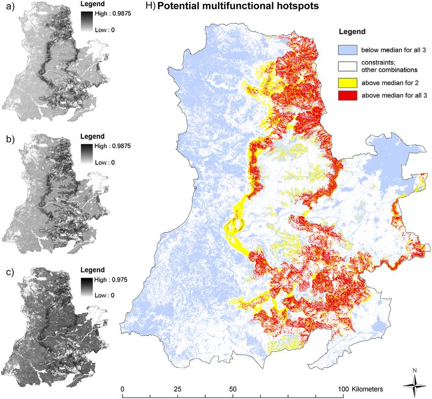
feasibility, respectively. restoration areas are mainly separated within the
Altogether, identified restoration areas extend northern and southern mountain ranges. Whereas
over 50,375 ha, which is about 3.8% of the study larger-scale corridors (north–south) are inter-
area and accounts for about 61% of the forest rupted, connections between existing patches in
cover lost since 1975. Of the overall multifunc- the northern and southern mountain ranges are
tional restoration area, 37,320 ha were identified being enhanced, while simultaneously being
according to multifunctional restoration feasibility relevant for the other two potential functions.
alone, 498 ha for multifunctional regeneration fea- Restoration feasibility alone forms larger con-
sibility alone, and on 12,557 ha multifunctional tinuous patches, whereas regeneration feasibility,
❖ www.esajournals.org 14 January 2017 ❖ Volume 8(1) ❖ Article e01644€
SCHULZ AND SCHRODER
Fig. 6. Value distributions from cross-maps concerning (a) restoration feasibility with multiple functions
(Frest 9 M) and (b) regeneration potential with multiple functions (Freg 9 M). Black lines (dashed and continu-
ous) indicate median values, above which high scoring values for both parameters in (a) and (b), respectively,
were selected as final designated restoration areas.
mostly overlapping restoration feasibility, is more innovative combination of existing tools and meth-
scattered, has a higher prevalence in the southern ods. Several uncertainties and simplifications
mountain range, and is generally localized on underlie large-scale modeling and landscape
higher elevations. restoration planning, largely influenced by limited
data availability, uncertainties regarding the data
Evaluation of designated restoration areas quality, and underlying modeling assumptions
Restoration areas overlap with current land (Holl et al. 2003). Despite several simplifications,
cover types (2008) as shown in Table 2. Most des- this study can be considered a first attempt
ignated restoration areas are on current shrubland, towards a restoration planning approach, includ-
altogether on 43,194 ha (85.7%), followed by ing several targets generally aimed for in the con-
bareland with 6439 ha (12.8%), pastures with text of Forest Landscape Restoration, which have
6333 ha (1.3%), and agriculture on 108 ha (0.2%). so far been little explored in an integrative manner.
Of all designated restoration areas, 55.1% were
deforested within the period 1975–2008, while Restoration suitability and regeneration potential
44.9% have been without forest cover since 1975, based on historical patterns
mainly consisting of shrublands (18,1657 ha). By using empirical data on recent historical
forest occurrence and regeneration and formally
DISCUSSION assessing them in relation to biophysical and
socio-economic factors while accounting for
Landscape-scale restoration programs need to
consider the integration of approaches to achieve Table 2. Extent of current land cover types, deforested
multiple goals (Hobbs 2002). Using an approach land after 1975, and land without forest cover since
combining recent historical forest patterns and 1975 within designated restoration areas.
multiple functions, we have been able to identify Restoration Regeneration Sum
restoration areas that potentially achieve functional Land cover (ha) (ha) (ha)
synergies, while distinguishing between areas suit- Shrubland 32,049.4 11,145.0 43,194.3
able for restoration and areas where natural regen- Bareland 4595.2 1843.7 6439.0
eration could be fostered. These results support Pasture 571.1 61.7 632.8
that traditional approaches, such as the selection of Agriculture 104.4 3.7 108.1
restoration areas based on historical references, can Streams 0.4 0.5 0.8
be combined with targets to enhance multiple Total area 37,320.4 13,054.6 50,375.0
Deforested after 1975 21,085.6 6680.4 27,766.0
functions on a landscape scale using an integrated
No-forest since 1975 16,234.8 6374.2 22,609.0
planning approach. We achieved this through an
❖ www.esajournals.org 15 January 2017 ❖ Volume 8(1) ❖ Article e01644You can also read