WP 1 PRONA Responsibility for Deliverable
←
→
Page content transcription
If your browser does not render page correctly, please read the page content below
D.T1.5.2 Applying remote sensing techniques to identify and monitor forest
disturbances

WP 1 PRONA

Responsibility for Deliverable
Christian Ginzler (WSL)

Contributors
Marc Adams (BFW), Anne Hormes (BFW), Veronika Lechner (BFW)
Innsbruck, December 2019

D.T1.5.2 – Applying remote sensing techniques                          1
GreenRisk4Alps Partnership
BFW           Austrian Forest Research Center (AT)
DISAFA        Department of Agricultural, Forest and Food Sciences, University of Turin (ITA)
EURAC         European Academy of Bozen-Bolzano – EURAC Research (ITA)
INRAE         French national research institute for agriculture, food and the environment,
              Grenoble regional centre (FRA)
LWF           Bavarian State Institute of Forestry (GER)
MFM           Forestry company Franz-Mayr-Melnhof-Saurau (AT)
SFM           Safe Mountain Foundation (ITA)
UL            University of Ljubljana, Biotechnical Faculty, Department of Forestry and
              Renewable Resources (SLO)
UGOE          University of Göttingen, Department of Forest and Nature Conservation Policy
              (GER)
WSL           Swiss Federal Institute for Forest, Snow and Landscape Research (CH)
WLV           Austrian Service for Torrent and Avalanche Control (AT)
SFS           Slovenia Forest Service (SLO)

D.T1.5.2 – Applying remote sensing techniques                                                   2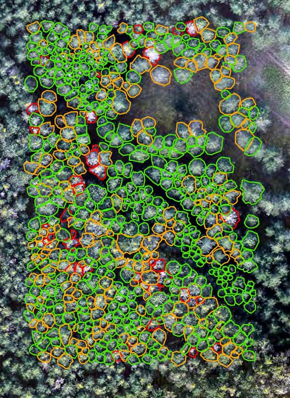
Contents

Abbreviations                                                                      4
Figures                                                                            5
Tables                                                                             7
Introduction                                                                       8
Overview of EO-techniques                                                      10
  Satellites                                                                   10
  Unmanned Aerial Systems                                                      11
Case Studies                                                                   13
  Rapid assessment of Storm Damages with Sentinel-1AB                          13
    Introduction                                                               13
    Study areas and data                                                       15
    Results                                                                    17
    Presentation and dissemination of results                                  17
  Analysis of drought effects after the dry/hot summer 2018                    18
    Introduction                                                               18
    Remote sensing data                                                        19
    Mapping drought stress on forests                                          19
    Mapping forest disturbances in 2019                                        20
    Additional datasets                                                        21
    Results                                                                    24
                Drought stress on forests                                      24
                Forest disturbances in 2019                                    27
                Link between drought stress in 2018 and disturbances in 2019   29
    Discussion and conclusion                                                  30
  Fungal infestation of Pinus nigra in Lower Austria with UAS                  32
    Background                                                                 32
    UAS campaign                                                               34
  Monitoring a forest fire area in Tyrol (UAS)                                 38

D.T1.5.2 – Applying remote sensing techniques                                  3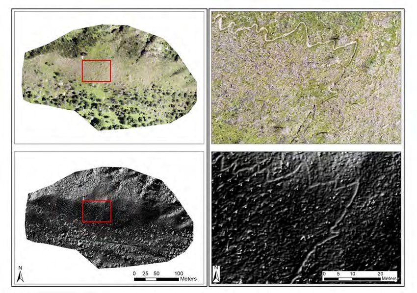
Satellite platforms for forest monitoring and hazard mapping                   46
Appendix                                                                       54
References                                                                     56

Abbreviations

AdTLR          Office of the Tyrolean Regional Government
CIR            Colour Infrared
EO             Earth Observation
InSAR          Interferometric synthetic aperture radar
LiDAR          Light Detection and Ranging
RGB            Red Green Blue
SAR            Synthethic aperture radar
S1/S2          Sentinel 1 / 2
UAS            Unmanned Aerial Systems (aircraft including controlling unit)
WLV            Austrian Service for Torrent and Avalanche Control

D.T1.5.2 – Applying remote sensing techniques                                  4
Figures
Figure 1: Frequency map for the minimum number of SAR images of Sentinel-1. ........................ 14
Figure 2: Localisation of the various storm damage cases processed .......................................... 15
Figure 3: Representation of the coordinate pairs of indications for storm damage with a minimum
area of 0.5 ha. On the left, a general overview of Switzerland after "Burglind", on the right, a
greatly enlarged section near Kestenholz (SO). The interactive result for the whole of
Switzerland can be accessed at https://tinyurl.com/Hinweis-Cluster. © Open street map. 18
Figure 4: Study area (left) and Sentinel-2 tiles covering Switzerland (right) .................................. 19
Figure 5: Example of the forest mask (right) used in this study around the city of Schaffhausen.
Areas of forest not covered by the mask (top right, left bottom) are outside the study region.
.............................................................................................................................................. 22
Figure 6: Example of the forest mixture dataset used for this study around the city of Schaffhausen.
Darker green colors represent pure needleleaf forest areas, light green needleleaf-
dominated, light red deciduous-dominated and dark red pure deciduous forest areas. ..... 23
Figure 7: Spatial distribution (in red) of Picea abies (left) and Fagus sylvatica (right) around the area
of Schaffhausen. Notice that since these data represent the potential spatial distribution of
the species they are not mutually exclusive. Thus, a significant spatial overlap can be
observed. .............................................................................................................................. 23
Figure 8: Example of the vegetation height dataset used for this study around the city of
Schaffhausen. Green colors indicate trees with a height between 3-15m, blue trees with a
height between 15-25m and red color trees higher than 25m. ........................................... 24
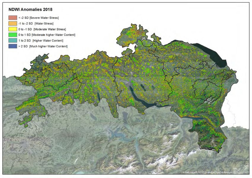
Figure 9: NDWI anomalies for 2018 for the extent of the study region. ........................................ 25
Figure 10: Percent of total forest area under severe water stress per canton within the study region.
The numbers on top of the bars represent the actual forest area in ha (based on the NFI
forest mask) under severe water stress. .............................................................................. 26
Figure 11: Percent of forest species potentially present at the areas under severe water stress in
2018. .................................................................................................................................... 27
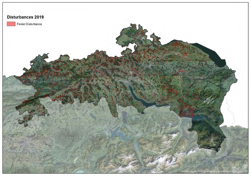
Figure 12: Forest disturbances in 2019 for the extent of the study region. .................................. 28
Figure 13: Percent of forest disturbances relative to the total forest area per canton within the study
region. The numbers on top of the bars represent the actual forest area of disturbances in
ha. ......................................................................................................................................... 29
Figure 14: Relationship between forest areas where disturbances were detected in 2019 and their
respective NDWI anomalies in 2018. For clarity, NDWI anomalies of 2018 are reclassified to
four classes........................................................................................................................... 30
Figure 15 Black pine stands near Steinfeld showing different degrees of Diplodia sapinea
infestation. ............................................................................................................................ 33
D.T1.5.2 – Applying remote sensing techniques 5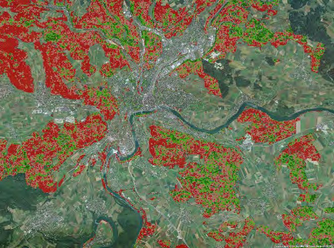
Figure 16 Multiplex Mentor UAS (left); daylight (Sony NEX5) and multispectral (Mica Sense RedEdge
3) cameras used on-board the Mentor, with corresponding spectral range (sources:
MicaSense, dpreview.com, BFW).......................................................................................... 35
Figure 17 UAS-OP of the study site; overview (left) and detail (right). ............................................ 36
Figure 18 Comparison of RGB (left) and NDVI (right) imagery over infected Pinus nigra crowns
(circled in blue). .................................................................................................................... 36
Figure 19 Subplot of Pinus nigra crowns classified into healthy (green), infected (orange) and dead
(red) classes. ........................................................................................................................ 37
Figure 20 Distribution of NDVI-values within tree classes 1-3 (left) and relative frequency of trees
classified as healthy, infected and dead within the same classes....................................... 37
Figure 21 Overview of lower burnt section at the Hochmahdkopf on 24 April 2014 (left); damaged
avalanche defense structures and charred mountain pine in the upper burnt section on 10
April 2014 (right). ................................................................................................................. 39
Figure 22 Results of the data collection on 4 July 2017 - orthophoto (top) in overview (left) and
detail (right) (GSD: 0.05 m), Relief of the DSM (bottom) in overview (left) and detail (right)
(GSD: 0.2 m); the red polygon indicates the enlarged area. ................................................ 40
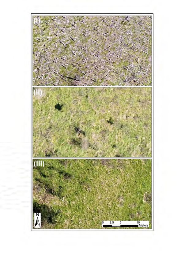
Figure 23 Comparison of the shares of the erosion classes in 2015 and 2017 (left); examples of
the erosion classes based on the orthophoto 2017 (I - high, II - medium, III - low) (right). .. 42
Figure 24 Height difference of the DSMs from 2014-2017 (left column) for the erosion intensities
(top) and vegetation classes (bottom) (N = 12,891); examples of vegetation classes a) -
vegetation-free soil (I), b) - sparse grass vegetation (II), c) - area-wide grass/herb vegetation
(III) from the 2017 orthophoto (right column); the newly constructed glide snow frames are
visible as triangular features in (I). ....................................................................................... 43
Figure 25 Detailed view of orthophotos from the lower burnt area of the Hochmahdkopf in 2014
(left) and 2017 (right), illustrating the rapid successional development in severely burnt
areas. .................................................................................................................................... 44
D.T1.5.2 – Applying remote sensing techniques 6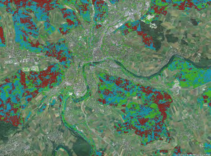
Tables
Table 1: List of the area distribution of the reference area damage (ha). ..................................... 16
Table 2: SAR backscatter behavior for the two polarizations VV and VH of all four areas. ............ 16
Table 3 Overview of satellite products for forest monitoring such as tree cover, storm damages and
      drought effects ..................................................................................................................... 49
Table 4 Overview of satellite products useful for the exploration of natural hazards .................... 49
Table 5 Data hubs to access satellite imagery for various applications ........................................ 47
Table 6 Satellite data access points for remote sensing specialists ............................................. 52
Table 7: Technical specifications of the Mentor UAS (Adams et al., 2016) ................................... 54
Table 8: Properties of UAS-flights on 15 November 2015. ............................................................ 55

D.T1.5.2 – Applying remote sensing techniques                                                                                           7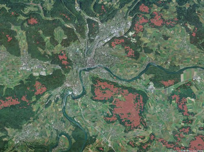
Introduction

Remote sensing in the forest has a very long tradition. The view from above facilitates orientation
and allows views that would never be possible from the ground. Dividing the forest into stands or
treatment units would be much more difficult and time-consuming without e.g. aerial photography
- in some cases not possible at all. Detailed interpretation keys have been and are being used to
try to make the interpretation consistent and reproducible. The increasing availability of digital data
and products from remote sensing has paved the way for automated procedures. A great deal is
already operational. For example, in addition to digital orthophotos, which are common tools in the
age of Google Earth or Bing Maps, digital 3D vegetation elevation models are also available to
visualize stand heights and forest structures, to use them as a basis for planning or to derive 3D
features over large areas and longer time periods.
However, the data already available today make much more possible. Many forest functions can
be quantified using remote sensing methods. Wood supply as a resource can be measured to a
large extent by height, biodiversity by the vertical and horizontal forest structure and protection by
crown density, distribution of trunks and tree species. Some features cannot be measured directly,
but indirect models must be applied.
Data from satellites are very easily available today, but since several years data hosts and remote
processing options have been popping up and it might be difficult to keep track of which resources
and processing servers might be best for various user needs. We therefore give a brief overview
for three different types of users (forest, natural hazard and remote sensing specialists) and where
satellite data are accessible. The spatial resolutions are comparable to those of aerial photographs.
Satellite images are available today with sub-meter ground resolution. Besides the ever-increasing
spatial resolution of satellite data, the temporal resolution is also improving. The opening of image
archives and the free and very easy access to satellite data (e.g. Landsat archive, Sentinel) has
stimulated research and development work. Such time series, e.g. dating back to the 1990s for
Landsat, have great potential for monitoring and analyzing changes, disturbances and
interventions at global and regional level. One example is the "Global Forest Change" project, which
makes changes in forests freely available online with a temporal resolution of one year and a spatial
resolution of 30 m (Hansen et al 2013).
Excellent results of case studies sometimes have to be put into perspective for large area
applications. The intensive exchange between research and practice is indispensable. Today, there
are many possibilities for practical applications to integrate remote sensing into daily work
processes.
In the report on remote sensing methods for the identification and permanent monitoring of forest
disturbances, different sensors on different platforms are discussed. Forest disturbances are
understood as both abrupt changes (e.g. storm, fire, avalanches) and long-term changes (e.g.
changes/damages caused by drought, insect infestation, frost).

D.T1.5.2 – Applying remote sensing techniques                                                      8
The report presents and discusses the potentials and applications of the various platforms. For
small-scale damage, unmanned aerial vehicles (UAVs) are very efficient and flexible platforms. With
simple sensors, such as RGB cameras, data on small-scale events can be captured very quickly.
The benefit of other sensors (CIR, LiDAR, spectrometer) will be discussed. If larger areas are
affected by disturbances, it makes more sense to use helicopters and airplanes. The pro and cons
of cameras (RGBN) and LiDAR are discussed as sensors. For larger areas, data from satellites with
a very high temporal and acceptable spatial resolution are available today. Multispectral data from
Sentinel-2ab (>= 10m x 10m) are available at intervals of 3-5 days. The advantages and
disadvantages of multispectral sensors (intuitively interpretable but no data in cloudy conditions)
are discussed. Alternative methods with RADAR (Sentinel-1ab) are presented.
The different approaches are presented in the case-study chapter. Examples on ongoing work and
recent studies with different platforms and sensors are presented:

   1. Rapid assessment of Storm Damages with Sentinel-1
   2. Analysis of drought effects after the dry/hot summer 2018 with Sentinel-2
   3. Fungal infestation of Pinus nigra in Lower Austria with UAS
   4. Avalanche forest damage in Tyrol with UAS

A last chapter will present an overview of free and paid access and platforms to Earth observation
data useful for forest degradation, disturbances and natural hazard monitoring.

D.T1.5.2 – Applying remote sensing techniques                                                  9
Overview of EO-techniques

Satellites
The accessibility to satellite data for forest and natural hazard monitoring has skyrocketed in the
last decade, not least because the European Space Agency (ESA) has an open access policy. For
monitoring services, we may differentiate optical and radar systems.
Optical Earth Observation data sets that are useful for forest and natural hazard monitoring have
in general a high resolution between 5 and 30 m. Very high resolution (VHR) resolution sensors
have a pixel size of < 2 m and the capacity to give very precise information on forest degradation
or the details of a natural hazard deposit. However, the repeat cycles might either be cost intensive,
as data acquisition might just happen on demand. Medium to coarse resolution sensors with 30 to
> 60 m ground resolution have lower costs and are often open access data still offering the
potential for forest monitoring. Landsat satellites deliver multispectral data since 1972 and are
available without restrictions from the USGS (United States Geological Survey). The new generation
of Landsat 7 and 8 are available on e.g. the Google Earth Engine without restrictions. ESA follows
also a strict open access policy for the optical multispectral Sentinel-2 satellites and the Synthetic
Aperture Radar (SAR) satellites Sentinel-1A/B.
Optical satellites cover wavelengths between 400 and 13000 nm and are given in detail in Tables
3-6. Satellite data are processed with image processing methods and thus valuable products for
forest monitoring are gained (Hirschmugl et al. 2017). Different indices can be used for forest
change monitoring: normalized difference vegetation index (NDVI), enhanced vegetation index
(EVI), normalized burnt rate (NBR), and the soil-adjusted vegetation index (SAVI) (Hirschmugl et al.
2017). Changes in forest crown cover are mapped based on mapping methods developed over the
last 10 years (Banskota et al. 2014, Hansen et al. 2014).
Radar satellite data are available since the 90ies, but with the recent launch of Sentinel-1A/B
satellites in 2014 and 2016 with a repeat cycle of only 6 days, the potential to use Synthetic
Aperture Radar (SAR) offers a very high potential to use radar data for forestry applications
(Kellndorfer 2019, Siqueria 2019). The SAR-principle is based on actively transmitting
electromagnetic microwaves and analyzing its echo. SAR has the advantage that it provides data
during the night, even when it is cloudy, though it is not completely weather insensitive and
atmospheric signals and terrain have to be considered. SAR platforms deliver data with high spatial
resolution between
SAR datasets have been used to Monitoring, Reporting and Verification (MRV) in various countries
and the combination of different platforms with different bands (X, C or L-band) offer yet to explore
options such as capturing forest stand heights, canopy characterization biomass and forest
structure (Flores-Anderson et al. 2019, Dostálová et al. 2016). Major challenges of the SAR method
are data storage and processing capacities and the lack of consistent workflows to process data
not just for pilot regions.

Unmanned Aerial Systems
Advances in recent years in the fields of aircraft construction (light weight construction & engine
development), navigation (GNSS – Global Navigation Satellite System & IMU – Inertial
Measurement Unit) as well as mechatronics in general (mechanics, electrical engineering &
informatics) and digital photogrammetric software design in particular, have given rise to the
development of Unmanned Aerial Systems (UAS) (Briese et al., 2013). The term UAS is used here
according to the recommendation by the International Civil Aviation Organization; other
denominations include Unmanned Aerial Vehicle (UAV), Remotely Piloted Aircraft System (RPAS) or
drone. UAS is the collective designation for an aircraft and its associated elements which are
operated with no pilot on board (ICAO, 2020). According to the classification suggested by Watts et
al. (2012), the type of aircraft may range from Micro or Nano Air Vehicles (MAV/NAV) with a typical
flight time of 5-30 min, operating at very low altitudes (< 330 m), to High Altitude, Long Endurance
(HALE) platforms, operating at altitudes of 20,000 m and more and with flight times of > 30 h, used
for both civil and military missions. In the context of this deliverable, the term UAS refers to the
scientific use of different types of Low Altitude, Short Endurance (LASE) aircraft with a typical weight
of < 5 kg, flight times of 20-40 mins and a wing span of < 3 m, optimized for easy field deployment
/ recovery and transport. The three main platforms available within this definition of UAS include
fixed-wing aircraft, helicopters and multicopters.
In general, UAS are able to bridge the gap between full-scale, manned aerial, and terrestrial, field-
based observations (Briese et al., 2013; Rosnell & Honkavaara, 2012). The primary advantages of
the LASE UAS include the possibility for flexible, cost-effective, on-demand mapping missions with
multiple sensors at an unprecedented level of detail (ground sampling distance (GSD) of few
centimetres or millimetres, depending on camera properties and flight height) (Ryan et al. 2015).
Due to the fact, that UAS are operated at lower altitudes, medium / high level clouds or haze also
less influences them. Due to their small size however, they can only be operated under favourable
weather conditions (e.g. low wind speed, good visibility). From a scientific point-of-view, UAS offer
the advantage of allowing a flexible matching of the required spatial resolution and sensor type to
the specific application, i.e. research question at hand (Colomina and Molina 2014; Lucieer et al.
2014); this is reflected in a wide range of recent reports on UAS-related forestry applications (Tang
& Shao, 2015), which include: Forest surveying (Paneque-Galvez et al., 2014; Koh & Wich, 2012);
canopy gap mapping (Getzin et al., 2012 ); forest wildfire tracking (Lechner et al., 2019b; Ambrosia
et al., 2011; Hinkley & Zajkowski, 2011); forest management (Wang et al., 2014; Felderhof &
Gillieson, 2011). Further applications of UAS include monitoring: soil erosion (e.g. D’Oleire-

D.T1.5.2 – Applying remote sensing techniques                                                      11
Oltmanns et al., 2012), landslide and debris flow (e.g. Niethammer et al., 2012; Sortier et al.,
2013), slope deformations (Hormes et al. 2020), archaeology (e.g. Verhoeven, 2011), seasonal
snow (e.g. Bühler et al., 2016), geomorphology (e.g. Hugenholz et al., 2013) and hydrology (e.g.
Molina et al., 2013). A detailed summary of civil UAS applications is supplied by González-Jorge et
al. (2017).

The development of novel computer vision techniques and their implementation into a wide range
of software packages, have considerably reduced the requirements for the recorded data (Vander
Jagt et al. 2015; Turner et al. 2012). Processing the UAS imagery is therefore usually performed
with off-the-shelf or custom structure-from-motion photogrammetry software; for a comprehensive
review on available software options, see Nex and Remondino (2014) or Colomina and Molina
(2014). Standard outputs are orthophotos, digital surface models (DSM) and (RGB-)coloured 3D
dense point clouds (DPC). DSMs generally refer to the height of the terrain, buildings or vegetation,
captured in the scene (Adams et al. 2016). The DSM is interpolated from DPC, generated with
multiview stereo reconstruction as part of the photogrammetric workflow (Vander Jagt et al., 2015).
When calculating terrain height changes (e.g. when mapping mass movements in forested terrain)
all objects on or above the terrain should be removed. This is typically achieved by classifying the
DPC into ground and non-ground points, and subsequently generating a digital terrain model (DTM).
The use of photogrammetric DTMs may be limited in densely forested areas, as only few ground
points are recorded. Therefore, masking out the process area before calculating terrain height
change may avoid potential errors (Tang & Shao, 2015).

D.T1.5.2 – Applying remote sensing techniques                                                   12
Case Studies

Rapid assessment of Storm Damages with Sentinel-1AB

This study was conducted by Marius Rüetschi, Lars Waser, David Small and Christian Ginzler as a
collaboration between the Federal Office for the Environment (FOEN) and the Swiss Federal
Institute for Forest, Snow and Landscape Research WSL (Rueetschi et al. 2019).

Introduction
After a major storm event, it is of interest to quickly gain an initial overview of the damage caused
to the forest. Satellite-based remote sensing is ideally suited for this purpose, as it can provide such
an initial overview after a short time, at relatively low cost and for a large area (e.g. the whole of
Switzerland). Studies show that satellites with optical sensors are well suited for this. Damage can
be located with a high degree of accuracy (Baumann et al., 2014; Einzmann et al., 2017). This has
also been shown specifically for Switzerland in a project on forest monitoring with sentinel 2
satellite images financed by the Federal Office for the Environment (FOEN) (Weber and Rosset,
2019). Optical sensors have the disadvantage, however, that it is not possible to record the earth's
surface when it is cloudy. Therefore, a guaranteed and rapid data availability after a storm event is
not given. Since most large-scale storm events in Switzerland occur in the autumn and winter
months (Usbeck, 2015), when the probability of cloudiness is high, the availability of evaluable
satellite images shortly after the event cannot be guaranteed. Therefore, it was investigated
whether there are possible alternatives and synergies with Synthetic Aperture Radar (SAR) data,
which record data of the earth's surface independent of cloudiness and therefore have a high
recording frequency. An overview of the frequency of the two SAR satellites Sentinel-1A/B is shown
in Figure 1. The lowest frequency of at least 2 SAR recordings within 6 days occurs in two wedges
over Western Switzerland and Eastern Switzerland. Otherwise, at least 3 SAR images within 6 days
are available for the whole of Switzerland.

D.T1.5.2 – Applying remote sensing techniques                                                      13
Figure 1: Frequency map for the minimum number of SAR images of Sentinel-1.

Based on a thunderstorm in the northern canton of Zurich on 2 August 2017 and the "Xavier"
autumn storm of October 2017 in Mecklenburg-Western Pomerania, a project at the WSL in
cooperation with the University of Zurich developed a method for generating indications of
extensive storm damage in 2018 (Rüetschi et al., 2019). For this purpose, data from the Sentinel-
1 satellite pair, which are equipped with SAR sensors, are used. The method is based on a novel
combination of several individual SAR images developed at the University of Zurich (Small et al.,
2019), which reduces the noise to such an extent that short-term and larger changes in SAR
backscatter in the forest can be perceived as indications of storm damage.
Within the framework of this project, it was investigated whether this method, which was developed
for events in leafy conditions, can also be applied to unleafed conditions in winter. Supraregional
storm damage usually occurs in winter with unsuitable conditions for satellite or aerial photography
with optical sensors (Usbeck, 2015). Prominent examples are the storms "Vivian" in 1990, "Lothar"
in 1999 and "Burglind" in 2018, making a potential application of the method with SAR data all the
more promising. However, since factors such as snow and temperatures below freezing point have
a strong influence on SAR backscatter in winter, their influence on a successful application was
investigated within the scope of this project.
Data from the most recent major storm events in Switzerland were collected. Subsequently, the
following possible influencing factors on SAR backscatter in different study areas (depending on
the availability of corresponding reference data) were analyzed in order to explore possible further
development potential of the method:
    -   Temperature
    -   Precipitation
    -   Lying snow
    -   Water content in snow
    -   Vegetation height
    -   Crown coverage
    -   Degree of forest mixture
    -   Slope
    -   Aspect

D.T1.5.2 – Applying remote sensing techniques                                                  14
On the basis of these findings, the method of Rüetschi et al (2019) was then further developed. The accuracy achieved with the revised method in the detection of windthrows is shown. The accuracy is shown as a function of the number of SAR images (= time required after a storm) and of the minimum size of the damage areas to be detected. In addition, the values of the newly developed area proxy are briefly discussed. Different ways to publish the data to potential stakeholders are shown. Study areas and data In order to cover as many different storm events as possible, mapped references from various storm damage cases in Switzerland were collected. The references come from different times of the year and range from topographically flat (e.g. Central Plateau) to complex areas (e.g. Alps). Storm damage references could be obtained from the following areas and storms: Figure 2: Localization of the various storm damage cases processed Since at least 5 SAR images were available for all of the study areas before and after the storm event, the entire analyses were subsequently performed on 5 SAR images for comparison with Local Resolution Weighting (LRW) composites. The LRW composites were calculated in two phases by David Small at the University of Zurich (UZH) using a UZH algorithm. In a first phase, the individual SAR images were corrected both geometrically and radiometrically using a digital elevation model (Federal Office of Topography Swisstopo, 2018) (Small, 2011). In a second phase, in order to reduce the noise typical in individual SAR images, two LRW composites were calculated from these 5 SAR images for before and after the respective storm event (Small et al., 2019). Reference data were available on the basis of terrestrial mapping or the interpretation of high-resolution remote sensing data ( Table 1). D.T1.5.2 – Applying remote sensing techniques 15
Table 1: List of the area distribution of the reference area damage (ha).

 Event                Date           Area        0-0.5   0.5-     1-       1.5-    2-2.5       2.5-3     >3         Total      Type
                                                         1        1.5      2                                                   of ref.
 Thunderstorm         02.08.17        TG         38       12          4     2      5           2         1          64         Field
 Burglind             04.01.18        EN         17       21          8     4      3           0         2          55         Planet
 Burglind             04.01.18        SO         6        12          2     4      0           3         8          35         Field
 Vaia                 30.10.18        VABE       47       6           2     0      1           0         2          58         Planet
 Total                                           122      55          16    12     10          5         14         234

If we look at the differences in SAR backscatter δ between the forest and the windthrows references
of the different areas, we see that the same effect can be observed in all areas, on which the
method is based. The δ values for windthrows are generally higher than for forest (Table 2, second
last column). The fact that the δ values from the forest are also positive for all areas may be
because the damage areas are all included in the class 'forest'. In addition, there are also
potentially unmapped damages in each area.
Likewise, the variance of the SAR backscattering difference δ is larger within the windthrows areas
(Table 2, last column). Another interesting observation regarding the variance (or standard
deviation) is the lowest standard deviation in the area with the flattest topography (DE). The more
complex the area, the higher the standard deviation. From this, it can be concluded that an
extraction of wind casts based on the differences in the SAR backscatter difference δ is more
difficult and less accurate in topographically more complex areas. Within the scope of this project,
therefore, an attempt was made to find explanations for the observed differences.

Table 2: SAR backscatter behavior for the two polarizations VV and VH of all four areas.

 Area       Pol.             Forest area                              Windthrows                              Difference

                      mn δ         sd δ                       mn δ          sd δ                       mn δ diff            sd δ diff
                                                     n                                     n
                      [dB]         [dB]                       [dB]          [dB]                           [dB]                 [dB]

  SO        VV         0.3        1.35       71751            0.87          1.38    8963                     0.57              0.03
  SO        VH        0.33        1.33       71751            0.86          1.38    8963                     0.53              0.05
  TG        VV        0.05        1.58       80354              0.5         1.78    4101                     0.45                0.2
  TG        VH        0.31         1.6       80354            0.97          1.81    4101                     0.66              0.21
  EN        VV        0.24        1.87      1135451             0.4         1.93    4104                     0.16              0.06

D.T1.5.2 – Applying remote sensing techniques                                                                                    16
EN VH 0.42 1.97 1135451 0.58 1.96 4104 0.16 -0.01
VABE VV 0.31 1.62 18492 0.45 1.68 3070 0.14 0.06
VABE VH 0.32 1.62 18492 0.3 1.7 3070 -0.02 0.08
Results
Three factors had a decisive influence on the quality of the method: the height of vegetation, the
content of liquid water within the snow cover and the topography.
- Only from a vegetation height of 15 m reliable differences in radar backscatter between
intact forest and windthrows can be detected. Thus, relevant stands can be covered.
- Liquid water within the lying snow cover influences the radar backscattering so strongly that
it makes the application of the method in areas with wet snow impossible.
- Radar sensors do not reliably measure the backscatter in areas with steep slopes (> 60°)
for reasons of recording geometry. This corresponds to a forest area of approx. 5% in
Switzerland as a whole.
The method was developed on the basis of these findings. Indications for storm damage in stocked
areas of 15 m and above are shown. In the "Burglind" case, large parts of the foothills of the Alps
were affected by wet snow, so these areas were excluded from the evaluation. In the future, this
influence should be specifically investigated in order to make appropriate adjustments to the
method, so that indications of storm damage can also be generated in these areas. The 5% of
forest areas from which no reliable radar measurements can be made were also excluded from the
procedure.
Presentation and dissemination of results
The result of the procedure is a reference card for storm damage. In order not to suggest an exact
mapping with the result, the clues are presented in generalized form as a grid of hectares or as
point clues in the form of coordinate pairs. Figure 3 shows an example for the representation of the
point clue. An automatic cluster algorithm adapts the representation of the points according to the
selected room section.
D.T1.5.2 – Applying remote sensing techniques 17Figure 3: Representation of the coordinate pairs of indications for storm damage with a minimum area of 0.5 ha. On the left, a general overview of Switzerland after "Burglind", on the right, a greatly enlarged section near Kestenholz (SO). The interactive result for the whole of Switzerland can be accessed at https://tinyurl.com/Hinweis-Cluster. © Open street map. Analysis of drought effects after the dry/hot summer 2018 This study was conducted by Achilleas Psomas and Charlotte Steinmeier as a collaboration between the Federal Office for the Environment (FOEN) and the Swiss Federal Institute for Forest, Snow and Landscape Research WSL (Psomas et al. 2019). Introduction In 2018, Central and Northern Europe – including Switzerland – experienced one of this region's most severe droughts of the last century which in some areas was worse than the drought of 2003 (Buras et al. 2019). In Switzerland the spring and summer months of 2018 were characterized by a unique combination of low precipitation and high temperatures which had a significant effect on water supplies of lakes and rivers, glacier melting and increased forest fires hazard. In particular, 2018 summer temperature differences were 3.5 °C higher and precipitation 40% lower compared to the long term average (Brun et al. 2020). The effects of the drought were especially severe in the north-eastern part of Switzerland (Brunner et al. 2019) and on forests ecosystems in these areas. Large areas of forest showed premature canopy browning with species like Fagus sylvatica and Picea abies (amongst others) showing signs of stress as a response to the drought. While a number of studies exist that analyse the drought of 2018 (Pestalozzi 2019) its direct impacts on forest ecosystems of Switzerland and their subsequent effects in 2019 are still unexplored. In this study we wanted to explore the potential of remote sensing and in particular of ESA’s Sentinel-2 mission to a.) map the areas of forest under drought stress in 2018 for the north-eastern part of Switzerland and investigate which forest mixture groups (deciduous-needleleaf gradient), tree species and tree ages groups were affected the most. We also aimed at b.) investigating the potential effects of the 2018 drought in forest areas in 2019 by using remote sensing to detect and map forest disturbances in 2019. How much of these could be attributed/linked to the drought D.T1.5.2 – Applying remote sensing techniques 18
of 2018? This work was performed at the scale of the whole north-eastern part of Switzerland but
also at the scale of Cantons (Figure 4).
Remote sensing data
The remote sensing data used for this study were optical Sentinel-2 MSI (Drusch et al. 2012) covering the whole extent
of the study region. Sentinel-2 is a wide-swath, high-resolution, multi-spectral imaging mission by ESA for monitoring
vegetation cover, soil and water cover. Sentinel-2 Level-1C and Level-2A data were used. Level-1C data are radiometric
and geometric corrected Top-Of-Atmosphere products and Level-2A are Surface Reflectance data. The corrections
include orthorectification and spatial registration on a global reference system (combined UTM projection and WGS84
ellipsoid) with sub-pixel accuracy. Sentinel-2 data are delivered in tiles of 100×100 km. From the eleven tiles covering
the extent of Switzerland (

Figure 4), four were required to cover the study region (32TLT, 32TMT, 32TNT, 32TNS).

Figure 4: Study area (left) and Sentinel-2 tiles covering Switzerland (right)

Initial analyses included removing cloud-contaminated pixels. Upon investigation of the early
results, we realized that the cloud mask provided by ESA did not sufficiently remove all cloud pixels.
We thus decided to continue the analyses with Sentinel-2 tiles that had cloud coverage of 50% and
below. All analyses were performed on the Google Earth Engine (GEE) (Gorelick et al. 2017). GEE
is a cloud-based geospatial-processing platform for executing large-scale spatial data analysis with
multi-petabyte catalog of satellite imagery, climate, demographic, and other global or regional
vector datasets available.

Mapping drought stress on forests
To map drought stress on forests we used Sentinel-2 Level-1C data to calculate the Normalized
Difference Water Index (NDWI) (Gao 1996) for the extent of the study region. NDWI is an index
derived as the normalized difference between the Near-Infrared (NIR) and Short Wave Infrared
(SWIR) channels of the electromagnetic spectrum. The potential of NDWI as a proxy of vegetation
water content and its usefulness for drought monitoring has been shown in literature (Liu et al.
2004, Gu et al. 2008). The reflectance of the SWIR channel is linked to changes in the vegetation

D.T1.5.2 – Applying remote sensing techniques                                                                     19
water content and the mesophyll structure of vegetation canopies. The NIR reflectance is
determined by leaf internal structure and leaf dry matter content but not by water content. By
combining the NIR with the SWIR channels spectral differences due to leaf internal structure and
leaf dry matter content are minimized, and we thus improve the accuracy in the retrieval of
vegetation water content
In this study we calculated the anomalies of NDWI for 2018 in comparison to a base period of
normality defined as years 2016-2017. In particular we calculated NDWI anomalies for the
reference period between July 20th (DOY: 201) and August 31st (DOY: 243) when the drought had
reached its most severe period and the effects of it started being even visually visible on forests.
While Sentinel-2 data exist since 2015 only years 2016-2017 were used as a base/normality
period to 2018. Year 2015 was intentionally excluded due to very warm and dry conditions that
also led to a drought across large parts of Europe and Switzerland (Ionita et al. 2017).
A total of 73 (2016-2017) and 62 (2018) Sentinel-2 tiles were considered for the analyses. For
each tile, the NDWI was calculated at 10m resolution using the NIR (Band 8) and SWIR (Band 11)
of the Sentinel-2 sensor. Then for the reference period of 2016-2017 and for 2018 the median
was calculated using all the available data for the respective years. Using the median was a better
representation of the true value of the pixel compared to the mean since data might still
contaminated with rather high or low values like remaining clouds and their shadows. Finally, the
NDWI anomalies for 2018 were as shown in Equation 1.

The NDWI anomalies were calculated in standard deviation units that ranged typically from -4 to
+4. Negative values represented areas with lower vegetation water content in comparison to the
reference period. Values between -1 to +1 were considered normal while values larger than 1 or
lower than -1 higher/lower than normal.

Mapping forest disturbances in 2019
In order to investigate the potential effects of the 2018 drought on forest areas, we established a
two-step analysis. First we identified all forest areas that were healthy in 2018. Then we compared
which of these areas had transitioned from a healthy to a non-healthy status in 2019 and finally
examined what the water stress status (NDWI anomaly) of these was in 2018.
To establish healthy forest areas in 2018 we collected all available Sentinel-2 Level-2A data for the
period between April 15th (DOY: 105) and June 30th (DOY: 181). We selected this period to avoid
any significant effects that the prolonged drought could have on the trees, as we could observe
later in 2018. A total of 54 Sentinel-2 tiles were used to calculate the median Normalized Difference
Vegetation Index (NDVI) (Broge and Leblanc 2001) at 10m resolution using the Red (Band 4) and

D.T1.5.2 – Applying remote sensing techniques                                                   20
NIR (Band 8) bands of the Sentinel-2 sensor. All forest areas with an median NDVI value higher
than 0.4 during the period April 15th-June 30th 2018 were considered healthy (Jensen 2007).
We defined forest areas that transitioned from a healthy to a non-healthy status in 2019 as area
where large disturbances (forest timber logging and/or forest mortality) took place between 2018-
2019. To identify these types of disturbances we collected all available Sentinel-2 Level-2A data
for the period between April 15th (DOY: 105) and June 15th (DOY: 166) for 2018 and 2019
respectively. We selected this period, which is rather early in the season, since we realized that in
many areas where forest was removed in 2019 the effect of the newly growing herb/bushy
vegetation had a significant effect on the remote sensing signal. In particular, the more we
progressed into the growing season the accumulating biomass of herbs/bushes led to a spectral
signal which resembled that of a forest. Thus we restricted the period to mid of June (DOY: 166)
A total of 50 (2018) and 22 (2019) Sentinel-2 Level-2A tiles (with cloud coverage less than 50%)
were used to calculate the Normalized Burn Ratio Index (NBR) (Key and Benson 2006) at 10m
spatial resolution using the NIR (Band 8) and SWIR (B12) of the Sentinel-2 sensor. We selected
NBR versus NDVI or any other index since previous research (Cohen et al. 2010, Shimizu et al.
2017) has indicated that NBR is more sensitive in disturbance detection. We used very high-
resolution satellite imagery to visually identify forest disturbances across the whole extent of the
study region. Images were obtained from the PLANET sensor constellation (www.planet.com) at 3-
5m spatial resolution, which allowed for the comparison between 2018 and 2019. After visual
inspections of forest disturbance areas we decided that a reduction larger than 50% on the value
of the value of NBR in 2019 relative to that of 2018 was a good indicator of forest timber logging
and/or forest mortality in our study region.
As a final step we identified which forest areas were healthy in 2018 and at the same time had
deviation of NBR larger than the established threshold between 2018-2019 and used these areas
for further analyses. To ensure reliability of the results only pixels that had at least three Sentinel-
2 observations during each of the given periods in 2018 and 2019 were considered for further
analyses.
Additional datasets
All analyses in this report were restricted to forest areas across the study region. Available forest
mask data from the National Forest Inventory (NFI) at 1m spatial resolution (Waser et al. 2015)
were aggregated to 10m to match the resolution of the Sentinel-2 data. An example of the forest
mask dataset is given in Figure 5.

D.T1.5.2 – Applying remote sensing techniques                                                      21
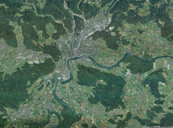
Figure 5: Example of the forest mask (right) used in this study around the city of Schaffhausen. Areas of forest not
covered by the mask (top right, left bottom) are outside the study region.

Since we wanted to investigate which forest mixture groups (deciduous-needleleaf gradient) and
forest species were a.) under drought stress in 2018 and b.) the 2019 disturbances took place, we
used two additional datasets. The first one was the countrywide mapping NFI dataset of
broadleaved and coniferous trees in Switzerland (Waser et al. 2017). In particular, it provided
information about the proportion of deciduous trees at the scale of 25m pixels. Its values range
from 0-100% where 0 indicates 25m pixels where 0% is covered by deciduous and 100% by
needleleaf forest species and 100 indicates that 100% of the pixel is covered by deciduous species.
First, this dataset was resampled to 10m to match the resolution of the Sentinel-2 data. Then, we
reclassified it into four new classes. Pure needleleaf pixels (0-10% proportion deciduous),
needleleaf-dominated (10-50% proportion deciduous), deciduous-dominated (50-90% deciduous
proportion) and pure deciduous pixels (90-100% proportion deciduous). An example of the dataset
is given in Figure 6.

D.T1.5.2 – Applying remote sensing techniques                                                                 22
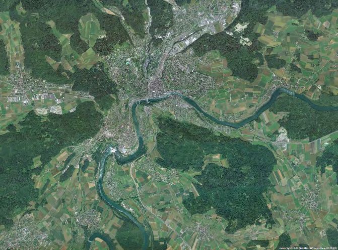
Figure 6: Example of the forest mixture dataset used for this study around the city of Schaffhausen. Darker green colors
represent pure needleleaf forest areas, light green needleleaf-dominated, light red deciduous-dominated and dark red
pure deciduous forest areas.

We furthermore wanted to investigate which forest species were affected by the drought of 2018
and disturbances were detected in 2019. Currently there is no available wall-to-wall dataset at the
species level for Switzerland that is based on actual observations. Thus, we used a dataset (Wüest
et al. 2020) where spatial distribution of forest species were modeled using species distribution
models (SDMs) (Guisan and Zimmermann 2000). These maps represented the potential
distribution of forest species, meaning they showed where a species could theoretically exist
without taking into account factors like competition from other species or human management. For
this work, we selected a set of deciduous and needleleaf forest species whose modeling accuracy
was high (True Skill Statistic > 0.75) and were abundant in the study region, namely: Acer
campestris Acer platanoides, Fagus sylvatica, Fraxinus excelsior, Picea abies, Pinus sylvestris,
Quercus petraea and Quercus robur. An example of this dataset is given in Figure 7.

Figure 7: Spatial distribution (in red) of Picea abies (left) and Fagus sylvatica (right) around the area of Schaffhausen.
Notice that since these data represent the potential spatial distribution of the species they are not mutually exclusive.
Thus, a significant spatial overlap can be observed.

D.T1.5.2 – Applying remote sensing techniques                                                                       23
Finally, to investigate if trees of certain age were more prone to drought stress and forest
disturbances we used the vegetation height model (VHM) dataset from the NFI, available at 1 m for
the extent of the study region (Ginzler and Hobi 2015). Trees with a height between 3-15 m were
considered young in age, trees between 15-25 m adult and trees with height above 25 m
mature/old. The VHM was first aggregated to 10m in order to match the resolution of the Sentinel-
2 remote sensing data and then was reclassified to the three classes mentioned above. An example
of the VHM dataset is given in Figure 8.

Figure 8: Example of the vegetation height dataset used for this study around the city of Schaffhausen. Green colors
indicate trees with a height between 3-15 m, blue trees with a height between 15-25m and red color trees higher than
25m.

Results
Drought stress on forests
The yearly NDWI anomalies for 2018 for the extent of the study region are shown in Figure 9. Areas
that had NDWI difference to the base/normality period (2016-2017) lower than 2 standard
deviations are depicted in red and are considered to be under severe water stress.

D.T1.5.2 – Applying remote sensing techniques                                                                 24
Figure 9: NDWI anomalies for 2018 for the extent of the study region.

Looking at the map we can observe that even at this coarse scale large forest areas in the regions
of Schaffhausen, northern Aargau and Walensee (amongst others) are under severe water stress.
For the remaining of this document we will report only forest areas that were under severe water
stress (NDWI anomalies
Figure 10: Percent of total forest area under severe water stress per canton within the study region. The numbers on top
of the bars represent the actual forest area in ha (based on the NFI forest mask) under severe water stress.

Results showing which forest species were potentially affected by the drought of 2018 are
displayed in Figure 11. Fagus sylvatica and Fraxinus excelsior were the two most frequent
deciduous species that were potentially present in 90.2 and 81.4% respectively of severely water
stressed forest areas. On the other hand, Picea abies and Pinus sylvestris were two most frequent
needleleaf species potentially present in 46.4 and 40.6 % respectively of severely water stressed
forest area across the extent of the study region.

D.T1.5.2 – Applying remote sensing techniques                                                                     26
Figure 11: Percent of forest species potentially present at the areas under severe water stress in 2018.

Forest disturbances in 2019
Forest disturbances (tree-loggings/mortality) in 2019 detected using the method developed here
are shown in Figure 12 for the extent of the study region. Looking at the map, we can observe a
large number of disturbances in the regions around Walensee, central and northern Aargau,
Solothurn and Basel. Another thing we can observe is the lack of disturbance data for the eastern
part of the study region. In particular, approximately half of cantons St. Gallen and Appenzell
Ausserrhoden are covered while no data exist for canton Appenzell Innerrhoden. This is due to the
lack of cloud free Sentinel-2 data for the period April 15th to June 15th 2019 due to bad weather
conditions and the orbital overlap of the sensor. As mentioned in the methods section, only areas
with at least 3 Sentinel-2 observations were considered for further analyses. Since almost half of
the area of cantons St. Gallen and Appenzell Ausserrhoden was available, we decided that this was
a representative enough sample of the disturbances and included them in the results. Contrary,
canton Appenzell Innerrhoden was excluded.

D.T1.5.2 – Applying remote sensing techniques                                                              27
Figure 12: Forest disturbances in 2019 for the extent of the study region.

A total of 773 ha of forest disturbances were detected between the 2018 and 2019 that account
for 0.33 % of the total forest in the study region. More detailed results at the level of different
cantons are presented in Figure 13. We can see that while canton Aargau had the largest area of
forest disturbances (146 ha) which accounted for 0.27% of the total forest area, contrary to canton
Basel where we had detected smaller forest areas with disturbances (115 ha) but this accounted
for 0.52% of the total forest area. Similar large areas of disturbances can be observed in cantons
Solothurn and Thurgau (146 and 101 ha) that accounted for 0.41 and 0.45% of the total forest
area. On the contrary, while large areas of disturbances were detected for canton Zurich (103 ha)
these accounted for only 0.18% of the total forest area.

D.T1.5.2 – Applying remote sensing techniques                                                 28
Figure 13: Percent of forest disturbances relative to the total forest area per canton within the study region. The numbers
on top of the bars represent the actual forest area of disturbances in ha.

Link between drought stress in 2018 and disturbances in 2019
A final step of the analyses for this report was to see if there was a relationship between forest
areas where disturbances were detected in 2019 and the drought stress (expressed as NDWI
anomalies) of these areas in 2018. Results of these analyses are presented in Figure 14. We can
observe that 75.1% of areas where disturbances were detected in 2019 had lower vegetation water
content in 2018 compared to the period of normality defined as 2016-2017. Even if we consider
the range of NDWI anomalies between -1 and + 1 SD as normal variation between years, 44.7% of
disturbances in 2019 were detected in areas under moderate or severe water stress in 2018
contrary to just 5.7% of disturbances where vegetation water content was higher than normal in
2018.

D.T1.5.2 – Applying remote sensing techniques                                                                        29
Figure 14: Relationship between forest areas where disturbances were detected in 2019 and their respective NDWI
anomalies in 2018. For clarity, NDWI anomalies of 2018 are reclassified to four classes.

Discussion and conclusion
Overall, we conclude that using remote sensing data from the Sentinel-2 sensor has a large
potential for mapping water stress but also for detecting large-scale disturbances of forest
ecosystems in Switzerland. With the high frequency and rapid availability of Sentinel-2 data these
results can be generated in near “real-time”.
Using the NDWI anomalies of 2018 we were able to identify forest areas under moderate and
severe water stress and quantify them at the level of cantons. While forest areas under severe
water stress were overall proportional to the total forest area, variations between cantons still
existed ranging from 10.4 to 17.4% of their total forest area.
Deciduous (Fagus sylvatica) and deciduous dominated forest (Picea abies) stands were primarily
under severe water stress in 2018. As mentioned earlier in the report, even though species
information was taken from potential distribution maps and not from maps of their actual
distribution (which do not exist) these results provide a good initial basis for further analyses.
Using the method developed we were able to detect and map forest disturbances in 2019 using
Sentinel-2 remote sensing data. Only large-scale disturbances like forest tree-logging and/or
mortality of tree groups were however detected. This was because no actual fieldwork was done
and ground truth was collected directly from high resolution remote sensing images. Regardless,
we were able to identify cantons where larger disturbances took place and quantify the type of
forest mixture and forest species that were affected the most.
Similar results to these of the forest drought stress were obtained with pure deciduous or deciduous
dominated stands being tree-logging or where trees died. Interestingly, while Fagus sylvatica was
the deciduous species which was more abundantly present in the 2019 disturbances, Pinus
sylvestris was the most abundant needleleaf species. Linking the detected disturbances of 2019
to the water stress of 2018 we believe that there is a strong correlation between the two. While

D.T1.5.2 – Applying remote sensing techniques                                                             30
some of the 2019 tree-logging can be attributed to normal or scheduled management practices a
very large proportion of these areas was under severe water stress in 2018. This severe water
stress caused by the drought potentially had direct effects on the tress (mortality) or made them
vulnerable to bark beetle attacks, which eventually led to tree-logging. Regardless, field work is
required to inspect the detected disturbances, discuss with forest practitioners and responsible
authorities from different cantons before any final statements on the cause of the tree-logging or
tree mortality can be made.
All analyses were performed using the distributed, cloud-based computing power of Google Earth
Engine. Thus, there was neither need for downloading, storing and pre-processing of the remote
sensing data nor the need for expensive hardware or cluster infrastructure. By using cloud
processing, we were able to reduce processing times by orders of magnitude and could effortlessly
adjust our analyses and study area.

D.T1.5.2 – Applying remote sensing techniques                                                31
Fungal infestation of Pinus nigra in Lower Austria with UAS
This study was conducted by Veronika Lechner, Marc Adams, Gerald Schnabel and Silvio Schüler
at the Austrian Research Centre for Forests (BFW) (Lechner et al., 2019a & Ruhm et al., 2018).

Background
The natural spread-area of the black pine (Pinus nigra Arnold) in Europe stretches from eastern
Spain over southern France, wide parts of middle and southern Italy, to the Balkans and far into
western Turkey as well as to the islands Corsica, Sicily and Cyprus. In Turkey, the black pine has
its largest occurrence at present with approx. 2.5 million hectares. Outside this closed distribution
area in the Mediterranean region, there are natural black pine populations in Austria (Wienerwald),
Romania and the Crimea. The Austrian black pine is thus the northernmost natural occurrence of
this tree species. The pine forests in southern Lower Austria have dominated the landscape for
many hundreds of years. In the Steinfeld, the region between Neunkirchen and Wiener Neustadt,
as well as on the then bare mountains of the thermal line, Maria Theresia planted additional black
pine trees to stop soil erosion and give people an economic basis. The black pine is therefore the
character tree on the thermal line from the Schneeberg-Rax to the Vienna area. This character tree
is currently massively affected by extreme climatic events and the interaction with a pest pathogen.
Brown needles, dead shoots, branches and entire crowns in bright rust brown - the spread of a
disease caused by a warmth-loving fungus is already visible in the Steinfeld area to the naked eye
(Figure 15). The fungus (Diplodia sapinea) has been known in Austria since the 1960s and is known
to have been causing severe damage since the 1990s. (Ruhm et al.,2018).
The extreme summer drought in 2015 resulted in favourable conditions for Diplodia sapinea, the
Diplodia shoot dying pine. This led to major losses in stands dominated by black pine.. In some
cases, the damage was so severe that it can be assumed that the plant’s existence is threatened.
The spread of the fungus is promoted by warm and humid weather in spring, followed by a very dry
and hot summer. Within the possibilities of climate influence on the vitality of forests, the factor
‘low precipitation’ plays a primary role with regard to physiological stress. Although the core area of
the infestation currently lies in the secondary black pine sites around Wiener Neustadt (Steinfeld,
Größer Föhrenwald), it can be assumed that further warming and the more frequent occurrence of
dry periods will also lead to a spread into primary black pine forests. This would have enormous
consequences for the affected regions, considering the economic, ecological and cultural value of
the black pine here (Ruhm et al.,2018).

D.T1.5.2 – Applying remote sensing techniques                                                     32
You can also read