Cosmic shear cosmology beyond two-point statistics: a combined peak count and correlation function analysis of DES-Y1
←
→
Page content transcription
If your browser does not render page correctly, please read the page content below
MNRAS 506, 1623–1650 (2021)                                                                                         https://doi.org/10.1093/mnras/stab1623
Advance Access publication 2021 June 12

Cosmic shear cosmology beyond two-point statistics: a combined peak
count and correlation function analysis of DES-Y1
Joachim Harnois-Déraps ,1,2,3‹ Nicolas Martinet,4 Tiago Castro ,5,6,7,8 Klaus Dolag,9,10
Benjamin Giblin ,2 Catherine Heymans,2,11 Hendrik Hildebrandt11 and Qianli Xia2
1 Astrophysics Research Institute, Liverpool John Moores University, 146 Brownlow Hill, Liverpool L3 5RF, UK
2 ScottishUniversities Physics Alliance, Institute for Astronomy, University of Edinburgh, Blackford Hill, Scotland EH9 3HJ, UK
3 School of Mathematics, Statistics and Physics, Newcastle University, Herschel Building, Newcastle-upon-Tyne NE1 7RU, UK
4 Aix-Marseille Univ, CNRS, CNES, LAM, F-13013 Marseille, France
5 Dipartimento di Fisica, Sezione di Astronomia, Università di Trieste, Via Tiepolo 11, I-34143 Trieste, Italy

                                                                                                                                                             Downloaded from https://academic.oup.com/mnras/article/506/2/1623/6297283 by guest on 15 September 2021
6 INAF - Osservatorio Astronomico di Trieste, via Tiepolo 11, I-34131 Trieste, Italy
7 IFPU - Institute for Fundamental Physics of the Universe, via Beirut 2, I-34151 Trieste, Italy
8 INFN - Sezione di Trieste, I-34100 Trieste, Italy
9 University Observatory Munich, Scheinerstr. 1, D-81679 Munich, Germany
10 Max-Planck-Institut fur Astrophysik, Karl-Schwarzschild Strasse 1, D-85748 Garching, Germany
11 Ruhr-University Bochum, Faculty of Physics and Astronomy, Astronomical Institute (AIRUB), German Centre for Cosmological Lensing, D-44780 Bochum,

Germany

Accepted 2021 June 2. Received 2021 May 31; in original form 2020 December 8

ABSTRACT
We constrain cosmological parameters from a joint cosmic shear analysis of peak-counts and the two-point shear correlation
                                                                                                                      √
functions, as measured from the Dark Energy Survey (DES-Y1). We find the structure growth parameter S8 ≡ σ8 m /0.3 =
0.766+0.033
       −0.038 which, at 4.8 per cent precision, provides one of the tightest constraints on S8 from the DES-Y1 weak lensing data.
In our simulation-based method we determine the expected DES-Y1 peak-count signal for a range of cosmologies sampled in
four w cold dark matter parameters (m , σ 8 , h, w 0 ). We also determine the joint covariance matrix with over 1000 realizations
at our fiducial cosmology. With mock DES-Y1 data we calibrate the impact of photometric redshift and shear calibration
uncertainty on the peak-count, marginalizing over these uncertainties in our cosmological analysis. Using dedicated training
samples we show that our measurements are unaffected by mass resolution limits in the simulation, and that our constraints
are robust against uncertainty in the effect of baryon feedback. Accurate modelling for the impact of intrinsic alignments on
the tomographic peak-count remains a challenge, currently limiting our exploitation of cross-correlated peak counts between
high and low redshift bins. We demonstrate that once calibrated, a fully tomographic joint peak-count and correlation functions
analysis has the potential to reach a 3 per cent precision on S8 for DES-Y1. Our methodology can be adopted to model any
statistic that is sensitive to the non-Gaussian information encoded in the shear field. In order to accelerate the development of
these beyond-two-point cosmic shear studies, our simulations are made available to the community upon request.
Key words: gravitational lensing: weak – methods: data analysis – methods: numerical – cosmological parameters – dark
energy – dark matter.

                                                                                Kilbinger 2015). Following the success of the Canada-France-Hawaii
1 I N T RO D U C T I O N
                                                                                Telescope Lensing Survey (Heymans et al. 2012; Erben et al. 2013),
Over the last decade, weak gravitational lensing has emerged as one             a series of dedicated Stage-III weak lensing experiments, namely
of the most promising techniques to investigate the properties of our           the Kilo Degree Survey,1 the Dark Energy Survey,2 and the Hyper
Universe on cosmic scales. Based on the analysis of small distortions           Suprime Camera Survey,3 were launched and aimed at constraining
between the shapes of millions of galaxies, weak lensing by large               properties of dark matter to within a few per cent. These are now
scale structures, or cosmic shear, can directly probe the total projected       well advanced or have recently completed their data acquisition,
mass distribution between the observer and the source galaxies, as              and the community is preparing for the next generation of Stage IV
well as place tight constraints on a number of other cosmological
parameters (for recent reviews of weak lensing as a cosmic probe, see
                                                                                1 KiDS: kids.strw.leidenuniv.nl
                                                                                2 DES: www.darkenergysurvey.org
   E-mail: jharno@roe.ac.uk                                                    3 HSC: www.naoj.org/Projects/HSC/


C 2021 The Author(s).

Published by Oxford University Press on behalf of Royal Astronomical Society. This is an Open Access article distributed under the terms of the Creative
Commons Attribution License (http://creativecommons.org/licenses/by/4.0/), which permits unrestricted reuse, distribution, and reproduction in any medium,
provided the original work is properly cited.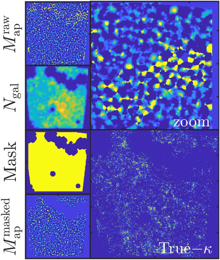
1624        J. Harnois-Déraps et al.
experiments, notably the Rubin observatory,4 and the Euclid5 and             must be carefully calibrated on numerical simulations specifically
Nancy Grace Roman6 space telescopes.                                         tailored to the data being analysed, which are generally expensive
   The central approach adopted by these surveys for constraining            to run. Faster approximate methods exist (e.g. Izard, Fosalba &
cosmology is based on two-point statistics – mostly either in the            Crocce 2018); however, they typically suffer from small scale
form of correlation functions (e.g. Kilbinger et al. 2013; Troxel            inaccuracies exactly in the regime where the lensing signal is the
et al. 2018; Hamana et al. 2020; Asgari et al. 2021) or its Fourier          strongest, introducing significant biases in the inferred cosmological
equivalent, the power spectrum, estimated using pseudo-C (Hikage            parameters. Previous peak count analyses of the third KiDS data
et al. 2019), band powers (Becker et al. 2016; van Uitert et al.             release (KiDS-450; Martinet et al. 2018, M18 hereafter) and of the
2018; Joachimi et al. 2021), and quadratic estimators (Köhlinger            DES Science Verification data (Kacprzak et al. 2016, K16 hereafter)
et al. 2017). By definition, these two-point functions can potentially       calibrated their signal on a suite of full N-body simulations spanning
capture all possible cosmological information contained in a linear,         the [m −σ 8 ] plane described in Dietrich & Hartlap (2010). The
Gaussian density field, and are thus highly efficient at analysing large     accuracy of this suite has however been later shown to be only
scale structure data. They have been thoroughly studied in terms of          ∼10 per cent (Giblin et al. 2018). Significant improvements on the

                                                                                                                                                        Downloaded from https://academic.oup.com/mnras/article/506/2/1623/6297283 by guest on 15 September 2021
signal modelling (Kilbinger et al. 2017), measurement (Schneider             simulation side are therefore critical for the new generation of data
et al. 2002; Jarvis, Bernstein & Jain 2004; Alonso et al. 2019) and          analyses based on non-Gaussian statistics.
systematics (Mandelbaum 2018).                                                   This paper aims to address this issue: we present a cosmolog-
   With the improved accuracy and precision provided by current and          ical re-analysis of the DES-Y1 cosmic shear data (Abbott et al.
upcoming surveys, it becomes increasingly appealing to probe small           2018b), exploiting a novel simulation-based cosmology inference
angular scales, where the signal is the strongest. In doing so, the          pipeline calibrated on state-of-the-art suites of N-body runs that are
measurements are intrinsically affected by the non-Gaussian nature           specifically designed to analyse current weak lensing data beyond
of the matter density field, and it is natural to seek analysis techniques   two-point statistics. In this work, the incarnation of our pipeline is
that can extract the additional cosmological information that two-           tailored for the peak count analysis of the DES-Y1 survey; however,
point functions fail to capture. A variety of alternative methods            it is straightforward to extend it to alternative non-Gaussian probes.
have been applied to lensing data with this in mind, including               Our pipeline first calibrates the cosmological dependence of arbi-
three-point functions (Fu et al. 2014), Minkowski functionals and            trary non-Gaussian measurements with the cosmo-SLICS (Harnois-
lensing moments (Petri et al. 2015), peak count statistics (Liu et al.       Déraps, Giblin & Joachimi 2019), a segment of the Scinet LIght-Cone
2015a,b; Kacprzak et al. 2016; Martinet et al. 2018; Shan et al. 2018),      Simulations suite that samples m , σ 8 , w0 , and h (the Hubble reduced
density split statistics (Gruen et al. 2018), clipping of the shear field    parameter). We next estimate the covariance from a suite of fully
(Giblin et al. 2018), convolutional neural networks (Fluri et al. 2019),     independent N-body runs extracted from the main SLICS sample7
and neural data compression of lensing map summary statistics                (Harnois-Déraps et al. 2018). We further use the cosmo-SLICS to
(Jeffrey, Alsing & Lanusse 2021). Other promising techniques are             generate systematics-infused control samples that we use to model
also being developed, notably the scattering transform (Cheng et al.         the impact of photometric redshift and shear calibration uncertainty.
2020), persistent homology (Heydenreich, Brück & Harnois-Déraps            We study the impact of galaxy intrinsic alignment with dedicated
2021), lensing skew-spectrum (Munshi et al. 2020), lensing minimas           mock data in which the ellipticities of central galaxies are aligned
(Coulton et al. 2020), and moments of the lensing mass maps (van             (or not) with the shape of their host dark matter haloes, following the
Waerbeke et al. 2013; Gatti et al. 2020).                                    in-painting prescription of Heymans et al. (2006; see also Joachimi
   While existing non-Gaussian data analyses revealed a constraining         et al. 2013b for a more recent application). We finally use a suite
power comparable to that of the two-point functions, it is expected          of high-resolution simulations (SLICS-HR, presented in Harnois-
that the gain will drastically increase with the statistical precision       Déraps & van Waerbeke 2015) to investigate the impact of mass-
ofthe data. For example, constraints on the sum of neutrino mass            resolution on the non-Gaussian statistics, and full hydrodynamical
( mν ), on the matter density (m ), and on the amplitude of the             simulation light-cones from the Magneticum Pathfinder8 to assess
primordial power spectrum (As ), in a tomographic peak count anal-           the effect of baryon feedback. All of the above are fully integrated
ysis of LSST, are forecasted to improve by 40 per cent, 39 per cent,         with the COSMOSIS cosmological inference pipeline (Zuntz et al.
and 36 per cent respectively, compared to a power-spectrum analysis          2015) and therefore interfaces naturally with the two-point statistics
of the same data (Li et al. 2019). Upcoming measurements of the              likelihood, enabling joint analyses with the fiducial DES-Y1 cosmic
dark energy equation of state (w 0 ) will also benefit from these            shear correlation function measurements presented in Troxel et al.
methods, with a forecasted factor of three improvement expected              (2018, T18 hereafter), with the 3 × 2 points analysis presented in
on the precision when combining two-point functions with aperture            DES Collaboration (2018), or any other analysis implemented within
mass map statistics (Martinet et al. 2021a). Similar results are found       COSMOSIS.
in the context of a final Stage-III lensing experiment such as the               The current document is structured as follow: In Section 2.1 we
(upcoming) DES-Y6 data release, where the combination of non-                present the data and the simulation suites on which our pipeline
Gaussian statistics with the power spectrum                                  is built; Section 3 describes the theoretical background, the weak
                                           √ method reduces the error
on the parameter combination S8 ≡ σ8 m /0.3 by about 25 per cent            lensing observables, and the analysis methods. A detailed treatment
compared to a two-point function (Zürcher et al. 2021), where σ 8 is        of our systematic uncertainties is presented in Section 4, the results
the normalization amplitude of the linear matter power spectrum.             of our DES-Y1 data analysis are discussed in Section 5, and we
   In the absence of accurate theoretical predictions for the signal, the    conclude afterwards. The appendices contain additional validation
covariance, and the impact of systematics, non-Gaussian statistics           tests of our simulations and further details on our cosmological
                                                                             inference results.

4 LSST:www.lsst.org
5 Euclid:
       sci.esa.int/web/euclid                                                7 slics.roe.ac.uk
6 WFIRST: roman.gsfc.nasa.gov                                                8 www.magneticum.org

MNRAS 506, 1623–1650 (2021)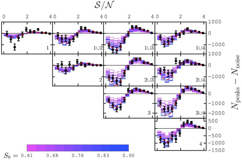
DES-Y1 cosmology beyond two-point statistics                              1625
                                                                                  (see Zuntz et al. 2018 for details). While they provide consistent
                                                                                  results, the former method has a larger acceptance rate of objects
                                                                                  with good shape measurements, and thereby results in measurements
                                                                                  with higher signal-to-noise. Following Troxel et al. (2018), we also
                                                                                  adopt the METACALIBRATION shear estimates in our analysis. This
                                                                                  method provides a shear response measurement per galaxy, Rγ ,
                                                                                  a 2 × 2 matrix that must be included to calibrate any measured
                                                                                  statistics (we refer to Zuntz et al. 2018 for more details on this
                                                                                  calibration technique in the context of shear two-point correlation
                                                                                  functions). Additionally, the galaxy selection itself can introduce a
                                                                                  selection bias, which can be captured by a second 2 × 2 matrix,
                                                                                  labelled RS in T18, which we choose not to include due to the
                                                                                  small relative contribution. We compute from these matrices the

                                                                                                                                                                   Downloaded from https://academic.oup.com/mnras/article/506/2/1623/6297283 by guest on 15 September 2021
                                                                                  shear response correction, defined as S = Tr(Rγ )/2. As explained
                                                                                  in T18, the method imposes a prior on an overall multiplicative shear
Figure 1. Tiling strategy adopted to pave the full DES-Y1 data (black) with
                                                                                  correction of m ± σ m = 0.012 ± 0.023, which calibrates the galaxy
flat-sky 10 × 10 deg2 simulations (red squares). The squares overlap owing
                                                                                  ellipticities as  →  (1 + m), with  ≡ 1 + i2 .
to the sky curvature, hence we separate the data at the mean declination in the
overlapping regions. In our pipeline, measurements are carried out in each            The galaxy sample is further divided into four tomographic redshift
tile separately, then combined at the level of summary statistics.                bins based on the photometric redshift posterior estimated from griz
                                                                                  flux measurements (Hoyle et al. 2018). The redshift distribution in
2 DATA A N D S I M U L AT I O N S                                                 these bins, ni (z), must then be estimated, and a number of methods
                                                                                  are proposed to achieve this. The fiducial cosmic shear results
We present in this section the data and simulations included in our               presented in T18 are based on the Bayesian photometric redshift
analysis. We exploit multiple state-of-the-art simulation suites in               (BPZ) methodology described in Benı́tez (2000), which are consistent
order to conduct our cosmological analysis, including a Cosmology                 with a n(z) estimated by resampling the COSMOS2015 field (Laigle
training set to model the response of our measurement to variations               et al. 2016) with objects of matched flux and size (Hoyle et al. 2018).
in cosmology, as well as a Covariance training set and multiple Sys-              However, the accuracy of these two methods has been questioned
tematics training sets. These DES-Y1-specific simulation products                 in Joudaki et al. (2020, J20 hereafter), where it is argued that even
are created from four suites of simulations, which we describe after              though both the BPZ and COSMOS resampling estimates account for
introducing the data.                                                             statistical uncertainty, residual systematics effects could significantly
   The total computing cost of the SLICS, cosmo-SLICS, and SLICS-                 affect the inferred n(z) distributions. In particular, the COSMOS
HR are 12.3, 1.1 and 1.3 million CPU hours, respectively. They                    sample could be populated with outliers and/or an overall bias that
were produced on a system of IBM iDataPlex DX360M2 machines                       would affect the calibration (e.g. fig. 11 of Alarcon et al. 2021),
equipped with one or two Intel Xeon E5540 quad cores, running                     and J20 proposes instead to calibrate with redshifts from matched
at 2.53 GHz with 2 GB of RAM per core. Every simulation was                       spectroscopic catalogues.10 The direct reweighted estimation method
split into 64 MPI processes, each further parallelised with either four           (Lima et al. 2008, DIR hereafter) was selected for the fiducial cosmic
or eight OPENMP threads. Modern compilers and CPUs would likely                   shear analysis of the third KiDS data release (Hildebrandt et al. 2017,
bring the total computing cost down if similar simulations had to be              2020), and for the DES-Y1 data re-analyses of J20 and Asgari et al.
run again in the future.                                                          (2020), where it is found that this calibration brings both DES-Y1 and
                                                                                  KV450 results in excellent agreement, affecting the constraints on S8
                                                                                  by only 0.8σ . It should be noted also that DIR has inherent systematic
2.1 DES-Y1 data
                                                                                  uncertainties that are hard to quantify. In particular, incomplete
In this paper we present cosmological constraints obtained from a re-             spectroscopy and colour pre-selection (Gruen & Brimioulle 2017)
analysis of the public lensing catalogues of the Year-1 data release9 of          can potentially bias the DIR n(z). Despite these issues that can in
the Dark Energy Survey (Abbott et al. 2018b). These catalogues were               principle be addressed by a pre-selection of sources via the self
obtained from the analysis of millions of galaxy images taken by the              organizing map technique (Wright et al. 2020), we choose to adopt
570 megapixel DECam (Flaugher et al. 2015) on the Blanco telescope                this DIR methodology for simplicity and to be able to easily relate
at the Cerro Tololo Inter-American Observatory, observed in the                   our findings to previous work. We use the same tomographic redshift
grizY bands. The specific selection criteria of the DES-Y1 cosmic                 distribution ni (z) and uncertainty about the mean redshift zDIR i
                                                                                                                                                        as
shear data used in this paper exactly match those of the cosmic shear             in J20 here. In this method, the uncertainties on the mean redshifts,
analysis presented in Troxel et al. (2018): they consist of 26 million            σzi , are estimated from a bootstrap resampling of the spectroscopic
galaxies that pass the FLAGS SELECT, METACAL, and the REDMAGIC                    samples. The density, the mean redshifts, and the shape noise of the
filters (Zuntz et al. 2018), thereafter covering a total unmasked area of         galaxies in individual tomographic bins are presented in Table 1.
1321 deg2 , for an object density of 5.07 gal arcmin−2 . The footprint
of the DES-Y1 data is presented in Fig. 1, which shows in black the
galaxy positions from the selected sample.                                        10 Both the DIR and the COSMOS resampling methods have been shown to be
    The galaxy shears in the DES-Y1 data are estimated by two
                                                                                  consistent with other n(z) estimation techniques such as the cross-correlation
independent methods, METACALIBRATION (Sheldon & Huff 2017)                        between photometric and overlapping spectroscopic surveys (Morrison et al.
and IM3SHAPE (Zuntz et al. 2013) that were both fully implemented                 2017; Johnson et al. 2017; Hoyle et al. 2018; Gatti et al. 2020; Hildebrandt
                                                                                  et al. 2020). J20 also show that the DIR method is robust against the specific
                                                                                  choice of spectroscopic calibration sample, provided that the combination is
9 des.ncsa.illinois.edu/releases/dr1                                              sufficiently wide and deep.

                                                                                                                         MNRAS 506, 1623–1650 (2021)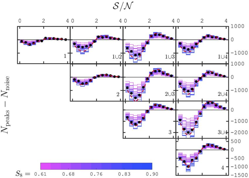
1626           J. Harnois-Déraps et al.
Table 1. Survey properties. The effective number densities neff (in                Two of these models (cosmology-fid and -00; see HD19) are
gal arcmin−2 ) and shape noise σ  listed here assume the definition of Chang    used to infuse photometric redshift and shear calibration uncertainty,
et al. (2013). The column ‘ZB range’ refers to the photometric selection that    which we describe in Section 4.1 and 4.2, respectively.
defines the four DES-Y1 tomographic bins, while the mean redshift in each
bin is listed under zDIR .
                                                                                 2.3 Covariance training set
tomo         ZB range     No. of objects     neff     σ          zDIR
                                                                                 Our covariance matrix is estimated from the SLICS (Harnois-Déraps
bin1         0.20–0.43       6993 471        1.45     0.26    0.403 ± 0.008      et al. 2018, HD18 hereafter), a public simulation suite in which the
bin2         0.43–0.63       7141 911        1.43     0.29    0.560 ± 0.014      cosmology is fixed for every N-body run, but the random phases in the
bin3         0.63–0.90       7514 933        1.47     0.26    0.773 ± 0.011      initial conditions are varied, offering a unique opportunity to estimate
bin4         0.90–1.30       3839 717        0.70     0.27    0.984 ± 0.009      the uncertainty associated with sampling variance. The volume and
                                                                                 number of particles are the same as for the cosmo-SLICS, achieving a
                                                                                 particle mass of 2.88 h−1 M (see the properties summary in Table 2).

                                                                                                                                                            Downloaded from https://academic.oup.com/mnras/article/506/2/1623/6297283 by guest on 15 September 2021
Table 2. Summary of key properties from the four simulations suites used in      The light-cones are constructed in the same way as the cosmo-
our pipeline. Lbox is the box side (in h−1 Mpc), np is the number of particles   SLICS, except that in this case the mass sheets are sampled only once
evolved, Nsim is the number of N-body runs, NLC is the number of light-cones     per N-body run, generating 124 truly independent realizations. The
in the full training set, and Ncosmo is the number of cosmology samples.         accuracy of the SLICS has been quantified in Harnois-Déraps & van
The bottom section summarizes the range in cosmological parameters that is       Waerbeke (2015) by comparing their matter power spectrum to that of
covered by the cosmo-SLICS.                                                      the Cosmic Emulator (Heitmann et al. 2014), which match to within
                                                                                 2 per cent up to k = 2.0 hMpc−1 ; smaller scales progressively depart
Sim. suite                  Lbox            np        Nsims    NLC    Ncosmo
                                                                                 from the emulator. The cosmo-SLICS have a similar resolution.
cosmo-SLICS                  505           15363        52     520          26
SLICS                        505           15363       124     124          1
                                                                                 2.4 Systematics training set: mass resolution
SLICS-HR                     505           15363        5       50          1
Magneticum 2                 352        2 × 15833       1       10          1    Numerical simulations are inevitably limited by their intrinsic mass
Magneticum 2b                640        2 × 28803       1       10          1    and force resolution, and it is critical to understand how these affect
Parameter                    m              S8               h     w0           any measurements carried out on the simulated data. We employ
Sampling                 [0.1, 0.55]     [0.6, 0.9]   [0.6, 0.82] [−2.0, −0.5]
                                                                                 for this purpose a series of ‘high-resolution’ runs, first introduced
                                                                                 in Harnois-Déraps & van Waerbeke (2015) and labelled ‘SLICS-
                                                                                 HR’ therein. These consist of five independent N-body simulations
                                                                                 similar to the main SLICS suite, but in which the force accuracy of
2.2 Cosmology training set
                                                                                 CUBEP3 M has been increased significantly such as to resolve smaller
The training set is constructed from the cosmo-SLICS (Harnois-                   structures, even though the particle number is fixed. These have been
Déraps, Giblin & Joachimi 2019, HD19 hereafter), a suite of w cold              shown to reproduce the Cosmic Emulator power spectrum to within
dark matter (CDM) N-body simulations specifically designed for                   2 per cent up to k = 10.0 h−1 Mpc, indicating that even those small
weak lensing data analysis targeting dark matter and dark energy.                scales are correctly captured by the simulations. The SLICS-HR are
These simulations cover a wide range of values in (m , σ 8 , h, w0 ).           post-processed with a strategy similar to that adopted for the cosmo-
They sample the parameter volume at 25 + 1 coordinates organized                 SLICS, re-sampling the projected mass sheets in order to generate
in a Latin hypercube (25 wCDM plus one CDM point), and further                   10 pseudo-independent light-cones per run.
include a sample variance suppression technique, achieving a sub-
per cent to a few per cent accuracy depending on the scales involved.
                                                                                 2.5 Systematics training set: baryon feedback
This is comparable to the accuracy of many widely-used two-point
statistics models based on non-linear power spectra from HALOFIT                 Another important systematic we investigate in this analysis is
(Takahashi et al. 2012) or from HMCODE (Mead et al. 2015, 2021).                 the impact of strong baryonic physics that modifies the clustering
The full training range is detailed in Table 2, which also influences            property of matter. As noted in multiple independent studies, active
our choice of priors when sampling the likelihood (see Section 3.6).             galactic nucleus (AGN) feedback has a particularly important effect
   Each run evolved 15363 particles inside a 505 h−1 Mpc co-moving               on the matter power spectrum but is challenging to calibrate.
volume with the public CUBEP3 M N-body code (Harnois-Déraps et al.              Simulations often struggle to reproduce the correct baryon fraction in
2013), generating on-the-fly multiple two-dimensional projections                haloes of different masses, and these differences in turn cause major
of the density field. These flat-sky mass planes were subsequently               discrepancies in the clustering properties (see Chisari et al. 2018
arranged into past light-cones of 10 degrees on the side, from which             for example). In this paper, we examine one of these models and
lensing maps were extracted at a number of redshift planes (see                  inspect which parts of our peak count measurements are affected by
Section 2.6.1). This process was repeated multiple times after the               baryons.
mass planes were randomly selected from a pool of six different                     We used for this exercise a series of light-cones ray-traced from
projected sub-volumes, then their origins were randomly shifted. In              a subset of the Magneticum Pathfinder hydrodynamical simulations
total, 50 pseudo-independent light-cones per cosmology are available             that are designed to study the formation of cosmological structures
for the generation of galaxy lensing catalogues (see HD19 for a                  in presence of baryonic physics and that were recently described
complete description). In the end we include 10 light-cones per                  in Castro et al. (2021). These are based on the smoothed particle
cosmology out of 50, after verifying that our results do not change              hydrodynamics code P-GADGET3 (Springel 2005), in which a number
when training on only five of them. Indeed, 1000 deg2 is enough                  of baryonic processes are implemented, including radiative cooling,
to reach convergence on our statistics, largely due to the sample                star formation, supernovae, AGN, and their associated feedback on
suppression technique implemented in HD19.                                       the matter density field. The Magneticum reproduce a number of

MNRAS 506, 1623–1650 (2021)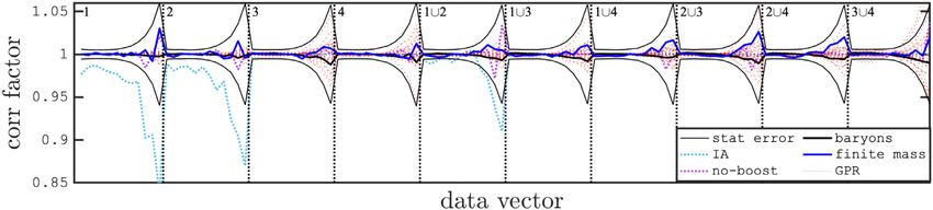
DES-Y1 cosmology beyond two-point statistics                                 1627
key observations such as statistical properties of the large-scale,          are divided into smaller ‘tiles’11 that all fit inside 100 deg2 square
intergalactic, and intercluster medium, but also central dark matter         areas. Each of these tiles are then overlaid with simulated light-
fractions and stellar mass size relations (see Hirschmann et al. 2014;       cones from which lensing quantities are extracted. In total, 19
Teklu et al. 2015; Castro et al. 2018, 2021 for more details). What is       tiles are required to assemble the full footprint with our mosaic,
especially important in our case is that the total baryonic feedback on      which is shown in Fig. 1. Every simulated light-cone from the
the matter field is comparable to that of the BAHAMAS cosmological           Cosmology, Covariance, or Systematics training sets is therefore
hydrodynamical simulations (McCarthy et al. 2017), in particular in          replicated 19 times and associated with a full realization of the
terms of the strength of the effect on the matter power spectrum. This       survey.
derives from the similar baryon fractions produced by Magneticum                We emphasize that the simulated light-cones are discontinuous
and BAHAMAS that are in reasonable agreement with observations.              across tile boundaries, whereas data are not. To avoid significant
This validates the Magneticum as a good representation for the impact        calibration biases caused by this difference, no measurement what-
of baryon feedback, given the current uncertainty on the exact impact        soever must extend over tile boundaries. Both data and mock data
(see Section 4.3 for further discussion).                                    are separated in tiles at the catalogue level; these are then analysed

                                                                                                                                                                 Downloaded from https://academic.oup.com/mnras/article/506/2/1623/6297283 by guest on 15 September 2021
   Among the various runs, we use a combination of the high-                 individually, and the data vectors are combined at the end.12
resolution Run-2 (Hirschmann et al. 2014) and Run-2b (Ragagnin                  Another subtle difference that needs to be taken into account is
et al. 2017), which both co-evolve dark matter particles of mass             that the position coordinates (RA, Dec) and the galaxy ellipticities
6.9 × 10⁸ h−1 M and gas particles with mass 1.4 × 10⁸ h−1 M in               () from the data are provided on the (southern) curved sky, whereas
comoving volumes of side 352 and 640 h−1 Mpc, respectively; the              all of our simulations assume a (X, Y) Cartesian coordinate system.
smaller (larger) box is used at lower (higher) redshift, and the             Since the physics are independent of our choice of coordinate system,
transition occurs at z = 0.31. The input cosmology is consistent             and since we analyse every tile individually, we apply a coordinate
with the SLICS but slightly different, with m = 0.272, h = 0.704,           transformation to centre every tile on to the equator, where both
b = 0.0451, ns = 0.963, and σ 8 = 0.809. Both Run-2 and Run-2b              coordinate frames converge.13 The weak lensing statistics of a given
also exist in pure gravity mode (i.e. dark matter only) with otherwise       tile are unaffected by this rotation, a fundamental fact that we verify
identical initial conditions, allowing us to isolate the impact of the       with two-point correlation functions in Section 3.1.
baryonic sector on our observables.                                             As easily noticed from looking at Fig. 1, some of the galaxies fall
                                                                             outside the tiles, which slightly affects the total number of galaxies
                                                                             in the sample. It is not ideal, but adding multiple simulated tiles for
2.6 Simulation post-processing                                               such a small fraction (1.9 per cent) of the data is arguably not worth
                                                                             the effort. The number of objects listed in Table 1 reflects this final
2.6.1 Light-cones
                                                                             selection and amounts to a total of 25.5 million of galaxies.
The simulation suites used in this paper all work under the flat sky
approximation that assumes that the maps are far enough from the ob-
server so that Cartesian axes can be used instead of angles and radial       2.6.3 Mock galaxy shapes and redshifts
distances. At pre-selected redshifts z, the N-body/hydrodynamical            As mentioned above, the position and the intrinsic ellipticities of
codes assign the particles on to a three-dimensional grid, select a sub-     individual galaxies in the simulated catalogues are taken from the
volume to be projected with pre-determined co-moving thickness,              observations. Redshifts are assigned to every object in a given
and collapse the mass density along one of the axis. This procedure          tomographic bin ‘i’ by sampling randomly the ni (z) described in
is repeated with different projection directions and sub-volumes,            Section 2.1. Therefore, variations in survey depth are not included
creating a collection of mass sheets at every redshift. These are next       in our training sets. This induces a systematic difference with the
post-processed to generate a series of past light-cone mass maps,            data, but we expect that this has a minor effect on our cosmological
δ2D (θ , z), each of 100 deg2 , that are then used to generate convergence   measurement. Indeed, it was shown in Heydenreich et al. (2020) that
κ(θ, zs ) and shear γ (θ , zs ) maps at multiple source redshift planes,     the impact of survey depth variability is subdominant for Stage-III
zs , (see HD18 and HD19 for full details), where γ = γ1 + iγ2 , the          surveys. At this stage, every galaxy has position and a redshift that
two components of the spin-2 shear field. From these, mock lensing           are used to extract the lensing quantities (κ, γ ) from the simulation
quantities (κ, γ ) can be computed for any galaxy position provided          light-cones.
its (RA, Dec) coordinates and a redshift.                                       We finally include the intrinsic galaxy shapes and METACAL shear
                                                                             response correction in the simulations by randomly rotating the

2.6.2 Assembling the simulated surveys                                       11 These  tiles are sometimes called ‘patches’ in the literature, e.g. in K16.
As for many non-Gaussian statistics, peak counts are highly sensitive        12 Note  that the tiles are identical for all simulations (SLICS, cosmo-SLICS,
to the noise properties of the data. As such the simulations need to         SLICS-HR, and Magneticum) since their light-cones all have the same
reproduce exactly the position and shape noise of the real data,             opening angle.
                                                                             13 In this process, we rotate both the celestial coordinate and the ellipticities
otherwise the calibration will be wrong. The solution, adopted in
                                                                             of every galaxy in the tile to account for the modified distance to the South
Liu et al. (2015a), K16, and M18 is to overlay data and simulated
                                                                             pole in the new coordinate frame. The exact transformation uses the method
light-cones, and to construct mock surveys from the position and
                                                                             presented in the appendix B of Xia et al. (2020), which rotates pairs of galaxies
intrinsic shape of the former, and the convergence and shear of the          from any orientation on the sky on to the equator, placing one member at the
latter.                                                                      origin. In our case we instead map to the equator the straight line that bisects
   Since the size of the full DES-Y1 footprint largely exceeds that          every tile. Every tile has its unique rotation vector, which we also use to
of our individual light-cones, we connect the data and simulations           displace the galaxies and to recompute their ellipticities ( 1/2 ) in this new
with a ‘mosaic’ approach, where the DES-Y1 galaxy catalogues                 coordinate frame.

                                                                                                                      MNRAS 506, 1623–1650 (2021)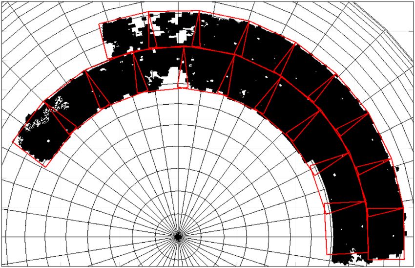
1628          J. Harnois-Déraps et al.
observed galaxy shapes such as to undo the cosmological correlations     that computes shape correlations between pairs of galaxies ‘a, b’
from the data, and we then combine the new ellipticity  int with the    separated by an angle ϑ as
simulated lensing signal as
                                                                                                            j                        j
                                                                                     ab Wa Wb a,t (θ a ) b,t (θ b ) ± a,× (θ a ) b,× (θ b ) ϑab
                                                                                                 i                       i
      int + g                                                            ij

=                .                                               (1)    ξ± (ϑ) =                                                                    .
     1 +  ∗int g                                                                                          ab Wa Wb Sa Sb

Here g is the reduced shear, defined as g = γ S/(1 + κ), and the bold-                                                                               (5)
font symbols g, γ , , and  int are again spin-2 complex quantities.    In the above expression, the sums are over all galaxies ‘a’ in
  We investigate in Section 4.4 the impact of the intrinsic alignment    tomographic bin i and galaxies ‘b’ in tomographic bin j; a,t      i
                                                                                                                                              , and
of galaxies where  int is no longer chosen at random and instead         i
                                                                         a,×  are the tangential and cross components of the ellipticity of
correlates with the shape of dark matter haloes.                         galaxy a in the direction of galaxy b; Wa/b are weights attributed to
                                                                         individual galaxies, which are set to unity in the METACALIBRATION
                                                                         shear inference method; Sa/b are the ‘shear response correction’

                                                                                                                                                           Downloaded from https://academic.oup.com/mnras/article/506/2/1623/6297283 by guest on 15 September 2021
3 T H E O RY A N D M E T H O D S
                                                                         per object mentioned in Section 2.1 and provided in the DES-Y1
Since we validate our simulation suites with cosmic shear correlation    catalogue; ϑab is the binning operator, which is equal to unity if
functions and lensing power spectra, we begin this section with a        the angular separation between the two galaxies falls within the ϑ-
review of the theoretical modelling and the measurement strategies       bin, and zero otherwise. Our raw measurements are organized in 32
related to these quantities. We next move to the primary focus of        logarithmically spaced ϑ-bins, in the range [0.5–475.5] arcmin, but
this paper and describe our peak count statistics pipeline, detailing    not all angular scales are used in this work.15
our treatment of the data, our approach to modelling the signal,                                                               ij
                                                                            We present in Fig. 2 our measurements of ξ± on the DES-Y1
and estimating the covariance matrix, and we finally describe our        data, showing with the black solid points the measurement on the
cosmological inference methods.                                          full footprint, and with the open blue triangles the measurements on
                                                                         the 19 data tiles described in Section 2.6.2 that are combined with a
3.1 ξ ± statistics                                                       weighted mean using the TREECORR Npairs (ϑ) per tile as our weights.
                                                                         We see that the two results are similar, with differences that are
Two-point correlation functions (2PCFs) are well studied and have a      everywhere at least twice as small as the statistical error measured
key advantage over other measurement techniques: as for all lensing      from the covariance mocks (see below) and evenly scattered about
two-point statistics, their modelling can be accurately related to       the black points, validating our tiling method. We further verified
the matter power spectrum, P(k, z), whose accuracy is reaching           that the difference on the inferred cosmology is negligible (see
the per cent level far in the non-linear regime when calibrated with     Section 5).
N-body simulations at small scales, and in absence of baryonic              We also show, with the red squares in Fig. 2, the mean, and
physics (Heitmann et al. 2014; Euclid Collaboration: Knabenhans          expected 1σ error on the DES-Y1 data as estimated from the Covari-
& the Euclid Collaboration 2019). From this P(k, z), the lensing         ance training set. The agreement between theory and simulations is
power spectrum between tomographic bins ‘i’ and ‘j’ is computed          excellent at all scales, and the slight differences are well under the
in the Limber approximation as                                           statistical precision of the data. We can observe a slight loss of power
        χH i                                                          at large angular scales in the ξ + statistics, a finite box effect that we
  ij         q (χ ) q j (χ )      + 1/2
C =                         P           , z(χ )   dχ ,          (2)     forward model (see Appendix A1). For every simulated light-cone
         0        χ2                χ
                                                                         we generate a total of 10 realizations of the shape noise by rotating,
where χ H is the co-moving distance to the horizon, and the lensing      as many times, every galaxy in the catalogue, and recomputing new
kernels qi are computed from the redshift distributions n(z) as          observed ellipticities (with equation 1) and the correlation functions
                 2         χH                                         (equation 5). The red squares in Fig. 2, as well as their associated
          3      H0     χ                 dz χ − χ
q i (χ ) = m                     ni (χ )            dχ ,       (3)      error bars, correspond to one of these realizations; we observe no
          2       c    a(χ ) χ            dχ    χ                        significant change in the other nine realizations, and recover the
where c and H0 are the speed of light and the Hubble parameter,          error bars reported by T18 to within 5–15 per cent over most angular
                                                         ij              scales, further demonstrating the robustness of our training set. We
respectively. The cosmic shear correlation functions ξ± are
                     ij                                                  do not expect a perfect match due to the slightly different binning
computed from the C as
               ∞                                                        scheme.
 ij        1       ij                                                       Our cosmological analyses exclude the same angular scales as in
ξ± (ϑ) =          C J0/4 (ϑ)  d,                        (4)
          2π 0                                                           T18, removing the elements of the data vector where T18 conclude
with J0/4 (x) being Bessel functions of the first kind. Following T18,   that the uncertainty on the baryonic feedback and in the non-linear
equation (4) is solved with the cosmological parameter estimation        matter power spectrum is non-negligible. These scales are indicated
code COSMOSIS14 (Zuntz et al. 2015), in which the matter power           by the vertical lines in Fig. 2.
spectrum is calculated by the HALOFIT model of Takahashi et al.             The variation of ξ ± with cosmology are well captured by COS-
                 ij
(2012). The ξ± predictions for the DES-Y1 measurements are               MOSIS, and so are the responses to photometric redshift and shear
shown by the black lines in Fig. 2 for all pairs of tomographic bins,    calibration uncertainties (see Section 4). We therefore do not measure
at the SLICS input cosmology.                                            this statistic in the Cosmology nor the Systematics training sets, and
                           ij                                           use instead the public modules provided in the latest COSMOSIS
   The measurements of ξ± from simulations and data are carried
                                                                         release to calculate these.
out with TREECORR (Jarvis et al. 2004), a fast parallel tree-code

14 bitbucket.org/joezuntz/cosmosis/wiki/Home                             15 Note   that T18 used 20 logarithmic bins in the range 2.5–250 arcmin.

MNRAS 506, 1623–1650 (2021)
DES-Y1 cosmology beyond two-point statistics 1629
101 102 101 102 101 102 101 102
2
1
0
4 4
2 2
0 0
4 4
2 2
0 0
Downloaded from https://academic.oup.com/mnras/article/506/2/1623/6297283 by guest on 15 September 2021
4
4
2
2
0
0
2
1 DES-Y1 footprint
DES-Y1 tiles
0
SLICS
-1 Theory
101 102 101 102 101 102 101 102
Figure 2. Two-point correlation functions measured in the DES-Y1 data (filled circles and opened triangles present measurements on the full survey footprint
and from a weighted mean over the tiles presented in Fig. 1, respectively) and in the SLICS simulations (red squares, with error bars showing the statistical error
on the DES-Y1 data), compared to the analytical model computed at the input SLICS cosmology (solid lines). The left- and right-hand side ladder plots present
the ξ − and ξ + statistics, respectively, and the sub-panels in each correspond to different combinations of tomographic bins. The vertical dotted lines indicate
the angular scales excluded in the cosmological analysis, which match those of T18.
3.2 Shear peak count statistics where ngal (θ) is the galaxies density in the filter centred at θ ,
and θ a is the position of galaxy a. The tangential ellipticity
As mentioned in the introduction, the peak count statistic is a
with respect to the aperture centre is computed as a,t (θ , θ a ) =
powerful alternative method to extract cosmological information
−[1 (θ a ) cos(2φ(θ, θ a )) + 2 (θ a ) sin(2φ(θ, θ a ))], where φ(θ , θ a ) is
from weak lensing data. It consists of measuring the ‘peak function’,
the angle between both coordinates. Our filter Q(θ, θ ap , xc ), abridged
i.e. the number of lensing peaks as a function of their signal-to-noise,
to Q(θ) to shorten the notation, is identical to that in Schirmer et al.
which is very sensitive to cosmology and robust to systematics [see
(2007), which is optimal for detecting haloes following an NFW
Zürcher et al. (2021) Martinet et al. (2021a) for recent comparisons
profile (but faster than solving the actual numerical NFW equation),
with other lensing probes].
Our measurement technique closely follows that described in K16 tanh(x/xc ) −1
and M18, which we review here. Peaks are identified from local Q(x) = 1 + exp(6 − 150x) + exp(−47 + 50x) . (7)
x/xc
maxima in the signal-to-noise maps of the mass within apertures
(Schneider 1996), Map (θ ), searching for pixels with values higher In the above expression, x = θ/θ ap , where θ is the distance to the filter
than their eight neighbours. This is one of many ways to estimate centre, and we adopt xc = 0.15 as in previous works, a choice that
the projected mass map from galaxy lensing catalogues, and was maximizes the sensitivity of the signal to the massive haloes, which
chosen primarily for its local response to data masking. This is to be carry the majority of the cosmological information. The filter size of
contrasted with e.g. the Fourier methods of Kaiser & Squires (1993) θ ap = 12.5 arcmin is adopted as in M18; however, we also consider
in which masking introduces a complicated mode-mixing matrix 9.0 and 15.0 arcmin, and report results for these where appropriate.
that can affect all scales. Other techniques such as Bayesian mass Hereafter, equation (6) defines the signal of our aperture mass map,
reconstruction (Price et al. 2021) or wavelets transforms (Leistedt which we compute at every pixel location.
et al. 2017) are also promising and merit to be explored in the future The variance about this map is calculated at every pixel location
(see as well Gatti et al. 2020, and references therein). from
From a lensing catalogue containing the position, ellipticity a and 1
shear response correction Sa per galaxy, we construct an aperture
2
σap (θ) = 2 | a |2 Q2 (|θ − θ a |), (8)
mass map on a grid by summing16 over the tangential component of 2n2gal (θ) a Sa a
the ellipticities from galaxies surrounding every pixel at coordinate
θ, weighted by an aperture filter Q. More precisely, we compute where again the sum runs over all galaxies in the filter. Note that
the magnitude of the measured galaxy ellipticities that enters this
1
Map (θ ) = a,t (θ , θ a )Q(|θ − θ a |, θap , xc ), (6) equation must also be calibrated by the shear response correction
ngal (θ ) a Sa a (see the appendix A of Asgari et al. 2020), hence the term [ a Sa ]2
in the denominator. The signal-to-noise map from which peaks are
identified, M(θ) ≡ S/N, is computed by taking the ratio between
16 In practice, we use a link-list to loop only over nearby galaxies. equation (6) and the square root of equation (8) at every pixel
MNRAS 506, 1623–1650 (2021)1630 J. Harnois-Déraps et al.
in the aperture filter, ngal (θ), and require that it exceeds a fixed
threshold in order to down-weight or reject heavily masked apertures.
In this method, pixels with little or no galaxies are treated as masked.
We opted for the second method, setting the threshold to 1/π 2
gal arcmin−2 after a few different trials, which directly identifies
regions with very low galaxy counts. We further augment the masking
selection with an apodization step that flags as ‘also masked’ any
pixel within a distance θ ap of a masked region found in the first step.
Fig. 3 illustrates this procedure for one of the tiled catalogues,
for an idealized noise-free case. For our fiducial choice of filter
θ ap = 12.5 arcmin, we show in the upper two left-hand panel the
‘raw’ Map (θ) map (e.g. before masking, computed directly from
equation 6) as well as Ngal (θ). The masked regions are clearly visible
Downloaded from https://academic.oup.com/mnras/article/506/2/1623/6297283 by guest on 15 September 2021
in the latter but not so much in the former. A close inspection (top
right-hand panel), however, reveals overly smooth features in Map (θ ),
in regions where there are no galaxies (i.e. in the blue regions of the
Ngal (θ) map). The third left-hand panel shows the masked regions
constructed from our pipeline that is finally applied on the raw
aperture map, resulting in the masked map shown on the bottom
panel. All choices of θ ap result in aperture maps that closely recover
the true convergence (shown in the bottom right-hand panel).
It is clear from Fig. 3 that the unmasked area of our final maps
is affected by the aperture filter size. Indeed, larger filters can be
blind to small features in the mask, while the survey edges are more
severly excluded. This does not bias our cosmological inference since
we apply the same filter to the data and the simulations, but it does
Figure 3. Example of the Map mass-reconstruction pipeline over one of our slightly affect the signal-to-noise of our measurement that increases
10 × 10 deg2 tiles. The larger panel on the bottom right presents the true κ with the area of the survey. The net unmasked area in our final maps
values at the position of the galaxies in this field, extracted from the cosmo-
are (1426, 1408, 1366, 1327, 1284) deg2 for θ ap = (6.0, 9.0, 12.5,
SLICS model-00. The raw Map map is shown in the top left-hand panel in
the noise-free case. The number of galaxies in the filter (second panel) are
15.0, 18.0), respectively.
then used to construct a mask (third panel), which we apply on the raw Map
maps (bottom panel). The top right-hand panel shows a zoom-in of the top
left-hand panel, highlighting the effect of masking on the raw reconstructed 3.2.2 Peak function
Map map.
Peaks found in the (masked) M maps are counted and binned as a
location, e.g. function of their pixel value, thereby measuring the peak function
M(θ) ≡ Map (θ )/σap (θ ). (9) Npeaks (S/N). We use 12 bins covering the range 0 < S/N ≤ 4 in
our main data vector, which was found in K16 and M18 to avoid
Peaks catalogues are first constructed from the galaxy catalogues scales where multiple systematics uncertainties such as the effects of
separated in tomographic bins (which we label 1, 2, 3, and 4), and baryon feedback and intrinsic alignments of galaxies become large
then from every combination of pairs of tomographic catalogues (we extend this range to higher S/N values in some of our systematics
(which we label 1∪2, 1∪3, 1∪4 ... 3∪4). As detailed in Martinet investigations). 12 bins is also a good trade-off between our need
et al. (2021a), analysing these ‘cross-tomographic’ catalogues pro- to capture most cosmological information from Npeaks (S/N), while
vides additional information that is not contained within the ‘auto- keeping a small data vector for which the covariance matrix will be
tomographic’ case. They went further and also included triplets less noisy. A number of recent studies (M18; Davies, Cautun & Li
(1∪2∪3, 1∪2∪4, 1∪3∪4...) and quadruplets (1∪2∪3∪4), showing 2019; Coulton et al. 2020; Davies et al. 2020; Martinet et al. 2021a;
that these also contained additional information, but this gain is not Zürcher et al. 2021) have shown that cosmological information is
as significant in our case, where the noise levels are much higher. contained in peaks of negative S/N or in lensing voids; however, as
noted in appendix B of M18, the peaks with negative S/N strongly
correlate with those of positive S/N value, and only marginally
3.2.1 Masking
improve the constraints from peak statistics in the case of Stage-
Weak lensing data are taken inside a survey footprint, and parts of III surveys. We therefore focus only on the positive peaks in this
the images are removed in order to mask out satellite tracks, bright DES-Y1 analysis.
stars, saturated foreground galaxies, etc. The effect of data masking We show in Fig. 4 the peak function measured from the Cosmology
on the aperture mass map can be significant: the signal and the noise training set with θ ap = 12.5 arcmin, for all pair combinations of
are coherently diluted in apertures that strongly overlap with masked the four redshift bins and colour coded as a function of the input
regions, generating regions where M is overly smooth. Therefore the S8 . A pure noise case (Nnoise ), obtained from the average peak
survey mask must be included in the simulations and in the estimator function after setting γ = 0 on 10 full survey realizations, has been
such as to avoid biasing the statistics. subtracted to highlight the cosmological variations. Off-diagonal
If the masked pixels are known, this can be taken into account by panels present the cross-tomographic measurements. The colour
avoiding pixels for which e.g. more than half of the filter overlaps gradient is clearly visible in all tomographic bins; more precisely, all
with masked areas. Alternatively, one can examine the object density cosmologies present an excess of large S/N peaks and a depletion
MNRAS 506, 1623–1650 (2021)DES-Y1 cosmology beyond two-point statistics 1631
Downloaded from https://academic.oup.com/mnras/article/506/2/1623/6297283 by guest on 15 September 2021
Figure 4. Peak function Npeaks (S/N) in the DES-Y1 data (black squares) and simulations (coloured histograms), from which the expectation from pure shape
noise Nnoise (S/N) has been subtracted. The panels show different tomographic bin combinations, as labelled in their lower-right corners. The predictions are
colour coded by their S8 value, with the red dashed line showing the best-fitting value. The DES-Y1 error bars are estimated from the Covariance training set.
of low S/N peaks compared to pure noise. This is caused by the (iii) We deploy a fast emulator (see Section 3.5) that can model the
gravitational lensing signal that create peaks and troughs in the signal at arbitrary cosmologies within the parameter volume included
Map map and smooths out the smallest peaks. Importantly, these in the training. In contrast with a likelihood interpolator, emulating
differences are accentuated for high-S8 cosmologies. Also shown the data vector directly allows us to combine the summary statistics
with black squares are the measurements from the DES-Y1 data, with other measurement methods such as the two-point correlation
with error bars estimated from the Covariance training set. These functions, to better include systematic uncertainties, and to easily
demonstrate that most of the constraining power comes from the interface with most likelihood samplers;
auto-tomographic bins 3 and 4 and from the cross-tomographic bins. (iv) We generate a Covariance training set from a larger ensemble
Some additional information is contained in the highest S/N peaks of independent survey realizations (see Section 2.3), and feed it
of the redshift bins 1 and 2, whereas the low S/N peaks of bin 2 into a novel hybrid internal resampling technique that improves the
mostly contribute noise. accuracy and precision of lensing covariance matrices estimated from
the suite (see Section 3.4). Moreover, the covariance training set is
shown to closely reproduce the published DES-Y1 cosmological con-
3.3 Analysis pipeline straints of T18 when analysed with two-point correlation functions
(see Table 5), thereby validating both the simulations themselves and
In this analysis we extend multiple aspects of the K16 and M18
the covariance estimation pipeline. Our method is also compatible
methodologies. Here is a summary of these improvements:
with joint-probe measurements;
(i) We include a tomographic decomposition of the data, including (v) We construct a series of dedicated Systematics training sets
the cross-redshift pairs inspired by the method presented in Martinet specifically tailored to our data, in which the most important cosmic
et al. (2021a); shear-related systematics are infused. Specifically, we investigate
(ii) Our Cosmology training set (see Section 2.2) now includes the impact of photometric redshift uncertainty (Section 4.1), of
four parameters (m , σ 8 , h, and w0 ), and it would be straightforward multiplicative shear calibration uncertainty (Section 4.2), of baryonic
to increase that parameter list with additional training samples. feedback (Section 4.3), of possible intrinsic alignment of galaxies
Additionally, the cosmo-SLICS simulations are more accurate than (Section 4.4), and of limits in the accuracy of the non-linear
those of Dietrich & Hartlap (2010), which were used in both K16 physics (Section 4.5). These tests allow us to flag the elements of
and M18: they resolve smaller scales, and suffer less from finite box our data vector that are affected, and in some case to model the
effects, having a volume almost eight times larger; impact. Following K16, we construct a linear response model to the
MNRAS 506, 1623–1650 (2021)1632 J. Harnois-Déraps et al.
photometric redshift and multiplicative shear calibration uncertain- The next step consists in combining the measurements ob-
ties, but calibrate our models on a sample of 10 deviations from the tained in the 19 different tiles into a final measurement of the
ij ij
mean of the distribution (respectively zi and mi , with i = 1..10) [ξ± (ϑ); Npeaks (S/N)] covariance. To achieve this, we mix the light-
as opposed to one; cones at the survey construction stage, such that for each of the
(vi) We implement the emulator, the covariance matrix and the 124 full survey assembly, the 19 tiles are extracted from 19 different
linear systematic models within the cosmology inference code light-cones selected at random. This mixing suppresses an unphysical
COSMOSIS (Zuntz et al. 2015), allowing us to carry out a joint large-scale mode-coupling caused by the replication that otherwise
likelihood analysis based on peak statistics and shear two-point cor- results in an overall variance on ξ ± that is an order of magnitude too
relation functions, while coherently marginalizing over the nuisance large. (Note that the ξ ± covariance block is identical to an alternative
parameters that affect both of these measurement methods. estimation based on computing the matrix for individual tiles that
are subsequently combined with an area-weighted average, but the
With this new pipeline, we are fully equipped to investigate the ij
Npeaks (S/N) block in that latter case becomes inaccurate in this case
impact of different measurement and modelling methods, of different so we reject this approach.) We repeat this for each of the 10 noise
Downloaded from https://academic.oup.com/mnras/article/506/2/1623/6297283 by guest on 15 September 2021
systematics mitigation strategies, but also of analyses choices related realizations and use the average matrix as our final estimate.
to the likelihood sampling, such as the prior ranges, the specific The net effect of averaging over multiple shape noise realizations is
combination of parameters to be sampled, or the manner in which to significantly lower the noise in the matrix, especially over the terms
maximum likelihoods and confidence intervals are reported. Indeed, where shape noise dominates. A similar technique is applied in M18,
it has been shown that these have a non-negligible impact on the who also find a negligible impact on the cosmological results from
final cosmological constraints, specifically in the context of weak KiDS-450 data whether they average over 5 or 20 noise realizations.
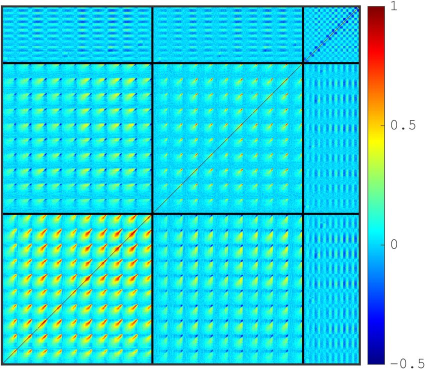
lensing cosmic shear analyses (Joudaki et al. 2017; Chang et al. 2019; Fig. 5 shows the resulting matrix, normalized to unity of the diagonal,
Joudaki et al. 2020; Asgari et al. 2021; Joachimi et al. 2021).17 It √
e.g. r(x, y) = Cov(x, y)/ Cov(x, x) Cov(y, y). Whereas the ξ +
turns out that these approaches do not make too much of an impact for block shows the highest level of correlation, the off-diagonal blocks
current cosmic shear data. Moreover, it is not our primary goal here are mostly uncorrelated, which is promising for the prospect of
to optimise these choices, as we are rather interested in establishing learning additional information from the joint analysis.
our simulation-based inference method as being robust, accurate,
and flexible. We therefore opted for an overall analysis pipeline that
maximally resembles that of the fiducial DES-Y1 cosmic shear data, 3.5 Peak function emulator
and leave some additional tuning for future work.
The peak count statistics measured from the Cosmology training set
Aside from a different choice of n(z) calibration (see Section 2.1),
(shown in Fig. 4 with the coloured histograms) is computed at 26
the key differences between our current pipeline and that of T18
points in a wide four-dimensional volume. From these we train a
are the impossibility of ours to vary and marginalize over the other
Gaussian Process Regression (GPR) emulator that can model the
cosmological parameters – the power spectrum tilt parameter
ns ,
peak function given an input set of cosmological parameters [m ,
the baryon density b and the sum of neutrino mass mν . These
S8 , h, w0 ] at any point within the training volume. Directly adapted
would require more light-cone simulations such as the Mira-Titan
from the public cosmo-SLICS emulator18 described in appendix A
(Heitmann et al. 2016) or the MassiveNuS (Liu et al. 2018) that are not
of HD19, we train our GPR emulator on the individual elements of
folded in our training set at the moment but form a natural extension
the Npeaks data vector, first optimizing the hyper-parameters from an
to this work. Also missing is a cosmology-dependent model for the
MCMC analysis that includes 200 training restarts, then ‘freezing’
effect of intrinsic alignment, which could be necessary in future
the emulator once the best-fitting solution has been found. As de-
analyses.
scribed in HD19, the training can also involve a PCA decomposition
and a measurement error; we include the former but find that the
modelling is more accurate without the latter.
3.4 Covariance matrix
We evaluate the accuracy of the emulator from a leave-one-out
The covariance matrix is a central ingredient to our cosmological cross-validation test: the emulator is trained on all but one of the
inference as it describes the level of correlation between different training nodes, then generates a prediction of the peak function at
elements of our data vector, and its inverse directly enters in the the removed cosmology, which is finally compared with the actual
evaluation of the likelihood. In our analysis, it is estimated from the measurement. This test is performed for all nodes and provides
Covariance training set, which is based on 124 independent light- an upper bound on the interpolation error, since in this case the
cones, each replicated on to the 19 survey tiles such as to fully cover distance between the evaluation point and all other training nodes
the DES-Y1 footprint. For each of these survey realizations, we is significantly larger than if all points had been present. Moreover,
further generate 10 shape noise realizations by randomly rotating the many of these points lie at the edge of the training volume, hence
ellipticity measurements from the data, which increases the number removing them for this test requires the emulator to extrapolate
of pseudo-independent realizations to Nsim = 1240 and is largely from the other points, which is significantly less accurate than the
enough for the current analysis. interpolation that is normally performed. As discussed in HD19,
the node at the fiducial cosmology was added by hand close to the
centre of the wCDM Latin hypercube, hence the cross-validation test
17 In performed at that single CDM point is more representative of the
particular, Joachimi et al. (2021) demonstrates that reporting the
projected maximum likelihood value and the associated confidence interval actual emulator’s accuracy.
can introduce biases when collapsing a high-dimensional hyper-volume into The results from this accuracy test are presented in Fig. 6,
a one-dimensional space. Instead, it is argued therein that a more accurate 1D again colour coded with S8 . We achieve sub-per cent interpolation
inference is obtained by reporting the multivariate MAP distribution, along
with a credible interval calculated using the projected joint highest posterior
density (PJ-HPD) of the full likelihood. 18 github.com/benjamingiblin/GPR Emulator/
MNRAS 506, 1623–1650 (2021)You can also read