Climate resilient water management in Wellington, New Zealand Nigel Taptiklis NZCCRI 2011 report 09
←
→
Page content transcription
If your browser does not render page correctly, please read the page content below
Climate resilient water management in Wellington,
New Zealand

        Nigel Taptiklis

        NZCCRI 2011 report 09
        October 2011

        The New Zealand Climate Change Research Institute
        Victoria University of Wellington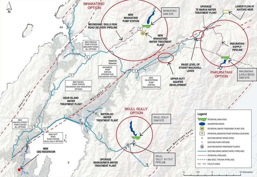
The New Zealand Climate Change Research Institute
School of Geography, Environment and Earth Sciences
Victoria University of Wellington
PO Box 600
Wellington
New Zealand

Contact:           Liz Thomas
Phone:             (04) 463 5507
Email:             liz.thomas@vuw.ac.nz

Acknowledgements
This research was funded by the Foundation for Research, Science and Technology under contract
VICX0805 Community Vulnerability and Resilience. This research was supervised by Associate
Professor Ralph Chapman of the School of Geography, Environment and Earth Sciences at Victoria
University of Wellington, and Dr Andy Reisinger CCRI (for the first seven months). Judy Lawrence
provided significant oversight and editorial advice for this report. Andrew Tait at the National
Institute of Water and Atmospheric Research (NIWA) organised the climate and hydrological data,
which Geoff Williams at Greater Wellington Regional Council (GWRC) used in GWRC’s sustainable
yield model to produce data for this case study. Systems modeller Jason Markham provided
technical and methodological support for the participatory modelling workshops. This research
could not have been completed without the ongoing support and contributions from Professor
Martin Manning and the CCRI team, NIWA, and GWRC. The researcher would like to thank the
participants who shared their views and experiences in the interviews and workshops conducted for
this study.

Contract: E1307

 Vulnerability, Resilience, and Adaptation Objective 2 reports, October 2011
 NZCCRI-2011-01       Synthesis: Community vulnerability, resilience and adaptation to climate change in New Zealand
 NZCCRI-2011-02       Vulnerability and adaptation to increased flood risk with climate change—Hutt Valley summary (Case
                      study: Flooding)
 NZCCRI-2011-03       The potential effects of climate change on flood frequency in the Hutt River (SGEES client report)
                      (Case study: Flooding)
 NZCCRI-2011-04       Potential flooding and inundation on the Hutt River (SGEES client report) (Case study: Flooding)
 NZCCRI-2011-05       RiskScape: Flood-fragility methodology (NIWA client report) (Case study: Flooding)
 NZCCRI-2011-06       Vulnerability and adaptation to increased flood risk with climate change—Hutt Valley household
                      survey (Case study: Flooding)
 NZCCRI-2011-07       Perspectives on flood-risk management under climate change—implications for local government
                      decision making (Case study: Flooding)
 NZCCRI-2011-08       Vulnerability and adaptation to sea-level rise in Auckland, New Zealand (Case study: Sea-level rise)
 NZCCRI-2011-09       Climate resilient water management in Wellington, New Zealand (Case study: Water security)
All reports available on the NZCCRI website: http://www.victoria.ac.nz/climate-change/reports

                                                             ii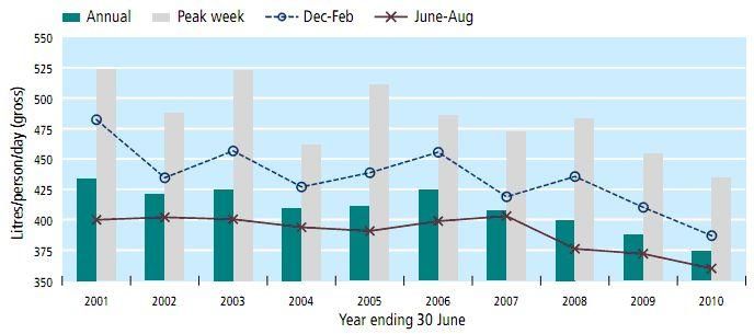
New Zealand Climate Change Research Institute

Contents
Executive summary .......................................................................................................................................... 1

1.            Introduction and overview ............................................................................................................... 5
     1.1.      Background ..................................................................................................................................... 5

     1.2.      Research purpose ............................................................................................................................ 5
     1.3.      Research questions .......................................................................................................................... 6
     1.4.      Research framework ........................................................................................................................ 6

2.            Water management: A multi-dimensional system challenge ............................................................. 9

     2.1.      Post-normal science and systems thinking ....................................................................................... 9
     2.2.      Wellington’s water management context....................................................................................... 10

3.            Climate change and water supply and demand drivers ................................................................... 13
     3.1.      Methodology ................................................................................................................................. 13

     3.2.      Results........................................................................................................................................... 15
     3.3.      Discussion...................................................................................................................................... 24
     3.4.      Summary ....................................................................................................................................... 26

4.            Adaptive capacity and resilience to water shortages ....................................................................... 27

     4.1.      Methodology ................................................................................................................................. 27
     4.2.      Exposure, sensitivity, and response pathways ................................................................................ 29
     4.3.      Adaptive capacity and transformation............................................................................................ 32
     4.4.      Local contextual factors ................................................................................................................. 34

     4.5.      Discussion...................................................................................................................................... 43
     4.6.      Summary ....................................................................................................................................... 48

5.            Conclusion: Resilience and urban water management .................................................................... 51
     5.1.      Resilience and vulnerability............................................................................................................ 51

     5.2.      Participatory adaptive management .............................................................................................. 51
     5.3.      Wellington water management...................................................................................................... 52

6.            References ..................................................................................................................................... 54

7.            Appendix 1: Systems-thinking tools ............................................................................................... 61

     7.1.      Limitations..................................................................................................................................... 62

                                                                                iii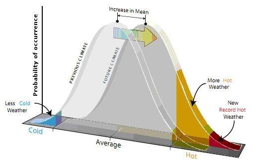
iv

List of figures and tables
Figure 1.    Vulnerability and its components (Allen Consulting Group 2005) ................................................. 7
Figure 2.    The ‘post-normal science diagram’ showing three types of problem-solving strategies
             (Ravetz 2006, Funtowicz and Ravetz, 1993). ................................................................................. 9
Figure 3.    Greater Wellington Regional Council water supply network (GW 2010). ..................................... 11
Figure 4.    Average daily demand (Avg day) and resident population (serviced by water reticulation
             network) for Wellington 1985 to 2010 (Graph updated from GW 2008). .................................... 12

Figure 5.    Global average temperature increase relative to pre-industrial times for the A2 ‘high
             carbon world’ and the low-carbon ‘Rapidly decarbonising world’ scenarios (relative to 1860–
             1899). The vertical bars to the right indicate the likely range (66% probability) for each scenario
             during 2090-2099 (Reisinger et al. 2010). The grey area shows the range of temperatures
             simulated for the twentieth and twenty-first centuries, indicating that due to uncertainties in the
             climate system, the ‘high carbon’ scenario is not an ‘upper end’. ............................................... 14
Figure 6.    Relationships between PCD, PAW, TSD, and net-flow with their respective daily average current
             values (data from 2009 / 2010, PCD based on 5-year average). .................................................. 14

Figure 7.    Average daily supply (PAW) -1 standard deviation, and average daily demand (TSD) + 1 standard
             deviation in ML / day, from December to March under present climate variability. .................... 16

Figure 8.    Average daily supply (PAW) 2040 and 2090 by month and IPCC A2, B1 and low-carbon
             scenarios (Mod 12). ................................................................................................................... 16
Figure 9.    Average PCD 2040 and 2090 by month and IPCC A2, B1, and low-carbon scenarios (Mod 12). .... 17
Figure 10.   Average daily supply (PAW) -1 standard deviation, and average daily flow demanded (TSD)
             + 1 standard deviation in ML / day, from December to March under climate variability for 2040
             A2 with population growth (Mod 12). ........................................................................................ 17
Figure 11.   Running net-flows for 2040 A2, 2090 A2, and low-carbon scenarios for projected population
             growth with average aggregate per capita demand equivalent to 404 L / day. The boxes show the
             first and third quartiles and median. Whiskers go to the 2nd and 98th percentiles, and the largest
             and smallest data points are marked as ‘outliers’ with black crosses. The means are shown with
             pink crosses. .............................................................................................................................. 18
Figure 12.   Figure 3.8: Running net-flows with no population increase for 2040 A2, and 2090 A2 and low-
             carbon scenarios........................................................................................................................ 19
Figure 13.   Figure 3.9: Declining PCD in Wellington 2001–2010 (Capacity 2010). .......................................... 20
Figure 14.   Running net-flows for scenarios 2040 and 2090 using both the A2 and low-carbon scenarios, for
             projected population growth with average aggregate per capita demand equivalent to 303 L /
             day. ........................................................................................................................................... 21

Figure 15.   Running net-flows for 2040 A2, 2090 A2, and low-carbon scenarios with average aggregate PCD
             equivalent to 300 L / day and no population growth. ................................................................. 22

Figure 16.   300-day sequence of the largest deficit event generated for 2010 with PCD of 404 L / day, and
             2040 with PCD of 303 L / day scenarios. The green line indicates a ‘minimum deficit’ with
             substantial and early demand management (A2 mod12, 80 day running-net). The miub (aqua)
             and mpi (orange) projections show the model range at the peak of the deficit. .......................... 23

                                                                           iv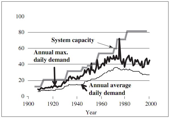
New Zealand Climate Change Research Institute

Figure 17.   Climate change and increased risk of extremes. With regard to temperature, an increase in mean
             temperature within reference climate conditions results in a significant increase in the
             occurrence of hot weather, including record hot weather (Reisinger et al. 2010). ....................... 24

Figure 18.   Stakeholder scales and domains. Adaptation of schematic presented by Mortimer (2010). ........ 28
Figure 19.   Response pathway diagram showing influence of key responses (green) on system variables
             (blue) to reduce community exposure and sensitivity (yellow) to water shortages due to
             increasing climate change and population.................................................................................. 29

Figure 20.   Structure diagram demonstrating socio-ecological system feedbacks resulting from response
             pathways (green) with regard to exposure and sensitivity to water shortages. ‘Capacity’ is a
             measure of consumption to supply, e.g. number of days of storage or percentage of supply
             consumed at peak consumption. ............................................................................................... 30

Figure 21.   ‘Behaviour over time’ graph demonstrating implications for exposure and sensitivity to water
             shortages with and without water conservation as the primary response pathway..................... 31

Figure 22.   Structure diagram demonstrating feedback differences between ‘supply management’ (B1) and
             ‘demand management’ B2. The water security standard serves as a proxy for exposure, while Per
             Capita Demand (PCD) could be used as a proxy measure of sensitivity. ...................................... 32
Figure 23.   Schematic of a successful example of transformation towards adaptive co-management (Folke et
             al. 2005). ................................................................................................................................... 33
Figure 24.   Feedback structures and system interactions between demand-side intervention options (green)
             and the target variables ‘water conservation’ and 'consumption' (yellow). R3, R5, and R8 indicate
             key structures that influence adaptive capacity. ......................................................................... 34

Figure 25.   Augmentation and upgrade options, plus Wellington Fault location (GW 2008b). ....................... 41
Figure 26.   Comparison of unit costs for various demand management options including rainwater (blue
             circle) in an Australian context (Turner et al. 2009). ................................................................... 42
Figure 27.   Responding to an extreme event based on historical trends led to an increasing and expensive
             gap between capacity and consumption for a big city in Switzerland (adapted from Pahl-Wostl
             2005). ........................................................................................................................................ 44

Figure 28.   The adaptive management cycle. ............................................................................................... 47
Figure 29.   Simple structure diagrams showing balancing and reinforcing feedback structures. In general, an
             increase in price leads to a decrease in consumption, which leads to a decrease in price, and an
             increase in consumption (Loop B1). Loop R1 indicates that an increase in income enables an
             increase in investment, thereby providing an increase in income, therefore allowing an increase
             in investment............................................................................................................................. 61
Figure 30.   Behaviour over time graph for the variables 'Price' and 'Income' above...................................... 62

Table 1.     Water savings and changes in consumption and population to 2025 with 1.5% annual demand
             reduction and 1% population growth. Projections for the ‘2040 scenario’ column are shown in
             Figures 14 and 15. ..................................................................................................................... 20

                                                                           v
vi
List of acronyms
ASP Annual shortfall probability
BOT Behaviour over time
CLD Causal loop diagram
CO2 Carbon dioxide
CPR Common property resource
GWRC Greater Wellington Regional Council
GWW Greater Wellington Water
HCC Hutt City Council
IPCC Intergovernmental Panel on Climate Change
ML Million litres
NGO Non-governmental organisation
PAW Potentially available water
PCC Porirua City Council
PCD Per capita demand
PCE Parliamentary Commission for the Environment
RMA Resource Management Act 1991
SYM Sustainable yield model
TSD Total system demand
WCC Wellington City Council
viNew Zealand Climate Change Research Institute
Executive summary
A confluence of factors, including population growth and climate change, poses significant
challenges to the sustainability of cities worldwide. In addition, climate change adaptation is now a
necessity since past and present carbon dioxide (CO2) emissions represent a commitment to further
warming for the next few decades (Jones 2010, IPCC 2007b).
Research purpose
This report sets out the findings of the Wellington case study on urban water supply management,
which is one of three case studies that form Objective 2 of the collaborative, interdisciplinary
research project on Community Vulnerability, Resilience and Adaptation to the impacts of climate
change. The project is led by Victoria University and funded by the Foundation for Research, Science
and Technology (FRST)1.
This case study focuses on water supply management for the four cities of Wellington, Porirua,
Lower Hutt, and Upper Hutt, which are serviced by the one reticulated network. The aim of this
research is to gain a detailed understanding of the factors influencing water use and management in
Wellington, and how specific response options could affect future community and institutional
adaptive capacity, and increase or decrease resilience to water shortages.
This case study into climate change adaptation and urban water management used systems-
thinking, resilience, and complex systems science approaches. Such an approach is indicated when
water management is seen as a complex, multi-dimensional system challenge. For example, water
management requires decisions on long-term infrastructure projects that are highly dependent on
human behaviour and actions (past and future), environmental parameters, and on long-term
climate change. These interacting human, physical, and biological factors can be seen as
components of a coupled socio-ecological system2. Decision makers involved in such issues can
expect to encounter a plurality of objectives, politics, and legacies where ‘the facts are uncertain,
values in dispute, stakes high and decisions urgent’ (Funtowicz and Ravetz 1991).
1
FRST was merged in February 2011 with the Ministry of Research, Science and Technology (MoRST) to form
the Ministry of Science and Innovation (MSI), which is responsible for the policy and investment functions of
both those agencies.
2
A socio-ecological systems view sees human communities and ecological systems as coupled, integrated
systems—i.e. human societies are a part of the biosphere and are embedded within ecological systems (Folke
et al. 2002).
1Research questions
This case study was structured around the following research question.
What factors might lead Wellington as a community to a pathway of greater adaptive capacity and
resilience, and what vulnerabilities might lead to insufficient adaptation or even maladaptation 3?
This question was broken down into the following parts.
1. How might climate change trends interact with water supply-and-demand factors to create
water security and management issues for Wellington?
2. What are the implications of primary response pathways and options (including governance and
management approaches) for community resilience and adaptive capacity?
3. How might Wellington as a community adapt to water shocks or constraints, and what might
impede or facilitate adaptation?
Research findings
Wellington’s present water supply capacity is sufficient to meet increased demand due to
population growth and climate change in all but the driest years to 2090
Climate change and water-demand scenarios for 2040 and 2090 were generated using Greater
Wellington Regional Council’s (GWRC) ‘sustainable yield’ model (SYM) and downscaled climate
model data. This data was used to provide a general understanding of trends and dynamics over
time, by looking at interacting supply and demand drivers. A general analysis indicates that, with a
20 percent reduction in per capita demand and additional storage, Wellington’s present supply
capacity is sufficient to meet increased demand due to climate change and population growth, and
cope with decreased supply due to climate change in all but the driest years to 2090.
An approach focused primarily on supply management could increase vulnerability to water
shortages
Dry conditions concurrently decrease supply and increase demand for water, and climate change is
projected to bring increasing frequency and severity of drought to some regions of New Zealand
(Hennessy et al. 2007, IPCC 2007b). As dry conditions become more frequent and severe, the risk of
water shortages is exacerbated, which also increases the storage and supply capacity requirements
for the water system. However, local-level climate projections under-represent climate variability,
due to averaging within climate models. This then flows onto probability-based calculations for
system capacity requirements which will also underestimate variability and extremes. Moreover,
since it is not possible to rule out a water shortage for a coming summer, and since responding to a
drought requires demand-management measures be actioned as early as possible, management
approaches that encourage sensible (moderated) summer water use are needed every summer.
Meanwhile, an approach that is primarily focused on supply management could increase
vulnerability to water shortages.
3
Maladaptation is defined as ‘action taken ostensibly to avoid or reduce vulnerability to climate change that
impacts adversely on, or increases the vulnerability of other systems, sectors or social groups’ (Barnett and
O’Neill 2010). ‘Other groups’ could also include future citizens.
2New Zealand Climate Change Research Institute
Wellington’s water intensity is declining, in spite of a lack of incentives and signals
Resilience and response option selection, semi-structured interviews, and a systems modelling
workshop were conducted to gain an understanding of the local context for adaptation. Despite a
lack of incentives and signals, Wellington’s water intensity is currently in decline. There is also
considerable potential to further reduce Wellington’s water intensity, with potentially large
inefficiencies in Wellington’s metered CBD, and the general absence of residential water metering.
Standards, regulation, and financial and environmental concerns drive water conservation efforts at
the local government level, while political dynamics and a perceived low priority for water
conservation can act as barriers.
A pilot project could facilitate community collaboration and participation in water management
Analysis of workshops, interviews and literature indicates that enhancing community adaptive
capacity to increase resilience to water shortages requires social learning, a process that can be
facilitated through participative and collaborative involvement in water management. Designing a
pilot project to facilitate community collaboration and participation in water management is
recommended to initiate cross-scale experimentation, learning, and adaptation—from end users to
water managers and government decision makers.
3New Zealand Climate Change Research Institute
1. Introduction and overview
1.1. Background
Adapting to a changing climate is a necessity since past and present anthropogenic greenhouse gas
emissions represent a commitment to further warming for the next few decades (Jones 2010, IPCC
2007b). In some regions of New Zealand, particularly northern and eastern areas, the frequency and
severity of droughts is projected to increase over time due to climate change (Hennessy et al. 2007,
IPCC 2007b). Dry conditions affect both supply and demand for water. In general, increased
frequency and severity of drought will increase the overall variability of water supply and demand
that must be ‘managed’, in particular the risk of water shortages.
The Intergovernmental Panel on Climate Change (IPCC) (IPCC, 2007b, p.19) highlight that ‘effective
adaptation measures are highly dependent on specific geographical and climate risk factors as well
as institutional, political and financial constraints’. In addition, climate change adaptation measures
are generally not undertaken in response to climate change alone, but ‘tend to be on-going
processes, reflecting many factors or stresses, rather than discrete measures to address climate
change specifically’ (Adger et al. 2007, p.720). From a systems perspective, climate change
adaptation can be seen as part of an interconnected system of social, economic, and physical system
components, each changing over time in response to internal and external drivers.
In a complex interconnected system, the decisions communities make will be dependent on current
and previous events and decisions, present and projected trends, and on existing structures and
approaches. Such decisions will have wider social, economic, cultural, and ecological implications,
including for a community’s own resilience and sustainability.
1.2. Research purpose
This report sets out the findings of the Wellington case study on urban water supply management,
which is one of three case studies that form Objective 2 of the collaborative, interdisciplinary
research project on Community Vulnerability, Resilience and Adaptation to the impacts of climate
change. The project is led by Victoria University and funded by the Foundation for Research, Science
and Technology (FRST)4.
This case study focuses on water supply management for the four cities of Wellington, Porirua,
Lower Hutt, and Upper Hutt, which are serviced by the one reticulated network. The aim of this
research is to gain a detailed understanding of the factors influencing water use and management in
Wellington, and how specific response options could affect future community and institutional
adaptive capacity, and increase or decrease resilience to water shortages.
4
FRST was merged in February 2011 with the Ministry of Research, Science and Technology (MoRST) to form
the Ministry of Science and Innovation (MSI), which is responsible for the policy and investment functions of
both those agencies.
51.3. Research questions
This case study was structured around the following research question.
What factors might lead Wellington as a community to a pathway of greater adaptive capacity and
resilience, and what vulnerabilities might lead to insufficient adaptation or even maladaptation?
This question was broken down into the following parts.
1. How might climate change trends interact with water supply-and-demand factors to create
water security and management issues for Wellington?
2. What are the implications of primary response pathways and options (including governance and
management approaches) for community resilience and adaptive capacity?
3. How might Wellington as a community adapt to water shocks or constraints, and what might
impede or facilitate adaptation?
1.4. Research framework
A resilience / systems perspective was used as a research framework to provide insights on shifting
policy responses away from the present control-orientated approaches that presume a stable
system state, to ‘managing the capacity of social-ecological systems5 to cope with, adapt to, and
shape change’ (Folke et al. 2002, p.4).
1.4.1. Resilience
Resilience is the ability of a system to absorb disturbances while retaining the same basic structure,
ways of functioning, and self-organisation (IPCC 2007). Key aspects of resilience are diversity,
modularity (division and separation of system components), and redundancy (overlapping functions)
(Walker 2009).
1.4.2. Vulnerability
Identifying vulnerability, through the use of resilience principles, provides an efficient framework for
assessing resilience, i.e. by asking in which parts of the system is there little or no diversity,
modularity, or redundancy (Walker 2009).
Vulnerability can be viewed through a framework consisting of exposure, sensitivity, and adaptive
capacity (Adger 2006). The following schematic illustrates how these components can be related
(Fig. 1). In this schematic, policy interventions aiming to reduce vulnerability (to increase resilience)
can either reduce exposure or sensitivity or increase adaptive capacity. Vulnerability is defined by
the IPCC (IPCC, 2007) as:
‘[T]he degree to which a system is susceptible to, and unable to cope with, adverse effects of climate
change, including climate variability and extremes. Vulnerability is a function of the character,
5
A socio-ecological systems view sees human communities and ecological systems as coupled, integrated
systems; i.e. human societies are a part of the biosphere, and are embedded within ecological systems (Folke
et al. 2002).
6New Zealand Climate Change Research Institute
magnitude, and rate of climate change and variation to which a system is exposed, its sensitivity, and
its adaptive capacity.’
Figure 1. Vulnerability and its components (Allen Consulting Group 2005)
1.4.3. Adaptive capacity
Adaptive capacity describes the ability of a system to adapt to climate change to moderate potential
damages, make use of opportunities, or cope with adverse impacts (IPCC 2007). Climate change
adaptation measures are not generally undertaken in response to climate change alone and ’tend to
be on-going processes, reflecting many factors or stresses, rather than discrete measures to address
climate change specifically’ (Adger et al. 2007). Adaptability in a socio-ecological system is the
capacity of actors in that system to manage resilience (Walker et al. 2004).
Holling (1996, 1973) makes a distinction between a traditional view of resilience and a more
dynamic approach. Holling characterises the traditional view as engineering resilience, a property
measurable by the system’s resistance to disturbance and its speed of return to equilibrium (return
time). By contrast, Holling’s second definition of ecological resilience is a more dynamic concept,
‘where the natural state of the system is one of change rather than of equilibrium’ (Nelson et al.
2007, p.398), and where multiple stable states are possible. From this perspective, return time is an
insufficient measure of resilience since there are many other ways for a system to fail, other than fail
to return to its previous state or to retain previous functions (Walker et al. 2004).
1.4.4. Transformability
For a socio-ecological system, a dynamic view of resilience also acknowledges that a community
requires the flexibility to transform itself (Walker et al. 2004), for example, to avoid becoming locked
into an undesirable pathway. Transformability is ‘the capacity to create a fundamentally new system
when ecological, economic, or social (including political) conditions make the existing system
untenable’ (Walker et al. 2004). A narrow view of resilience can be detrimental, for example
increasing the resilience of a particular part of a system to specific disturbances can reduce overall
resilience (Folke et al. 2010).
7New Zealand Climate Change Research Institute
2. Water management: A multi-dimensional system
challenge
Water management requires decisions on long-term infrastructure projects which are highly
dependent on human behaviour and actions (past and future), and on long-term climate change.
Moreover, a confluence of interacting factors including population growth, climate change, resource
constraints, and legacy effects now present water managers with greater complexity and uncertainty
for planning and decision making. These interacting human, physical, and biological factors can be
seen as components of a coupled socio-ecological system, in which water management becomes a
complex, multi-dimensional system challenge.
2.1. Post-normal science and systems thinking
This case study uses the concepts outlined in Section 1.4, in conjunction with post-normal science
and systems-thinking approaches. A post-normal science approach is indicated where both decision
stakes and system uncertainties are high (Fig. 2), while the use of systems thinking acknowledges the
complexity and interconnectedness of human and natural resource systems.
Figure 2. The ‘post-normal science diagram’ showing three types of problem-solving strategies (Ravetz 2006,
Funtowicz and Ravetz, 1993).
System uncertainties in relation to water management and climate change in Wellington include the
effects of sea-level rise on the Waiwhetu Aquifer (Ibbitt and Mullan 2007), the interplay of water
consumption and population trends (e.g. Fig. 27), the rate and magnitude of climate change, and the
resulting impacts at a local level (Jones 2010). Decision stakes become particularly high during and in
response to a water shortage, and in complex systems the full implications of such decisions are
unknowable (Rittel and Webber 1973). Decision makers involved in such issues can expect to
encounter a plurality of objectives, politics, and legacies, where ‘the facts are uncertain, values in
9dispute, stakes high and decisions urgent’ (Funtowicz and Ravetz 1991). Such issues are also
characterised as ‘wicked’ problems (Rittel and Webber 1973).
A primary element of a post-normal science inquiry is the full involvement of an ‘extended peer
community’ consisting of stakeholders representing ‘multiple legitimate perspectives’ (Ravetz 2006,
Saloranta 2001). The extended peer community takes part in the problem-solving process by
introducing ‘extended facts’ into the dialogue, including personal or anecdotal experiences to enable
a richer picture of the issue to emerge (Saloranta 2001).
‘An extended peer community is at the heart of post-normal science, and not some afterthought
provided by the benevolence of the authorities’ (Ravetz 2006, p.277).
Where post-normal science seeks to strengthen decision making by incorporating an extended peer
community, getting a diverse group of stakeholders to sufficiently consider other legitimate
perspectives and mental models is a significant challenge. Significant progress was made by
stakeholders in this regard through the Land and Water Forum. A diverse group of stakeholders
participated in the forum, and collaborated to produce a report and recommendations to advise
water management in New Zealand (http://www.landandwater.org.nz).
2.2. Wellington’s water management context
2.2.1. Water sources
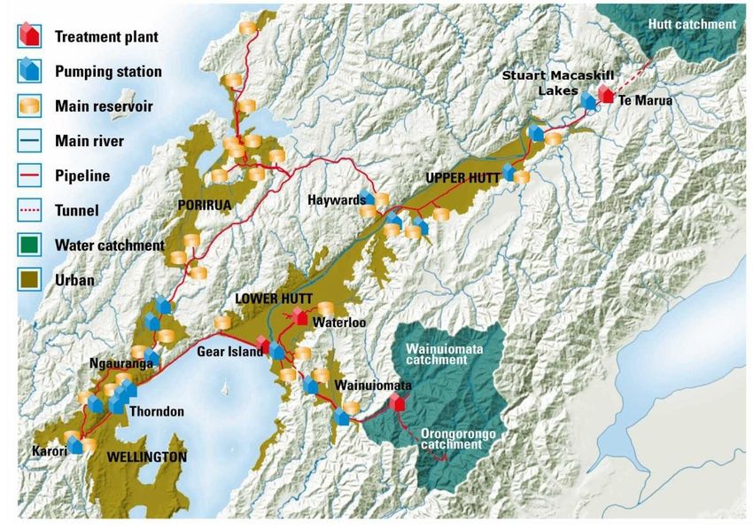
Greater Wellington Water (GWW) treat and distribute ‘bulk’ water to Upper and Lower Hutt,
Porirua, and Wellington cities (Fig. 3). Water is sourced from Waiwhetu Aquifer and the Hutt,
Orongorongo, and Wainuiomata Rivers. On average, 40 percent of Wellington’s water comes from
the aquifer and 60 percent from rivers (MWH 2011). The 3000 ML Stuart Macaskill water storage
lakes6 at Te Marua provide a few weeks of summer storage (MWH 2011) and the Waiwhetu Aquifer7
also acts as a buffer during dry periods (Williams 2011, pers comm). In the year to June 2010, GWW
supplied an average of 145 million litres (ML) of bulk water daily to 390,000 people (GW 2010).
2.2.2. Management
Under the Resource Management Act 1991 (RMA), regional authorities such as GWRC are
responsible for the management, use, and allocation of freshwater resources. The purpose of the
RMA is ‘to promote the sustainable management of natural and physical resources… to meet the
reasonably foreseeable needs of future generations’.
GWW’s purpose reflects this legislative influence: ‘We aim to provide enough high-quality water
each day, now and in the future, to meet the reasonable needs of the people of our region’s four
cities, in a cost-effective and environmentally responsible way’ (GW 2010, p.2).
6
The storage capacity of the Stuart Macaskill Lakes will be 3390 ML once current upgrades are complete (Shaw
and McCarthy 2009).
7
Abstraction occurs at Waterloo and Gear Island, ranging from 20–120 ML / day, and averaging 60 ML / day
(GW 2008c).
10New Zealand Climate Change Research Institute
Capacity Infrastructure Services Limited, a Council-Controlled Trading Organisation owned by
Wellington and Hutt city councils, manages the water infrastructure (including wastewater) and
retailing services for the water that GWRC deliver to Wellington, Hutt, and Upper Hutt city councils.
Porirua City Council manages its own water retailing and infrastructure. Capacity does not own the
water, stormwater, and wastewater assets; set policies; or control rates and user charges—these
roles remain with the councils (Capacity 2010).
‘Capacity Infrastructure Services plans and manages the development and maintenance of the “three
waters”—drinking, storm and waste water. This includes maintaining pipes, managing and
monitoring pump stations and providing advice and information on water conservation to preserve
the Wellington region’s water wealth now and into the future’ (Capacity 2010, p.2).
Figure 3. Greater Wellington Regional Council water supply network (GW 2010).
GWW aims to meet a 2 percent ‘security of supply’ or annual shortfall probability (ASP) standard, i.e.
they aim to meet demand 49 out of 50 years. The security of supply standard represents a level of
service to customers, indicating the frequency with which water restrictions could be imposed in
order to manage demand (WCC 2009)8.
As seen in Figure 4, overall the demand for water has been less than population growth since the
early 1990s. This has been due to factors such as the decline in manufacturing in Wellington since
8
Calculations in 2009 put the standard at 3.9 percent (i.e. a shortage every 26 years on average) (GW 2010).
However, further refinements to the SYM model allowing a greater resolution of analysis indicate that GWW
currently meets its 2 percent standard (WCC 2011).
11the 1980s, urban intensification, infrastructure renewal, and increased public awareness of the need
for water conservation (Williams and McCarthy 2010, pers comm.).
As bulk supplier, GWW charges a water levy to its city council customers based on the relative
percentage of water they use. Wellington City uses the majority (54 percent) of the water, Lower
Hutt (25.3 percent), Porirua (11.7 percent) and Upper Hutt (9.2 percent) (GW 2010). Most
commercial and industrial consumers are metered, though only 1 percent of domestic water users
have meters (GW 2008). In Wellington City, meters are voluntary for residential consumers unless
the residence has a swimming pool greater than 10kL in capacity (WCC, undated). The vast majority
of domestic water users are not charged for water on a user pays basis, but only in relation to their
property value.
Avg day Population
170 400000
165
380000
Resident Population
160
Demand (ML/day)
360000
155
150 340000
145
320000
140
300000
135
130 280000
1985
1986
1987
1988
1989
1990
1991
1992
1993
1994
1995
1996
1997
1998
1999
2000
2001
2002
2003
2004
2005
2006
2007
2008
2009
2010
Year
Figure 4. Average daily demand (Avg day) and resident population (serviced by water reticulation network) for
Wellington 1985 to 2010 (Graph updated from GW 2008).
12New Zealand Climate Change Research Institute
3. Climate change and water supply and demand
drivers
Under the RMA, agencies such as GWRC are required to have particular regard to the effects of
climate change. When considering long-term infrastructure projects this has particular salience. For
example, rainfall to Melbourne’s water supply catchments decreased by about 19 percent in 1997–
2008 compared to 1950–1997, reducing dam inflows by about 40 percent (Jones 2010, p.16).
Regional-scale analysis may indicate the potential for such shifts in operating conditions, which can
then be taken into account when comparing adaptation options and pathways.
This section addresses the first part of the research question by using:
scenarios and projections based on water use in Wellington
climate and hydrological modelling.
3.1. Methodology
GWW uses a computer model; the sustainable yield model (SYM), to enable water managers to
assess the response of the water supply system to changes in infrastructure or operational practice,
as well as changes in climate and demand scenarios. The National Institute of Water and
Atmospheric Research (NIWA) produces supply and demand input files for the SYM using synthetic
daily climatic and water demand sequences that are based directly on historic climate and water
demand data for the four city councils supplied by GWW. NIWA input files were produced for each
of three IPCC emissions scenarios (B1, A1B, A2) for ‘2040’ (averaged over the 2030 to 2049 period 9)
and ‘2090’ (averaged over the 2080 to 2099 period).
The NIWA input files for the SYM are based on a number of relevant regional climate parameters.
These parameters were derived from daily data sequences based on 12 different downscaled
climate model projections as well as a projection based on the average of these 12 models, for each
of the IPCC scenarios for 2040 and 2090. The 12 model average provides a useful general projection
for each scenario, while the individual models themselves provide some indication of a range of
possibilities and the level of ‘agreement’ between models, based on the present level of
understanding of the climate system. A ‘low-carbon’, 2°C stabilisation scenario was also used to
produce input files for the SYM. This scenario was used for 2090 only as the scenarios do not differ
significantly in 2040 (Fig. 5). Further background on using this model and scenario set for New
Zealand is available in Reisinger et al. (2010).
For this analysis, the SYM was used to generate daily potentially available water (PAW) and per
capita demand (PCD) data, providing both supply and demand projections, without storage. Data for
PAW, total system demand (TSD) and PCD were received as SYM outputs from GWW. In addition
‘net-flow’ was calculated by subtracting TSD from PAW. PAW represents daily abstractable volume
in ML from Te Marua, Waterloo, and Wainuiomata water treatment plants combined with existing
9
This 20-year averaging removes ‘much but not all’ of the natural variability as represented by the models
(Resinger et al. 2010).
13consent limits and treatment plant capacities. TSD was calculated by the sum product of the PCD for
each of the eight demand centres and the corresponding population (Williams 2010). PCD is
essentially the aggregated TSD divided by population. The relationship between PCD, PAW, net-flow,
and TSD is shown in Figure 6.
Figure 5. Global average temperature increase relative to pre-industrial times for the A2 ‘high-carbon world’ and the
low-carbon ‘Rapidly decarbonising world’ scenarios (relative to 1860–1899). The vertical bars to the right
indicate the likely range (66% probability) for each scenario during 2090–2099 (Reisinger et al. 2010). The
grey area shows the range of temperatures simulated for the twentieth and twenty-first centuries, indicating
that due to uncertainties in the climate system, the ‘high-carbon’ scenario is not an ‘upper end’.
PAW: Flow available for supply
(60% river 40% aquifer)
PCD: Aggregate
per capita demand
Operates when
242 ML/day PAW >TSD
404 L/day
158 ML/day 84 ML/day
Population Operates when
390,000 TSD>PAW
Net-Flow: Surplus
available for
TSD: flow storage
demanded by (capacity 3390 ML)*
Wellington
*Once current upgrades are complete
Figure 6. Relationships between PCD, PAW, TSD, and net-flow with their respective daily average current values (data
from 2009 / 2010, PCD based on 5-year average).
14New Zealand Climate Change Research Institute
3.1.1. Scenario and model selection
The projected climate parameters for the SYM input files are averaged over a 20-year period. This
averaging is necessary to capture changes in long-term climate versus more short-term variation.
Averaging removes much of the natural variability as represented in the models (Reisinger et al.
2010), yet this variability is a significant consideration at the local scale (Jones 2010). Not
surprisingly, the most likely failing of local-level analysis is that it under-represents climate variability
(Jones 2010). However, many of the impacts of climate change are the result of the ‘surprises’ that
come with extreme weather (Climate Commission 2011) as this is where most of the damage to
communities and assets occurs.
Current trends show IPCC projections to be conservative
Current trends show IPCC projections to be conservative since many variables are tracking at or
above the level of the ‘high’ IPCC projections (Jones 2010). Moreover, past and present emissions
represent a commitment to further warming for the next few decades, yet sufficient mitigation
policy commitments are still lacking, and if / when they arrive will take further time to implement
and have an effect (Jones 2010). Therefore, in selecting specific models and scenarios for analysis for
this case study, a key principle was that prudent adaptation planning needs to take high projections
into account.
Specific details on the approach taken to the selection of projections from the model set, combined
with the supply and demand scenarios used in this case study, is available in NIWA’s urban impacts
toolbox10, along with a detailed discussion on the limitations and uncertainties.
3.2. Results
3.2.1. Potential impacts: Scenario analysis
The seasonal variation of supply and demand can clearly be seen in Figures 7, 8, and 9; demand is
greatest in summer when supply is most restricted. Whilst there is sufficient water to meet
projected demand under average summer conditions, substantial overlap occurs during January,
February, and March at just one standard deviation (Fig. 7).
By 2040, climate change could decrease PAW by 5 percent or 12 ML per day on average for January
and February (Fig. 8). The 12 ML difference is the gap between ‘current’ and the 2040 scenarios for
‘Jan / Feb’.
The projected decrease in PAW between 2040 and 2090 is 5.5 percent, and the projected increase in
PCD from 2010 to 2090 due to climate change is 3 percent (Fig. 9), with a corresponding population
of 467,500 based on current trends. The combined effect of climate change and population growth
on demand would be an average increase of 2.1 ML / day for January and February 2040. With
average PCD modelled at 404 L / day, and the projected population increase, climate change
accounts for 14.1 ML of water for January and February 2040 (i.e. in relation to a reduction in net-
10
See Tool 2.5.3 SYM approach to present-day and future potable water supply and demand.
15flow), or an average daily shortfall of an equivalent volume of water sufficient to supply 35,000
people.
260
240
220
Flow Rate ML/day
200
180
160
140
120
Dec Jan Feb Mar
PAW TSD
Figure 7. Average daily supply (PAW) -1 standard deviation, and average daily demand (TSD) + 1 standard deviation in
ML / day, from December to March under present climate variability.
280
270
260
Flow Rate ML/day
250
240
230
220
210
200
190
180
ug
e
ov
ec
ch
b
il
ct
r
un
Fe
/O
Ap
ar
N
D
/A
/J
n/
pt
M
ly
ay
Ja
Ju
Se
M
2040B1 2040 A2 2090 Low
2090 A2 current
Figure 8. Average daily supply (PAW) 2040 and 2090 by month and IPCC A2, B1 and low-carbon scenarios (Mod 12).
16New Zealand Climate Change Research Institute
470
460
Average demand l/pc/d
450
440
430
420
410
400
390
380
370
ov
ec
ch
g
eb
il
e
ct
pr
Au
un
N
t/O
ar
D
F
A
n/
/J
ly/
M
ep
ay
Ja
Ju
S
M
2040 B1 2040 A2 2090 Low
2090 A2 Current
Figure 9. Average PCD 2040 and 2090 by month and IPCC A2, B1, and low-carbon scenarios (Mod 12).
260
240
Flow Rate ML/day
220
200
180
160
140
Dec Jan Feb Mar
TSD PAW
Figure 10. Average daily supply (PAW) -1 standard deviation, and average daily flow demanded (TSD) + 1 standard
deviation in ML / day, from December to March under climate variability for 2040 A2 with population growth
(Mod 12).
As shown in Figure 10, when the projected population increase for 2040 is taken into account,
average supply and average demand overlap in February, indicating that even in an average year
storage of surplus water from winter would become essential for supplying water in the summer.
1740000
35000
30000
25000
20000
Net flow ML/year
15000
10000
5000
0
-5000
-10000
-15000
-20000
-25000
2010 2040_A2 2090_A2 2090low
Scenario (running-net miub)
Figure 11. Running net-flows for 2040 A2, 2090 A2, and low-carbon scenarios for projected population growth with
average aggregate per capita demand equivalent to 404 L / day. The boxes show the first and third quartiles
and median. Whiskers go to the 2nd and 98th percentiles, and the largest and smallest data points are
marked as ‘outliers’ with black crosses. The means are shown with pink crosses.
During a drier than average summer, daily demand may easily increase by more than one standard
deviation from the mean with a concurrent decrease in supply. As a dry summer progresses, the
deficit between demand and supply can grow considerably. Figure 11 shows the potential degree of
annual variability for net-flow. As shown in Figure 11, with climate change, population growth and
average PCD at 404 L / day, the mean running net-flow (supply less demand) is below zero for both
the A2 and low-carbon scenarios by 2090. This indicates that even if balanced over a year and with
large amounts of storage, the flow of water available to Wellington from current sources will be
insufficient to meet projected demand. The minimum value for the 2040 box plot is close to zero,
which indicates that even with as much as 20,000 ML of storage capacity to balance supply and
demand flows over a year; there may not be enough water to meet projected demand in a
particularly dry year by 2040.
18New Zealand Climate Change Research Institute
40000
35000
30000
Net-flow ML/year
25000
20000
15000
10000
5000
2010 2040_A2 2090_A2 2090low
Scenario (running-net miub)
Figure 12. Figure 3.1: Running net-flows with no population increase for 2040 A2, and 2090 A2 and low-carbon
scenarios.
Assuming average PCD of 404 L / day; population growth coupled with climate change pushes the
mean running net-flow down by 15,000 ML / year by 2040 and then by another 25,000 ML / year
between 2040 and 2090 (Fig. 11). In Figure 12 the effect of population growth on the running net-
flow has been removed by holding the population constant at 390,000. By holding population
constant, the difference in net-flow shows the relative effect of climate change, with average PCD at
404 L / day. The mean annual net balance is 3144 ML / year less between 2010 and 2040 (equivalent
to the capacity of the Stuart Macaskill storage lakes), and there is a 5850 ML / year difference
between the 2040 and 2090 A2 scenarios (Fig. 12). In percentage terms climate change alone
decreases mean annual net-flow by 10 percent from 2010 to 2040, and by 21 percent from 2040 to
2090.
3.2.2. Potential impacts: Wider considerations
PCD in the SYM model is based on average water consumption of the last 5 years, which is
404 ML / day. However, daily per capita water consumption for Wellington has been decreasing
steadily for both peak and base demand. The average rate of decline has been 3.3 percent per year
over the last 4 years, or 1.5 percent per year averaged over the last 10 years (see Figure 13). While
Wellington’s population has been growing at an average of 1 percent over the last 10 years, demand
has been falling. In total, PCD fell 25 percent between 1990 and 201011.
11
Calculated from data for Fig. 4.
19If the 1.5 percent average annual reduction in per capita demand continues to 2025, along with a
1 percent annual population increase, Wellington’s aggregate consumption of 375 L per capita / day
will shrink to a similar level to Auckland’s (302 L per capita / day; Kenway 2008) by 2025. In addition,
Wellington’s average total daily demand will decrease from 146 ML / day to 135 ML / day (Table 1).
Figure 13. Figure 3.2: Declining PCD in Wellington 2001–2010 (Capacity 2010).
Year 2010 2015 2020 2025 2040
Scenario
Aggregate PCD 374 347 322 298 303
(L / day)
Domestic PCD12 235 218 203 189 191
(L / day)
Population 390,000 410,000 431,000 453,000 467,50013
Annual Average 146 142 139 135 142
Consumption
(ML / day)
Water saving (per 0% 7% 14% 20% 20%14
capita, 2010 baseline)
Table 1. Water savings and changes in consumption and population to 2025 with 1.5% annual demand reduction and
1% population growth. Projections for the ‘2040 scenario’ column are shown in Figures 14 and 15.
12
Sixty-three percent of aggregate PCD
13
Projected population used for the Wellington case study scenarios, equates to an average annual population
increase of 0.6 percent from 2010.
14
Includes 1 percent projected increase in PCD due to climate change
20New Zealand Climate Change Research Institute
Auckland’s current level of water intensity and the calculations in Table 1 show that a reduction to
303 L / day is theoretically feasible by 2025. Figure 14 presents a scenario where average PCD is
reduced to 303 L / day by 2040. The data indicates that with this scenario there is sufficient water
available for storage, enabling projected demand to be met in all but the most extreme summers
under the 2090 A2 climate scenario. By 2040, with population growth, climate change, and a
reduction in average PCD to 303 L / day, the mean annual running net-flow increases relative to
2010 by 2700 ML / year, and then decreases by 19,000 ML / year between 2040 and 2090 for the A2
scenario (Fig. 14).
45000
40000
35000
30000
Net flow ML/year
25000
20000
15000
10000
5000
0
-5000
2010 (PCD 2040_A2 2090_A2 2090low
404L/day) Scenario (running-net miub)
Figure 14. Running net-flows for scenarios 2040 and 2090 using both the A2 and low-carbon scenarios, for projected
population growth with average aggregate per capita demand equivalent to 303 L / day.
In Figure 15, population has been held constant at 390,000 and average PCD is 33 L / day to show
the relative effect of climate change. There is a reduction in average net-flow of 3300 ML / day
between 2010 and 2040, and 5,686 ML / day between 2040 and 2090. The relative contribution of
climate change to the decrease between 2010 and 2040 is 7 percent, and between 2040 and 2090 it
is 13.5 percent.
2155000
50000
45000
Net flow ML/year
40000
35000
30000
25000
20000
2010 (PCD 2040_A2 2090_A2 2090low
303L/day)
Scenario (running-net miub)
Figure 15. Running net-flows for 2040 A2, 2090 A2, and low-carbon scenarios with average aggregate PCD equivalent to
300 L / day and no population growth.
3.2.3. Water shortage dynamics
A water shortage event is the net effect of both supply and demand factors, which includes a range
of variables such as population, intensity of water use, storage capacity, and water supply dynamics
(e.g. aquifer and / or river extraction). Therefore the occurrence frequency of ‘water shortage’
events in the context of an urban water-supply system differs considerably from drought frequency,
which is primarily climate related (i.e. a water shortage may be more or less frequent depending on
water intensity and supply and storage capacity).
Trenberth (2011) suggests that trend plus variability may be useful for understanding extremes. The
2040 and 2090 projections produced as outputs by the SYM indicate the extent of the trend increase
for that point in the future, while a running-net balance can be used to indicate variability. A
scenario with average PCD of 303 L / day was calculated for 2040 (A2 mod12) 15. The net-flow over an
80-day period (80 day running-net, Fig. 16) gives the largest deficit for this scenario: a longer or
shorter duration fails to capture the full extent of the deficit. The 12 model average projection for
the A2 scenario was used to enable a more rigorous analysis of individual events within the data
series.
Two events with deficits of 14,000 to 15,000 ML appear in the data (one per 57.5 years), one of
which is shown in Figure 16. In addition, there were five events with deficits of 12,000 to 14, 000 ML
(one per 23 years), and 10 events with deficits of 10,000 to 12,000 ML (one per 11.5 years). In total
15
I.e. using the IPCC A2 scenario projected by the 12 model average.
22You can also read