Filling the gap between plot and landscape scale - eight years of soil erosion monitoring in 14 adjacent watersheds under soil conservation at ...

Page created by Kathleen Ingram
 
CONTINUE READING
Filling the gap between plot and landscape scale - eight years of soil erosion monitoring in 14 adjacent watersheds under soil conservation at ...
Adv. Geosci., 48, 31–48, 2019
https://doi.org/10.5194/adgeo-48-31-2019
© Author(s) 2019. This work is distributed under
the Creative Commons Attribution 4.0 License.

Filling the gap between plot and landscape scale – eight years of soil
erosion monitoring in 14 adjacent watersheds under soil
conservation at Scheyern, Southern Germany
Peter Fiener1 , Florian Wilken1,2 , and Karl Auerswald3
1 Institut
         für Geographie, Universität Augsburg, Alter Postweg 118, 86159 Augsburg, Germany
2 Departement   Umweltsystemwissenschaften, Universitätstrasse 16, 8092 Zürich, Switzerland
3 Lehrstuhl für Grünlandlehre, Technische Universität München, Alte Akademie 12, 85354 Freising, Germany

Correspondence: Karl Auerswald (auerswald@wzw.tum.de) and Peter Fiener (fiener@geo.uni-augsburg.de)

Received: 26 February 2019 – Revised: 16 June 2019 – Accepted: 21 June 2019 – Published: 11 July 2019

Abstract. Watershed studies are essential for erosion re-       strates the distinct need for long-term monitoring in runoff
search because they embed real agricultural practices, het-     and erosion studies.
erogeneity along the flow path, and realistic field sizes and
layouts. An extensive literature review covering publications
from 1970 to 2018 identified a prominent lack of stud-          1   Introduction
ies, which (i) observed watersheds that are small enough
to address runoff and soil delivery of individual land uses,    Soil erosion, due to arable land use, is a major environmental
(ii) were considerably smaller than erosive rain cells ( <      threat (Montanarella et al., 2016; Pimentel, 2006) negatively
400 ha), (iii) accounted for the episodic nature of erosive     affecting on-site soil properties and leading to substantial off-
rainfall and soil conditions by sufficiently long monitoring    site damage (Pimentel and Burgess, 2013). Assessing soil
time series, (iv) accounted for the topographic, pedological,   erosion under natural rain can either be carried out in plot
agricultural and meteorological variability by measuring at     or watershed scale studies (Fig. 1). Plot studies (Fang et al.,
high spatial and temporal resolution, (v) combined many wa-     2017; Nearing et al., 1999; Smets et al., 2009; Wischmeier,
tersheds to allow comparisons, and (vi) were made available.    1966) prevail in number and usually comprise a large num-
Here we provide such a dataset comprising 8 years of com-       ber of plots that are simultaneously measured to account for
prehensive soil erosion monitoring (e.g. agricultural manage-   comparability. On the other hand, watershed studies usually
ment, rainfall, runoff, sediment delivery). The dataset cov-    focus only on one or very few watersheds.
ers 14 adjoining and partly nested watersheds (sizes 0.8 to        The most prominent plot set-up (the Wischmeier plots;
13.7 ha), which were cultivated following integrated (four      22.1 m long, 1.83 m wide; slope 9 %) were established while
crops) and organic farming (seven crops and grassland) prac-    developing the still most used erosion model, the Universal
tices. Drivers of soil loss and runoff in all watersheds were   Soil Loss Equation (USLE; Wischmeier and Smith, 1960).
determined with high spatial and temporal detail (e.g., soil    Nowadays, data of thousands of plot years of the Wischmeier
properties are available for 156 m2 blocks, rain data with      plot types are available for various regions of the world. The
1 min resolution, agricultural practices and soil cover with    major advantages of plot experiments are that plots are rela-
daily resolution). The long-term runoff and especially the      tively easy to establish, represent a more or less homogenous
sediment delivery data underline the dynamic and episodic       area, and can be compared in paired plots (Nearing et al.,
nature of associated processes, controlled by highly dynamic    1999). The major disadvantage of plots is that they can only
spatial and temporal field conditions (soil properties, man-    assess runoff generation mainly driven by surface sealing,
agement, vegetation cover). On average, the largest 10 % of     while other processes of runoff generation like return flow
events lead to 85.4 % sediment delivery for all monitored wa-   are ignored. Similarly, sheet and partly rill erosion can de-
tersheds. The analysis of the Scheyern dataset clearly demon-   velop on plots while (ephemeral) gullying is neglected. Fur-

Published by Copernicus Publications on behalf of the European Geosciences Union.
Filling the gap between plot and landscape scale - eight years of soil erosion monitoring in 14 adjacent watersheds under soil conservation at ...
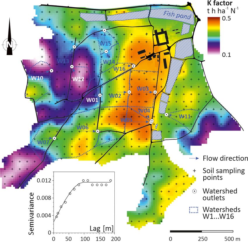
32                                                           P. Fiener et al.: Filling the gap between plot and landscape scale

thermore, heterogeneities along the flow path, variations in        with unique study duration). Furthermore, the majority of
slope, watershed size and soil cover (that may cause highly         studies do not compare more than three watersheds. This
relevant run-on infiltration and sediment settling) are ex-         small number limits a direct comparison and usually does not
cluded in plot experiments. Furthermore, plots typically ex-        allow for an analysis of the influence of spatial variability in
amine a narrow range of dimensions (length, width, length-          watershed properties. Thus, it does not surprise that all wa-
to-width ratio) (Fiener et al., 2011) that differ considerably      tershed studies found in literature report a rather superficial
from dimensions of fields to which the results are mostly sup-      description of topographic, pedologic and agronomic prop-
posed to be applied (Auerswald et al., 2009, Fig. 1).               erties of the watersheds and of the meteorological conditions
   To overcome these problems, a number of watershed scale          during the study period. This becomes evident when com-
monitoring studies were carried out over the last decades           pared to plot studies that at least describe in detail plot mor-
(summarized in Fig. 1). They offer the advantage of suffi-          phology, soil properties and agricultural treatment. The lack
ciently large field sizes to represent: common agricultural         in a detailed description of boundary conditions also impedes
practices, the interaction between neighbouring sites, com-         the combination of data from different studies, although this
plex morphologies and processes like return flow from shal-         would greatly increase the value of such studies. Unfortu-
low ground water or subsurface flow. Thus, watershed stud-          nately, a combination and comparison of different watershed
ies offer large advantages and are an indispensable supple-         studies is impossible because sufficient data are usually not
ment of plot studies. Despite the clear advantages of water-        reported.
shed studies some drawbacks are inherent, which becomes                Here we report about the Scheyern dataset that overcomes
clear from a comparison of such studies performed since             some of the limitations in watershed studies. (i) The dataset
the 1970s (Fig. 1). These studies can be distinguished into         allows for the comparison of a large number of adjacent and
two size categories, (i) those that cover a size range that al-     partly cascading watersheds (14) that are amended by many
lows for a quantification of field or hillslope processes (sizes    plot data under simulated rainfall. (ii) It covers a relatively
< 50 ha) and (ii) those including processes in river systems        long study period (8 years). (iii) The dataset is available and
(> 10 km2 ) to represent storage and release processes of flu-      can be used for comparisons within this dataset, against other
vial systems. However, process scale studies (i) are usu-           datasets or modelling results (for data overview see Table 1).
ally quite short and rarely exceed five years of monitoring         (iv) All watershed sizes are within the range of fields and
(Fig. 1). Taking into account the large temporal and interan-       hillslopes and thus exclude interference of processes along
nual variability of water erosion events (Fischer et al., 2016),    the aquatic flow path. (v) Finally and importantly the data of
this is a serious constraint. Study durations longer than five      soil loss and runoff during erosion events are complemented
years can almost exclusively be found for watershed stud-           by a very detailed set of soil properties (e.g., spatial resolu-
ies of larger scale, although short durations prevail in this       tion of 12.5 m × 12.5 m), weather data (e.g., tipping bucket
size range as well (Fig. 1). An important and unavoidable           rainfall is for some years available up to a spatial resolu-
trade-off associated with large watershed sizes is that in-         tion of 11 km−2 ), agronomic data (all agricultural operations
ternal dynamics within the river system modify the terres-          were recorded), soil cover data and topographic conditions.
trial erosion signal (Auerswald and Geist, 2018; Walling and        Based on this comprehensive dataset, we illustrate the im-
Amos, 1999). Moreover, surface runoff and sediment deliv-           portance of long-term monitoring and of internal temporal
ery is sensitive to the watershed size. Particularly for the up-    dynamics for interpreting watershed deliveries (e.g. the grad-
scaling of processes from plot to landscape scale, the mecha-       ual and asynchronous vegetation cover development on indi-
nistic understanding on field and small watershed scale is es-      vidual fields within a watershed that additionally experience
sential. However, small watershed studies are rare relative to      abrupt changes due to agricultural management and/or may
meso-scale investigations. Furthermore, recent studies have         receive different amounts of erosive rain due to small scale
shown that cells of high intensity rainfall only have a ra-         variability in rainfall depths).
dius of about 2 km based on rain radar measurement (Fis-
cher et al., 2018; Lochbihler et al., 2017). Hence, water-
sheds exceeding the size of 1 km2 are usually only partly           2     Materials and methods
covered by high-intensity rains, while larger watersheds may
respond strongly to medium intensity rains of large spatial         2.1    Test site
extent. Due to the increasing complexity of spatial patterns in
rainfall and internal sediment redistribution and correspond-       The Scheyern Experimental Farm was located about 40 km
ing long-term storage, we restricted our review of watershed        north of Munich, Germany. The test site covered an area of
studies in Fig. 1 to watersheds < 1000 km2 .                        approximately 150 ha (Fig. 2) and is part of the Tertiary hills,
   A further characteristic of watershed studies in compari-        an important agricultural landscape in Central Europe. The
son to plot studies is that usually only few watersheds are         Tertiary sediments are mainly sandy to gravelly, quarzitic,
compared. Numerous monitoring studies have been carried             fluviatile materials of poor fertility. Especially hilltops are of-
out in single watersheds (see all watershed sizes in Fig. 1         ten covered by shallow clayey sediments (either calciferous

Adv. Geosci., 48, 31–48, 2019                                                                    www.adv-geosci.net/48/31/2019/
Filling the gap between plot and landscape scale - eight years of soil erosion monitoring in 14 adjacent watersheds under soil conservation at ...
P. Fiener et al.: Filling the gap between plot and landscape scale                                                                                33

Figure 1. Watershed size and duration of continuous measurements of runoff and sediment delivery for watershed studies taken from literature
since 1970 (black triangles) in comparison with the Scheyern dataset (red triangles). The 99.5 %-range of field sizes in Germany is shaded
in green; the vertical line denotes the average (taken from Auerswald et al., 2018). The approximate range of plot studies with natural rain is
shaded in grey; the vertical and horizontal lines denote the average plot size and the average study duration (taken from Cerdan et al., 2010).
Watershed studies from literature were (Anderson and Potts, 1987; Baker and Johnson, 1979; Beasley, 1979; Beasley et al., 1986; Becht and
Wetzel, 1989; Bingner et al., 1989; Bowie and Bolton, 1972; Brooks et al., 2010; Casali et al., 2008; Chow et al., 1999; Deasy et al., 2011;
Dendy, 1981; Dickinson and Scott, 1975; Didone et al., 2017; Diyabalanage et al., 2017; Duvert et al., 2010; Edwards et al., 1993; Evrard
et al., 2008; Foster et al., 1980; Garcia-Ruiz et al., 2008; Glendell and Brazier, 2014; Grangeon et al., 2017; Hamlett et al., 1983; Hasholt,
1992; Hasholt and Styczen, 1993; Inoubli et al., 2016; Khanbilvardi and Rogowski, 1984; Kimes and Baker, 1979; McDowell et al., 1984;
Mielke, 1985; Mildner and Boyce, 1979; Minella et al., 2018; Monke et al., 1979; Murphree and Mutchler, 1981; Murphree et al., 1985;
Mutchler and Bowie, 1979; Nunes et al., 2016; Onstad et al., 1976; Pieri et al., 2014; Porto et al., 2009; Ramos et al., 2015; Ribolzi et al.,
2017; Schilling et al., 2011; Sheridan et al., 1982; Sherriff et al., 2015; Simanton and Osborn, 1983; Simanton et al., 1980; Simanton and
Renard, 1982; Sith et al., 2017; Sran et al., 2012; Starks et al., 2014; Steegen et al., 2000; Stott et al., 1986; Valentin et al., 2008; Van Oost et
al., 2005; Vongvixay et al., 2018; Walling et al., 2001; Zhang et al., 2015; Zuazo et al., 2012). Note that if watershed data appear in several
studies, only one study was cited here. Data to calculate the decrease in mean rainfall intensity (blue line) with increasing watershed size
were taken from Lochbihler et al. (2017), who analysed the rainfall intensity for the 1000 largest rainfall events of a 9 year period (at 13 to
20 ◦ C; in the Netherlands); for this figure the centre of the rainfall cell is assumed to be located in the middle of the respective watershed.

or not) of former oxbow lakes in the fluviatile Tertiary land-               to 30 %). An intense tachymetric survey was conducted to
scape. Hills were developed during the Pleistocene within                    determine slope angles and watershed boundaries, whereas
these horizontally deposited Tertiary sediments. These hills                 precise elevation was recorded at approximately 4500 po-
are steep on the warm south and west facing slopes due to                    sitions (30 measurements per ha); for details see Warren et
erosion facilitated by the lack of permafrost. The cold east                 al. (2004). Moreover, a 5 m × 5 m LiDAR digital elevation
and north facing slopes had permafrost and solifluction that                 model (DEM) is available. The watershed borders were de-
left gentle slopes. Furthermore the gentle east facing slopes                termined from tachymetric survey and in-situ runoff tracking
received some loess (0 to 2 m), which made them suitable for                 during long-lasting runoff events (snowmelt). This was nec-
cropland, which in turn lead to colluvial soils in toe slope po-             essary as the LiDAR DEM did not properly resolve water-
sitions (Sinowski and Auerswald, 1999). As a result of these                 shed borders due to small scale structures like tillage induced
formation conditions, the research area exhibits a wide range                roughness and grassed ditches along field borders.
of soils, from shallow to deep, from gravelly to sandy to silty                 The climate was temperate humid with a mean annual air
to clayey and a wide range of slope gradients. Well-sorted                   temperature of 8.4 ◦ C during the monitoring phase from 1994
textures dominate in sediments at greater depths (> 30 cm)                   to 2001. The average precipitation was 804 mm yr−1 (1994–
while surface soils are poorly sorted and loamy textures dom-                2001) with the highest precipitation occurring from May to
inate (Auerswald et al., 2001). Following the IUSS Working                   July (average maximum 116 mm per month in July) and the
Group WRB (WRB, 2015), soils at the research farm are                        lowest occurring in the winter months (average minimum
classified Haplic Luvisols, Endogleyic or Haplic or Leptic                   33 mm per month in January). The mean annual erosivity was
Cambisols, Gleyic or Haplic Fluvisols, Mollic Gleysols.                      97 N h−1 yr−1 (Auerswald et al., 2019a).
   The elevation ranged from 448 to 497 m above sea level                       At the research farm, two types of farming systems (con-
with a mean slope of 10.1 % (±6.1 %). Slopes facing south                    ventional and organic farming) were established after har-
and east were gentle (approx. 10 %) while in contrast the                    vest in 1992. The border between both farming systems fol-
slopes facing north and west are partly much steeper (up                     lowed the main watershed boundary in order to have only

www.adv-geosci.net/48/31/2019/                                                                                  Adv. Geosci., 48, 31–48, 2019
Filling the gap between plot and landscape scale - eight years of soil erosion monitoring in 14 adjacent watersheds under soil conservation at ...
34                                                                            P. Fiener et al.: Filling the gap between plot and landscape scale

Table 1. Structure of the Scheyern data base. The zip-files (bold) combine all data and meta-data within one topic, with an individual DOI.
Each zip-file contains several csv files with data, shape files (which are zipped) for geographic information and corresponding pdf files
describing the meta-data.

 Structure of data base                                                                                                           Files
 1.   Soil data                                                                                                                   1_SoilData.zip
      https://doi.org/10.13140/RG.2.2.14231.83365 (Auerswald et al., 2019b)                                                       1_SoilData.pdf
      1.1. Soil profile data: The data set contains 15 properties of entire soil profiles determined at 606 locations.            11_SoilProfilData.csv
                                                                                                                                  11_SoilProfilData.pdf
      1.2. Soil horizon data: The data set contains a total of 46 soil properties determined in 2827 horizons from 504 soil       12_SoilHorizonData.csv
      profiles.                                                                                                                   12_SoilHorizonData.pdf
      1.3. Soil block data: The data set contains a total of 30 soil property averages of 9309 contiguous 12.5×12.5 m2 blocks.    13_SoilBlockData.csv
                                                                                                                                  13_SoilBlockData.pdf
      1.4. Soil physical data: The data set contains 29 physical soil properties of 97 soil horizons for 19 benchmark soils.      14_SoilPhysData.csv
                                                                                                                                  14_SoilPhysData.pdf
      1.5. Adsorbed cation composition and clay mineral composition: The data set contains 7 location variables and 18            15_SoilCatMin.csv
      chemical and mineralogical soil properties that were determined in 108 horizons from 19 benchmark soils.                    15_SoilCatMin.pdf
 2.   Topographic data:                                                                                                           2_TopoData.zip
      https://doi.org/10.13140/RG.2.2.32044.51845 (Wilken et al., 2019a)                                                          2_TopoData.pdf
      2.1. Topographic and surface point data in a regular 5 m × 5 m grid. Data comprise elevation, slope, aspect, field and      21_Topo5m.csv
      watershed information.                                                                                                      21_Topo5m.pdf
      2.2. Topographic and surface point data in a regular 12.5 m × 12.5 m. Data comprise elevation, slope, aspect, field and     22_Topo12_5m.csv
      watershed information.                                                                                                      22_Topo12_5m.pdf
 3.   Meteorological data:                                                                                                        3_MeteoData.zip
      https://doi.org/10.13140/RG.2.2.34561.10088 (Wilken et al. 2019b)                                                           3_MeteoData.pdf
      3.1. Meteostation locations: The data set contains the coordinates and elevation of all 13 meteorological and precipita-    31_MeteoStationsLocation.csv
      tion stations, respectively.                                                                                                31_MeteoStationsLocation.pdf
      3.2. Meteorological station data: The data set contains two files (32_MeteostatM01.csv and 32_MeteostatM02.csv) with        32_MeteoStationM01M02.pdf
      hourly data for 13 parameters measured at the two main meteorological stations on the research farm between 1994 and        32_MeteoStationM01.csv
      2001.                                                                                                                       32_MeteoStationM02.csv
      3.3. Triggered precipitation data: Tipping bucket precipitation on minute resolution of 13 precipitation stations for the   33_TrigPcpData.csv
      years 1994–1997 and of two precipitation stations for the years 1998–2002.                                                  33_TrigPcpData.pdf
      3.4. Continuous and corrected minute-by-minute precipitation data of 13 precipitation stations for the years 1994–1997      34_ContStatPcpData.csv
      and of two precipitation stations for the years 1998-2002. Data are derived from 33_TrigPcpData.csv.                        34_ContStatPcpData.pdf
      3.5. Watershed precipitation data: continuous mean minute-by-minute precipitation data calculated for all 14 individual     35_ContWtshPcpData.csv
      watersheds.                                                                                                                 35_ContWtshPcpData.pfd
      3.6. Data sets 3.4 and 3.5 sub-divided into annual packages to reduce individual file size.                                 36_AnnualPcpData.zip
 4.   Land use data:                                                                                                              4_LandUseData.zip
      https://doi.org/10.13140/RG.2.2.26172.49285 (Auerswald et al., 2019d)                                                       4_LandUseData.pdf
      4.1. Land use data. The data set contains two zipped files with the spatial land use information of 1993 (before restruc-   41_LandUseData1993_2001.pdf
      turing the farm) and 1996 (after restructuring the farm) for use within GIS.                                                41_LandUseData1993.zip
                                                                                                                                  41_LandUseData1994_2001.zip
      4.2. Land management data. The data set contains 17 variables of 1734 individual land management activities that            42_CropManagData.csv
      occurred on 21 arable fields.                                                                                               42_CropManagData.pdf
      4.3. Cover and plant height data. Data on daily soil cover by residues and plants and measurements of plant heights on      43_CovData.csv
      ten organically managed fields and on six conventionally managed fields during the years 1993 to 1997.                      43_CovData.pdf
      4.4. Standardized cover and plant height: Data on the mean daily soil cover by residues and plants and mean plant           44_CoverStandard.csv
      heights for an entire year are given for 20 different crops (conventionally or organically grown). The data allow estima-   44_CoverStandard.pdf
      tion of cover and height from the crop type also in years in which no measurements were made.
      4.5. Main crops: The file compiles the main crops and the catch crops grown on each field between 1993 and 2002. The        45_AnnualCrops.csv
      number of the most appropriate standardized cover and plant height is given.                                                45_AnnualCrops.pdf
      4.6. Tillage direction data. The data set contains the raster based tillage direction of all fields during the monitoring   44_TildirData.csv
      period 1994–2002 (148 430 5 × 5 m2 blocks).                                                                                 44_TildirData.pdf
 5.   Runoff and sediment data from 14 watersheds                                                                                 5_RunSediData.zip
      https://doi.org/10.13140/RG.2.2.30786.22729 (Fiener et al., 2019).                                                          5_RunSediData.pdf
      5.1. Watershed data: The data set contains watershed characteristics (51_WatershedData.csv) and vector data for the         51_WatershedData.zip
      location of the 14 watersheds (51_WatershedData.zip).                                                                       51_WatershedData.csv
                                                                                                                                  51_WatershedData.pdf
      5.2. Runoff data: The data set contains continuous event runoff of 14 watersheds from 1994 to 2001.                         52_RunData.csv
                                                                                                                                  52_RunData.pdf
      5.3. Sediment data: The data set contains measured event sediment concentration of 14 watersheds from 1994 to 2001.         53_SediData.csv
                                                                                                                                  53_SediData.pdf
      5.4. Runoff event precipitation data: The data set contains the watershed-specific event precipitation for each of the      54_EventPrecData.csv
      watersheds.                                                                                                                 54_EventPrecData.pdf
      5.5. Pond data: The data set contains information characterizing the retention ponds located at the down slope end of 6     55_PondData.csv
      of the 14 watersheds and gives sediment trapping efficiencies.                                                              55_PondData.pdf

Adv. Geosci., 48, 31–48, 2019                                                                                             www.adv-geosci.net/48/31/2019/
Filling the gap between plot and landscape scale - eight years of soil erosion monitoring in 14 adjacent watersheds under soil conservation at ...
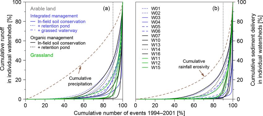
P. Fiener et al.: Filling the gap between plot and landscape scale                                                                                       35

Table 1. Continued.

  Structure of data base                                                                                                            Files
  6.   Runoff and sediment delivery data of 114 rainfall simulation experiments on 57 plots situated in 14 small adjacent           6_RainSimData.zip
       watersheds                                                                                                                   6_RainSimData.pdf
       https://doi.org/10.13140/RG.2.2.27430.78401 (Auerswald et al., 2019c).
       6.1. Plot property data: The data set contains 38 properties of 57 rainfall simulation plots.                                61_PlotData.csv
                                                                                                                                    61_PlotData.pdf
       6.2. Simulation conditions: The data set contains a total of 15 properties determined for 114 rainfall simulation runs (57   62_RunData.csv
       dry runs and 57 very wet runs).                                                                                              62_RunData.pdf
       6.3. Runoff and sediment data: The data set contains a total of 4461 runoff and sediment concentration measurements          63_RoffSedData.csv
       that were made during 114 rainfall simulation runs.                                                                          63_RoffSedData.pdf

                                                                                      fined and continuously applied land use principles of the two
                                                                                      farming systems.
                                                                                         In general, integrated farming and organic farming allow
                                                                                      a wide range of management options. The management of
                                                                                      both farming systems at the research farm aimed to improve
                                                                                      in parallel the economic returns and soil protection (i.e., min-
                                                                                      imizing erosion and soil compaction), water protection (i.e.,
                                                                                      minimizing leaching of agrochemicals), and of biodiversity
                                                                                      enhancement (Auerswald et al., 2000). This multiple-goal
                                                                                      approach required a set of sophisticated and rather unusual
                                                                                      management options like the use of ultra-wide tires on light
                                                                                      tractors or avoiding temporal gaps in soil cover by conse-
                                                                                      quent application of cover crops, catch crops and residues
                                                                                      management. Hence, the management in both systems dif-
                                                                                      fered considerably from what can be found on typical farms
                                                                                      that also apply integrated or organic farming.
                                                                                         The 4-year crop rotation in the integrated farming system
                                                                                      was potato (Solanum tuberosum L.), winter wheat (Triticum
                                                                                      aestivum L.), maize (Zea mays L.), and winter wheat. The
                                                                                      organic farming system had a 7-year crop rotation start-
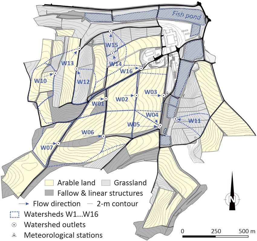
Figure 2. Land use and monitored watersheds at the research farm
(without area for cropping experiments). Numbers ≤ 6 indicate in-                     ing with a grass-clover mixture (typically containing peren-
tegrated management, numbers ≥ 7 indicate organic management.                         nial ryegrass Lolium perenne L., Italian rye-grass Lolium
                                                                                      multiflorum Lam., meadow fescue Festuca pratensis Huds.,
                                                                                      red clover Trifolium pratense L., and white clover Trifolium
                                                                                      repens L.) and followed by potato, winter wheat, winter rye
                                                                                      (Secale cereale L.), white lupine (Lupinus albus L.), and sun-
one system within a certain watershed. One system followed                            flowers (Helianthus annuus L.) (Auerswald et al., 2000). To
the principles of conventional integrated farming (total size:                        meet the rules of nutrient use of the AGOL, the organic farm
46 ha) (not to be confused with the European agriculture or-                          ran a herd of 30 suckler cows with a bull. The cattle were
ganic standard of integrated farming) and the other followed                          grazing the pastures during summer (for details see Auers-
certified organic farming according to the rules of the Ger-                          wald et al., 2010; Schnyder et al., 2010), whereas manure
man Association for Ecological farming (AGOL; total size:                             from the winter stall period was used for fertilizing the or-
68 ha). In general, the organic farming was located in areas                          ganic fields. In the integrated system, maize was produced
with higher soil variability, partly situated at steeper slopes                       that was externally used to feed 49 steers. The slurry from
(mainly grazed) and on less productive soils compared to the                          this herd was applied as manure at the integrated farming
fields of integrated farming. The higher soil variability and                         system.
the steeper slopes required smaller field sizes. Methodologi-                            In order to reduce surface runoff and sediment-bound mat-
cally this was advantageous, because it allowed for the culti-                        ter fluxes, land use and soil management were adapted (see
vation of two fields with the same crop every year despite the                        below) and a number of near-field buffer features were in-
more complex crop rotation. Thus, in both farm types each                             stalled. The latter mainly comprised small retention ponds
crop was replicated in each year. The remaining area of the                           with sub-surface outflows at the downslope end of the water-
farm was used for cropping studies, where treatments were                             sheds W01, W02, W05, W06 and W14 (Fig. 2). The retention
applied that would have been in conflict with the initially de-

www.adv-geosci.net/48/31/2019/                                                                                                Adv. Geosci., 48, 31–48, 2019
Filling the gap between plot and landscape scale - eight years of soil erosion monitoring in 14 adjacent watersheds under soil conservation at ...
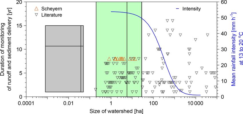
36                                                           P. Fiener et al.: Filling the gap between plot and landscape scale

ponds were designed to retain water for a maximum of three          2.2.2   Soil
days with extreme events (for details see Fiener et al., 2005).
A grassed waterway to prevent ephemeral gullying and re-            A combination of geostatistics and pedotransfer-functions
ducing surface runoff was established in 1993 in the water-         were used to determine the spatial distribution of important
sheds W05 and W06 (for details see Fiener and Auerswald,            soil properties in three dimensions and at high resolution
2003).                                                              (Scheinost et al., 1997). Therefore, soil sampling in a rect-
   The main cropping principle in both farming systems was          angular 50 m × 50 m grid (471 grid nodes) using a machine-
to keep the soil cover high as long as possible, preferably by      auger down to a depth of 1.2 m with a soil core diameter of
growing plants or plant residues where this was not possible.       0.1 m was carried out. In total 2448 soil horizons were sam-
This intended to lower nitrate leaching and erosion but also to     pled and analysed for texture, plant available P and K ac-
increase the input of organic matter into the soil food chain.      cording to Schüller (1969), pH in 0.01 M CaCl, total and
To this end, cover crops were sown and mulch tillage (Kainz,        carbonate C by dry combustion, and total N. Soil texture
1989) was applied in the integrated system while catch crops        was determined for 3 stone fractions and 15 fine earth frac-
were used in the organic system. Also unconventional meth-          tions (Auerswald and Schimmack, 2000). Additionally 19
ods were applied, e.g. sowing mustard (Sinapsis alba L.) into       benchmark soils between the grid nodes were sampled and
potato fields, when the potato leaf cover at the end of the         analysed in more detail. In areas of steep gradients between
growing season decreased due to Phythophtora infestans in-          grid node soils, additional hand augering was applied for soil
fection (Kainz et al., 1997). To prevent soil compaction and        categorization using field methods (for more details regard-
allow reduced tillage, it was necessary using the lightest ma-      ing soil sampling and analysis see Auerswald et al., 2001;
chinery for a given task and using ultra-wide tires on all farm-    Scheinost et al., 1997; Sinowski et al., 1997).
ing machinery. Mouldboard ploughs were used that allowed               All soil data were combined in an extensive geostatisti-
to run with both wheel tracks on the unploughed land, while         cal analysis to interpolate soil properties, e.g. C content and
with the usual mouldboard plough one wheel runs on the sub-         texture, for 12.5 m × 12.5 m grid blocks. For details of the
soil of the furrow and compacts the subsoil; non-inverting          procedure see Scheinost et al. (1997). The geostatistical in-
shallow-depth tillage and stabilization of the soil structure       terpolation scheme was also applied to derive a high resolu-
by increasing biological activity further assisted this concept     tion K factor map, which is used in this study to illustrate
(Auerswald et al., 2000).                                           the richness of the data set and also to underline the impor-
                                                                    tance to account for spatial variability within watersheds to
                                                                    understand differences in hydrological properties. The K fac-
2.2     Data                                                        tor was determined at 544 locations (471 grid nodes and 73
                                                                    points in-between the grid nodes) according to the K factor
                                                                    nomograph (Wischmeier et al., 1971). Bulk soil fractions (in
2.2.1    Soil management and soil cover                             %) of silt (fSi ), very fine sand (fvfSa ), clay (fCl ) and organic
                                                                    matter (fOM ) in the fine earth fraction and the fraction of rock
                                                                    fragments (frf ) were measured; aggregate size class (a) was
Any soil and crop management performed at one of the 23             obtained by visual classification; permeability class (p) was
arable fields was documented by the farm manager. The               estimated from saturated conductivity calculated by using a
available data comprise e.g. sowing date, sowing density,           pedotransfer function that had been developed from mea-
crop type and sowing machinery. Any application of fertilizer       sured saturated conductivities of 737 soil cores taken from
and agro-chemicals was documented including date, machin-           various soils and horizons at the research farm. The range
ery used, type of fertilizer and/or agro-chemical, amounts          of soils exceeded the validity range of the K factor equation
etc.                                                                given by Wischmeier and Smith (1978). In order to avoid
   During the 8 year monitoring period, plant and residue           manual reading of the K factor nomograph for 544 soils, we
cover was measured for 3 1/2 years (January 1993 to                 used the K factor equation by Auerswald et al. (2014) that
April 1997) in all fields. During the vegetation period, mea-       includes all peculiarities of the nomograph, which are not
surements were carried out bi-weekly; during autumn to              included in the simpler equation by Wischmeier and Smith
spring cover was measured monthly and additionally before           (1978). It is a combination of 4 equations; note that there
and after each soil management operation. Measurements              were typing errors in the original publication by Auerswald
were repeated at a minimum of three geodetically defined lo-        et al. (2014); we used the correct equations:
cations within each field. Residue cover and cover of plants
near the surface were measured manually using a meter stick.
Plant height was also determined with a meter stick. Plant
cover of higher plants were derived from photographs taken
around noon from a height up to 4 m (in the case of full-
grown maize) using image analysis (Kaemmerer, 2000).

Adv. Geosci., 48, 31–48, 2019                                                                    www.adv-geosci.net/48/31/2019/
Filling the gap between plot and landscape scale - eight years of soil erosion monitoring in 14 adjacent watersheds under soil conservation at ...
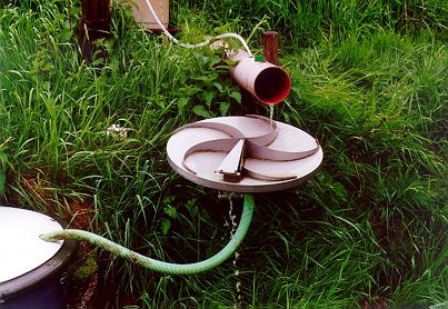
P. Fiener et al.: Filling the gap between plot and landscape scale                                                                 37

K1 = 2.77 × 10⁻⁵ × (fSi+vfSa × (100 − fCl ))1.14
    for fSi+vfSa ≤ 70 %
K1 = 1.75 × 10⁻⁵ × (fSi+vfSa × (100 − fCl )1.14
   + 0.0024 × fSa−vfSa + 0.161
    for fSi+vfSa > 70 %                                    (1)
K2 = K1 × (12 − fOM )/10 for fOM ≤ 4 %
K2 = K1 × 0.8 for fOM > 4 %                                (2)
K3 = K2 + 0.043 × (a − 2) + 0.033 × (p − 3)
    for K2 > 0.2
K3 = 0.091 − 0.34 × K2 + 1.79 × K22
   + 0.24 × K2 × a + 0.033 × (p − 3) for K2 ≤ 0.2          (3)    Figure 3. Coshocton-type wheel surface runoff sampling device and
                                                                  collecting tank used to monitor surface runoff and sediment delivery
K = K3 for frf ≤ 1.5 %                                            at all watershed outlets.
K = K3 × (1.1 × exp(−0.024 × frf ) − 0.06)
   for frf > 1.5 %                                         (4)
                                                                  were recorded in minute temporal resolution (more details re-
                                    −1                            garding this dataset and the spatial distribution of rainfall is
These equations use the unit [t h ha     N−1 ]
                                             for K and the in-
terim values K1 to K3 . The unit can be converted to the unit     given in Fiener and Auerswald, 2009).
[t MJ−1 h mm−1 ], commonly used in the USA, by dividing by
10. Subsequently, the K factor was geostatistically interpo-      2.2.4   Surface runoff and sediment delivery
lated for 12.5 m×12.5 m blocks using the gstat package (ver-
sion 1.1-6; Gräler et al., 2016; version 3.5.0; R-Core-Team,      Surface runoff and sediment delivery was continuously mon-
2018).                                                            itored for all events at the outlet of 14 watersheds (Fig. 2;
                                                                  Table 2) from 1994 to 2001. All watershed outlets collected
2.2.3   Weather                                                   surface runoff by small dams that transmitted runoff via an
                                                                  underground-tile outlet (diameter of pipes 15.6 and 29 cm)
Hourly climate variables were measured at two meteorolog-         to the measuring device. In case of W01, W02, W05, W06
ical stations located at the research farm from 1 April 1994      and W014 the peak surface runoff rates were dampened by
to the 31 December 2001 (for location see Fig. 2). Data from      4 cm effective opening widths of the underground-tile out-
a nearby meteorological station of the German Weather Ser-        lets, thus the small dams acted as small retention ponds
vice Voglried (approx. 3 km north of the research farm) were      (volumes: W01 = 420 m3 , W02 = 490 m3 , W05 = 340 m3 ,
included to complete the 8 year monitoring data set for the       W06 = 220 m3 , W14 = 43 m3 ). For this study, only sediment
time span 1 January to 31 March 1994 and to fill gaps in the      delivery data at the outlet of the watersheds are analysed;
data from the research farm for the time span 13 August 1999      it is important to note, especially in case of comparing wa-
to 7 July 2000. The meteorological stations provided the fol-     tersheds with and without ponds, that the ponding resulted
lowing standard variables: air temperature and relative hu-       in substantial sediment trapping, which was determined af-
midity measured at 0.5 and 2.0 m above ground; global radi-       ter the first monitoring year. The average trapping efficiency
ation, wind speed and wind direction at 2.0 m above ground;       of the main ponds (W01/02/05/06) was 56 % (Fiener et al.,
soil temperature and moisture under grass at depths of 0.05       2005).
and 0.5 m; precipitation in 1.0 m above ground. Precipitation        From the underground-tile outlet pipes, the surface runoff
at both stations was recorded with tipping buckets (resolution    was channelled to Coshocton-type wheel surface runoff sam-
0.2 mm; collecting area 0.04 m2 ; measuring height 1.0 m)         plers. The setup is similar to that used by Carter and Parsons
from the 1 April 1994 onwards. Precipitation was addition-        (1967), collecting an aliquot of 0.5 % from the outlet surface
ally measured at 11 stations (resolution 0.1–0.2 mm; collect-     runoff (Fig. 3). The aliquot precision of the Coshocton wheel
ing area 0.02 m2 ; measuring height 1.0 m), which were lo-        setup was tested in a laboratory flume. The measured aliquot
cated more or less equally distributed over the research farm,    showed reliable precision in the range of ±10 % of the in-
to capture the spatial variability of (erosive) rainfall events   tended aliquot (for more details regarding the precision of
between April 1994 and March 1998. Eight of the overall           the measuring set-up see Fiener and Auerswald, 2003).
13 rain gauges at the research site were heated, to measure          The aliquot volumes were collected in 1.0 to 3.5 m3 tanks
precipitation continuously also in case of snowfall during the    and measured after or during (large) surface runoff events.
winter months. The tipping-bucket rainfall data of all stations   During water and sediment sampling, the tank content was

www.adv-geosci.net/48/31/2019/                                                                     Adv. Geosci., 48, 31–48, 2019
38                                                                                                                                                                                                                                                                                         P. Fiener et al.: Filling the gap between plot and landscape scale

                                                                                                                                                                                                                                                                                                                                                                  vigorously mixed using a submersible pump to homogenize
     a proportion of fine earth < 2 mm; clay < 2 µm, silt 2 to 63 µm; b proportion of total soil including stones

                                                                                                                                                                            Table 2. Watershed land use and mean topsoil properties based on a 50 × 50 m inventory in 1992 geostatistically interpolated to a raster of 12.5 × 12.5 m (Scheinost et al., 1997).
                                                                                                                    W16
                                                                                                                    W15
                                                                                                                    W14
                                                                                                                    W13
                                                                                                                    W12
                                                                                                                    W11
                                                                                                                    W10
                                                                                                                    W07
                                                                                                                    W06
                                                                                                                    W05
                                                                                                                    W04
                                                                                                                    W03
                                                                                                                    W02
                                                                                                                    W01

                                                                                                                                           No.
                                                                                                                                                                                                                                                                                                                                                                  sediment concertation before water samples were taken. Sub-
                                                                                                                                                                                                                                                                                                                                                                  sequently, the water samples were dried at 105 ◦ C to deter-
                                                                                                                    11.44

                                                                                                                    13.67
                                                                                                                                                                                                                                                                                                                                                                  mine sediment concentrations. In 1995 some of the collect-
                                                                                                                     2.02
                                                                                                                     2.84
                                                                                                                     1.56

                                                                                                                     2.60
                                                                                                                     1.66
                                                                                                                     3.26
                                                                                                                     3.11
                                                                                                                     7.96

                                                                                                                     0.82
                                                                                                                     4.23
                                                                                                                     3.57
                                                                                                                     1.60

                                                                                                                                 Size
                                                                                                                                 [ha]
                                                                                                                                                                                                                                                                                                                                                                  ing tanks (at W01, W02, and W06) were replaced by tip-
                                                                                                                                                                                                                                                                                                                                                                  ping buckets (volume = approximately 85 mL) at the outlets

                                                                                                                                 Mean slope
                                                                                                                                                                                                                                                                                                                                                                  of the aliquot wheels. The tipping buckets were connected
                                                                                                                    11.27

                                                                                                                    12.21
                                                                                                                    14.86
                                                                                                                    12.91
                                                                                                                    12.35

                                                                                                                                                                                                                                                                                                                                                                  to Model 3700 portable samplers (Isco, Lincoln, NE) that
                                                                                                                     7.41

                                                                                                                     8.18

                                                                                                                     9.18
                                                                                                                     9.32
                                                                                                                     8.95
                                                                                                                     7.55
                                                                                                                     7.31
                                                                                                                     6.91
                                                                                                                     7.40
                                                                                                                                        [%]
                                                                                                                                                                                                                                                                                                                                                                  counted the number of tips and automatically collected a sur-
                                                                                                                                                                                                                                                                                                                                                                  face runoff sample after a defined runoff volume (Fiener and
                                                                                                                    Organic
                                                                                                                    Organic
                                                                                                                    Organic
                                                                                                                    Organic
                                                                                                                    Organic
                                                                                                                    Organic
                                                                                                                    Organic
                                                                                                                    Organic
                                                                                                                    Integrated
                                                                                                                    Integrated
                                                                                                                    Integrated
                                                                                                                    Integrated
                                                                                                                    Integrated
                                                                                                                    Integrated
                                                                                                                                 system
                                                                                                                                 Management
                                                                                                                                                                                                                                                                                                                                                                  Auerswald, 2003). This modification (used for those water-
                                                                                                                                                                                                                                                                                                                                                                  sheds that produced most surface runoff) resulted in more
                                                                                                                                                                                                                                                                                                                                                                  data per event, which provides more information on intra
                                                                                                                                                                                                                                                                                                                                                                  event dynamics. We limited the data set used in this study
                                                                                                                                 Arable
                                                                                                                                                                                                                                                                                                                                                                  to total event runoff volumes and sediment delivery as inter
                                                                                                                    87.9
                                                                                                                    31.7
                                                                                                                    57.6
                                                                                                                    55.5
                                                                                                                    10.3
                                                                                                                    0.00
                                                                                                                    85.3
                                                                                                                    90.4
                                                                                                                    80.7
                                                                                                                    82.1
                                                                                                                    90.3
                                                                                                                    92.9
                                                                                                                    94.9
                                                                                                                    53.1
                                                                                                                                   land

                                                                                                                                                                                                                                                                                                                                                                  event data is not available for all watersheds and measure-
                                                                                                                                                                                                                                                                                                                                                                  ments. However, the corresponding data publication (Fiener
                                                                                                                                           Grassland

                                                                                                                                                                                                                                                                                                                                                                  et al., 2019) covers the sub-event information.
                                                                                                                                                                                                                                                                                                                                                                     An individual event number and corresponding time span
                                                                                                                    0.00
                                                                                                                    62.5
                                                                                                                    33.2
                                                                                                                    18.9
                                                                                                                    79.1

                                                                                                                    6.18
                                                                                                                    0.00
                                                                                                                    0.00
                                                                                                                    0.00
                                                                                                                    0.00
                                                                                                                    0.00
                                                                                                                    0.00
                                                                                                                    0.00
                                                                                                                     100

                                                                                                                                                                                                                                                                                                                                                                  was assigned if at least one watershed recorded surface
                                                                                                                                                                                                                                                                                                                                                                  runoff. If more than one watershed produced runoff, the time
                                                                                                                                 Long-term
                                                                                                                                                       Land use [%]

                                                                                                                                                                                                                                                                                                                                                                  span between the first recorded runoff in one of the water-
                                                                                                                                    fallow

                                                                                                                                                                                                                                                                                                                                                                  sheds and the last recorded runoff in one of the watersheds
                                                                                                                    3.49
                                                                                                                    0.00
                                                                                                                    0.00
                                                                                                                    19.4
                                                                                                                    1.96
                                                                                                                    0.00
                                                                                                                    3.82
                                                                                                                    5.37
                                                                                                                    13.9
                                                                                                                    12.7
                                                                                                                    0.00
                                                                                                                    0.00
                                                                                                                    0.00
                                                                                                                    30.7

                                                                                                                                                                                                                                                                                                                                                                  was associated to the event number. This simple definition
                                                                                                                                                                                                                                                                                                                                                                  can lead to prolonged runoff events that consist of a series of
                                                                                                                                 Linear structures

                                                                                                                                                                                                                                                                                                                                                                  precipitation events as runoff events of different watersheds
                                                                                                                                     (hedges etc.)

                                                                                                                                                                                                                                                                                                                                                                  may overlap. Especially during winter events, a clear defini-
                                                                                                                                                                                                                                                                                                                                                                  tion of events was partly difficult as some watersheds pro-
                                                                                                                    6.25
                                                                                                                    4.06
                                                                                                                    6.02
                                                                                                                    4.07
                                                                                                                    7.83
                                                                                                                    0.00
                                                                                                                    4.34
                                                                                                                    4.23
                                                                                                                    4.43
                                                                                                                    3.86
                                                                                                                    5.57
                                                                                                                    6.57
                                                                                                                    3.42
                                                                                                                    13.8

                                                                                                                                                                                                                                                                                                                                                                  duced prolonged surface runoff resulting from return flow.
                                                                                                                                                                                                                                                                                                                                                                  Within the dataset, detected errors are flagged, e.g. in case
                                                                                                                                 roads
                                                                                                                                 Field

                                                                                                                                                                                                                                                                                                                                                                  of large events, the runoff tanks needed to be emptied during
                                                                                                                    2.34
                                                                                                                    1.75
                                                                                                                    3.18
                                                                                                                    2.06
                                                                                                                    0.87
                                                                                                                    0.00
                                                                                                                    0.37
                                                                                                                    0.00
                                                                                                                    1.00
                                                                                                                    1.37
                                                                                                                    4.14
                                                                                                                    0.57
                                                                                                                    1.66
                                                                                                                    2.38

                                                                                                                                                                                                                                                                                                                                                                  the events that led to a slight underestimation of runoff and
                                                                                                                                                                                                                                                                                                                                                                  sediment delivery volumes.
                                                                                                                                 [kg kg−1 ]
                                                                                                                                     Claya
                                                                                                                    0.18
                                                                                                                    0.17
                                                                                                                    0.19
                                                                                                                    0.15
                                                                                                                    0.14
                                                                                                                    0.20
                                                                                                                    0.16
                                                                                                                    0.15
                                                                                                                    0.19
                                                                                                                    0.19
                                                                                                                    0.19
                                                                                                                    0.21
                                                                                                                    0.22
                                                                                                                    0.17

                                                                                                                                                                                                                                                                                                                                                                  2.2.5   Rainfall simulation data
                                                                                                                                 [kg kg−1 ]

                                                                                                                                                                                                                                                                                                                                                                  The natural rainfall data were complemented by rainfall sim-
                                                                                                                                                                                                                                                                                                                                                                  ulation data that were obtained before the monitoring period
                                                                                                                                      Silta
                                                                                                                    0.44
                                                                                                                    0.40
                                                                                                                    0.43
                                                                                                                    0.36
                                                                                                                    0.31
                                                                                                                    0.49
                                                                                                                    0.41
                                                                                                                    0.40
                                                                                                                    0.44
                                                                                                                    0.47
                                                                                                                    0.56
                                                                                                                    0.58
                                                                                                                    0.47
                                                                                                                    0.38

                                                                                                                                                                                                                                                                                                                                                                  under natural rain started. At 57 plots within the studied wa-
                                                                                                                                                                                                                                                                                                                                                                  tersheds, a simulation was performed on dry soils (dry runs)
                                                                                                                                 [kg kg−1 ]

                                                                                                                                                                                                                                                                                                                                                                  lasting 60 min at a mean intensity of 64 mm h−1 using a Vee-
                                                                                                                                                       Topsoil properties
                                                                                                                                     Sanda

                                                                                                                                                                                                                                                                                                                                                                  jet 80100 rainfall simulator (the so-called Kainz-and-Eicher
                                                                                                                    0.38
                                                                                                                    0.43
                                                                                                                    0.38
                                                                                                                    0.49
                                                                                                                    0.55
                                                                                                                    0.31
                                                                                                                    0.43
                                                                                                                    0.45
                                                                                                                    0.37
                                                                                                                    0.34
                                                                                                                    0.25
                                                                                                                    0.21
                                                                                                                    0.31
                                                                                                                    0.45

                                                                                                                                                                                                                                                                                                                                                                  simulator; Kainz et al., 1992). The rainfall simulator applies
                                                                                                                                                                                                                                                                                                                                                                  rainfall kinetic energy of 20 J m−2 mm−1 . Following the stan-
                                                                                                                                 Stonesb > 2 mm

                                                                                                                                                                                                                                                                                                                                                                  dard protocol of Auerswald et al. (1992), at all 57 plots an
                                                                                                                                       [kg kg−1 ]

                                                                                                                                                                                                                                                                                                                                                                  additional very wet run under pre-sealed soil conditions was
                                                                                                                                                                                                                                                                                                                                                                  applied. This very wet run started 30 min after the end of the
                                                                                                                    0.04
                                                                                                                    0.05
                                                                                                                    0.08
                                                                                                                    0.14
                                                                                                                    0.21
                                                                                                                    0.04
                                                                                                                    0.13
                                                                                                                    0.11
                                                                                                                    0.07
                                                                                                                    0.06
                                                                                                                    0.01
                                                                                                                    0.02
                                                                                                                    0.05
                                                                                                                    0.13

                                                                                                                                                                                                                                                                                                                                                                  initial dry run and applied 30 min rainfall. The rainfall sim-
                                                                                                                                                                                                                                                                                                                                                                  ulations were carried out immediately after harvest. For plot
                                                                                                                                 SOCa content

                                                                                                                                                                                                                                                                                                                                                                  preparation, above-ground crop residues were carefully re-
                                                                                                                                                                                                                                                                                                                                                                  moved, the soil was tilled, and seedbed was prepared using
                                                                                                                                     [g kg−1 ]

                                                                                                                                                                                                                                                                                                                                                                  a rotary harrow. The plot installation followed the standard
                                                                                                                    15.5
                                                                                                                    28.2
                                                                                                                    15.2
                                                                                                                    15.3
                                                                                                                    17.2
                                                                                                                    27.0
                                                                                                                    17.3
                                                                                                                    12.4
                                                                                                                    13.3
                                                                                                                    13.1
                                                                                                                    13.6
                                                                                                                    15.4
                                                                                                                    12.6
                                                                                                                    16.5

                                                                                                                                                                                                                                                                                                                                                                  of Auerswald et al. (1992) with the exception that plot width
                                                                                                                                                                                                                                                                                                                                                                  covered half the working width (1.5 m) of the rotary harrow
                                                                                                                                                                                                                                                                                                                                                                  (wheel track included). With regards to similar aging condi-

Adv. Geosci., 48, 31–48, 2019                                                                                                                                                                                                                                                                                                                                                                www.adv-geosci.net/48/31/2019/
P. Fiener et al.: Filling the gap between plot and landscape scale                                                              39

tions of aggregate stability for all plots (Auerswald, 1993),      ily produce the lowest runoff per event. This indicated sub-
seedbed preparation was carried out less than three hours be-      stantial variation among the events within a watershed. The
fore the dry runs started. Soil moisture was determined be-        coefficient of variation for event runoff varied between 200 %
fore the start of the dry run. Soil cover by stones and residues   and 700 % (mean 365 %) for the individual watersheds. For
was determined before the dry run and after the very wet           a 1-year measuring period, the mean event runoff could only
run. Surface roughness, following Morgan et al. (1998), was        be predicted with a 95 % interval of confidence of ±183 %
determined before the dry run started. Soil properties were        around the mean. In other words, it is hardly possible to de-
measured for each individual plot. Slope steepness was deter-      rive a reasonable mean of erosion from a 1-year study pe-
mined with a water level on each plot (Warren et al., 2004).       riod. This is also true for a 3-year study period, which is
Time to ponding was determined according to the first occur-       a commonly found monitoring period in soil erosion stud-
rence of a soil surface water film that did not disappear be-      ies. The mean 95 % interval of confidence for a 3-year pe-
tween two subsequent sprays of the nozzles. Time to runoff         riod would be ±99 % (ranging up to ±183 % for individ-
was defined as the first continuous runoff leaving the gutter      ual watersheds). The uncertainty was still large at the full
at the lower end of the plot. The plot coordinates denote the      8-year study period with a mean 95 % interval of confidence
centrum of the plots and were geodetically determined (ac-         of ±60 % (ranging up to ±111 % for individual watersheds).
curacy < 2 cm). The runoff data have been already analysed         Statistical uncertainty was even higher for sediment deliv-
by Fiener et al. (2013).                                           ery. In this case, the mean coefficient of variation was 477 %
                                                                   (compared to 365 % for runoff), which means that also the
2.2.6   Statistics and data availability                           confidence bands around the mean would be about 1.5 times
                                                                   higher than those reported for runoff. Remarkably, the width
Apart from the geostatistical analysis described above, the        of the confidence band correlated only weakly with site or
statistical analysis was performed with CoStat 6.451 (CoHort       land use conditions, e.g. the variation in watersheds domi-
Software, US). Mean values are often given with standard de-       nated by grass was not smaller than the variation in water-
viation (SD) (mean ± SD). In some cases other basic statisti-      sheds dominated by arable use (variation expressed in per-
cal measures of variability were calculated as well (e.g., in-     cent of mean). Hence, in ecosystems of episodically occur-
tervals of confidence; range, minimum and maximum, skew-           ring erosive rainfall, short monitoring periods may enhance
ness) that all followed standard methods (Sachs, 1984). Al-        the mechanistic understanding of soil erosion processes but
though the data were in most cases highly skewed (skew-            do not support predictions on long-term soil erosion rates.
ness between 4 and 9) and should be transformed prior to              Skewness was considerably higher for sediment delivery
statistical analysis, we analysed the untransformed data be-       compared to runoff while highest skewness was found be-
cause they are easier to report and we only intend to give a       tween the different watersheds (range 4 to 13). This large
general description of the dataset without hypothesis testing      skewness resulted from the fact that among all watersheds at
(the untransformed data carry the usual units; they have sym-      least 50 % of surface runoff did occur in only 10 % of the
metric confidence bands; they do not require different trans-      events (mean 75.8 % ± 14.7 %; Fig. 4a). At least 67 % of all
formations for different watersheds). However, this makes          sediment was delivered by the largest 10 % of events while
comparison troublesome; a transformation is hardly possi-          the mean of all watersheds is substantially higher (mean
ble when all events are included, even if they did not produce     85.4 %±11.5 %; Fig. 4b). Large events were also much more
runoff and sediment delivery in a specific watershed, because      important for sediment delivery than for rainfall erosivity
a log transformation is then not possible anymore and often        (largest 10 % of erosive rainfall events represent 53 % of cu-
bimodal distributions resulted.                                    mulative erosivity, Fig. 4b). This is because the variability of
                                                                   sediment delivery depends on the variability of rain events
                                                                   but also on the variability of soil cover. Extreme soil erosion
3   Results and discussion                                         was limited to heavy rainfall events that hit seldom and short
                                                                   periods of low soil cover. The general behaviour that espe-
A total of 287 events produced runoff in at least one of           cially soil erosion and sediment delivery is governed by ex-
the watersheds. In most cases, not all watersheds produced         treme events was also found in plot experiments (Nearing et
runoff during an event and hence the number of events per          al., 1999), and is also demonstrated in the analysis of single
watershed was lower and differed considerably between wa-          extreme events on plot (Martinez-Casasnovas et al., 2002)
tersheds (69 to 275 in total or 9 to 36 events per year, Ta-       and watershed scale (Coppus and Imeson, 2002).
ble 3). The mean runoff per event differed between 0.12 and           In the Scheyern dataset, the proportion of large surface
2.49 mm (mean 1.17 mm). The surface runoff ratio (cumu-            runoff events in total runoff correlates negatively with the
lative surface runoff / cumulative precipitation) during the       total runoff without these large events. This indicates that
8 years monitoring in the different watersheds ranged be-          watersheds with small surface runoff sums were more domi-
tween 0.2 % and 7.8 % (mean 3.0 %±2.3 %). In comparison,           nated by extreme events (Fig. 5a–c). Hence, longer monitor-
those watersheds of only few runoff events did not necessar-       ing periods are required for watersheds of low runoff poten-

www.adv-geosci.net/48/31/2019/                                                                    Adv. Geosci., 48, 31–48, 2019
40                                                                 P. Fiener et al.: Filling the gap between plot and landscape scale

Figure 4. Cumulative event surface runoff (a) and sediment delivery (b) for all watersheds versus the number of observed events in each
individual watershed between 1994 and 2001 (except for watershed W11: 1998–2001; and watershed W04 due to an error in most extreme
event). All cumulative events are sorted in ascending order. Cumulative precipitation and erosivity is calculated for all erosive events; erosivity
was determined following Schwertmann et al. (1987).

Figure 5. Relation between the upper 10 % (a, d), 5 % (b, e) and the largest (c, f) surface runoff and sediment delivery events and mean
surface runoff and sediment delivery in each watershed without the upper 10 %, 5 % or the largest events. Except for watershed W04 due to
a measurement failure for the most extreme event. Insignificant regressions were omitted.

tial, either because of site conditions (no severe rains; per-              assess the drivers of extreme events, we will focus in the
meable soils) or because of land-use conditions. A similar                  following on the importance of monitoring the internal dy-
behaviour was not evident in case of sediment delivery. Nei-                namics of watersheds. From the fact that the total number
ther the largest 5 % of all sediment delivery events nor the                of rainfall events was considerably larger than the number
largest individual events showed a significant correlation to               of runoff events already follows that in some cases a water-
the cumulative sediment delivery of a watershed (Fig. 5d–f).                shed must have produced runoff while others did not. Such
This is because low sediment deliveries were always associ-                 events can only be understood if land use, spatial rainfall dis-
ated with a continuously large soil cover. Hence, there was                 tribution and site conditions are known in detail. This dataset
less variation in such watersheds than in watersheds that pro-              study comprises such data in unprecedented detail, which is
duce high soil loss due to periods of little soil cover.                    illustrated by event #229 in watershed W03 that produced the
   Especially for sediment delivery, the majority of cumula-                largest sediment delivery per hectare for all watersheds dur-
tive 8-year sediment delivery was caused by large events. To                ing the entire monitoring period. The event rainfall erosivity

Adv. Geosci., 48, 31–48, 2019                                                                              www.adv-geosci.net/48/31/2019/
P. Fiener et al.: Filling the gap between plot and landscape scale                                                                      41

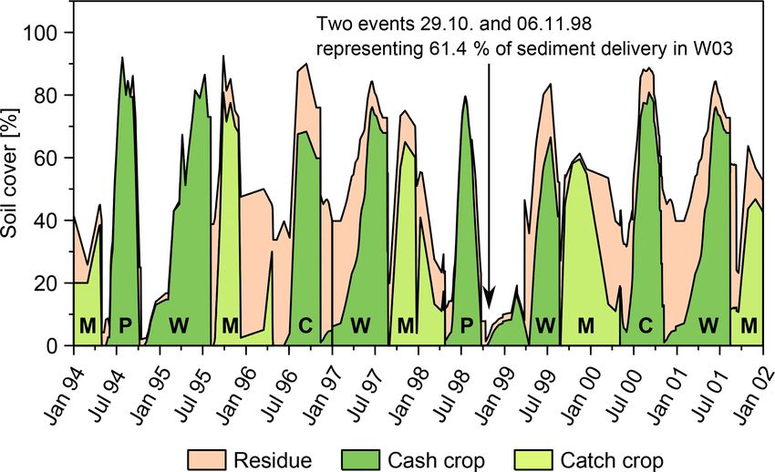
Figure 6. Averaged soil cover derived from measurements within
the field drained by watersheds W03 and W04; between 1994 and
1996 the cover was measured; from 1997 to 2001 the soil cover was
derived from the average cover measurements (1994–1996), taking
into account the crop and the year-specific times of field operations
within the test field occurring from 1997 to 2001 (W: wheat, C:
maize, P: potato, M: mustard used as catch crop) (modified after
Fiener et al., 2008). The arrow indicates the timing of the combined
largest two soil delivery events in this watershed.                     Figure 7. K factor map of the research farm; K factor was deter-
                                                                        mined according to Wischmeier et al. (1971) at the sampling lo-
                                                                        cations from measured soil properties and then geostatistically in-
                                                                        terpolated for 12.5 m × 12.5 m blocks. The krige standard deviation
                                                                        was about 0.02 t h ha−1 N−1 . The small panel displays the experi-
was only 9.7 N h−1 , which is one tenth of the mean annual              mental semivariogram calculated from 544 sampling locations and
erosivity. This event did not result in substantial erosion in          a spherical semivariogram model.
the other watersheds. This extreme event was able to take
place because the field in W03 was at seedbed conditions
for winter wheat after potato had been harvested four weeks             robust prediction of extremes that are mostly of highest rele-
earlier. Therefore, the field had no soil cover at all (see ar-         vance.
row Fig. 6) and the soil structure was substantially damaged               Equally important as the temporal dynamics of farming
by potato harvest. Furthermore, a smaller event one week be-            activities that affect soil cover and other properties are de-
fore the extreme event (#228) had already produced a rill net-          tailed data regarding spatial and spatio-temporal variabil-
work, which increased the sediment connectivity during the              ity of natural drivers. Within short distances almost the en-
largest event. Both events together comprised 61.4 % of all             tire range of soil erodibilities can be found in the study
sediment delivery measured during the 8 years in watershed              area (Fig. 7). The K factor at the grid nodes ranged from
W03. Watershed W03 was under integrated arable manage-                  0.03 to 0.65 t h ha−1 N−1 , while it ranged from 0.09 to
ment, which in general, produced the largest events, while              0.47 t h ha−1 N−1 for the 12.5 m × 12.5 m blocks (Fig. 7) de-
arable land and grassland under organic management showed               rived from the grid nodes. Only 3.5 % of all 20 000 soils
substantially lower event-based sediment delivery (Table 4).            covering Germany, that were analysed by Auerswald et
Under organic management, all extremes (except for W15)                 al. (2014), had a K factor outside this range that can al-
occurred in late winter to early spring and were associated             ready be found within the 150 ha of the research farm. This
with snowmelt and/or prolonged rainfall with minor event                fact points to a large and short-distance variability in hilly
rainfall erosivity (Table 4). In contrast, extremes (except for         terrain, were gravely, sandy and clayey Tertiary material is
W06 which produced anyway very small sediment delivery                  partly covered by Pleistocene loess. The pronounced short-
rates (Tables 3, 4)) under integrated farming were associated           range variability was even more evident from the semivari-
with large erosivities and times of low soil cover similar to           ogram (Fig. 7, small panel), which indicated a strong pattern
event #229 in W03.                                                      with a range of only 98 m. In other words, the entire K factor
   Without such detailed watershed data, it is hardly possi-            variation can be found within a distance of only 100 m.
ble to understand the processes driving such a series of large             The differences in soils between most watersheds under
events. A lack of such detailed data becomes especially crit-           integrated vs. organic farming, as evident also from the K
ical if runoff and sediment delivery data are used for model            factor (compare Figs. 2 and 7), was potentially one of the
development and testing. Large events play an essential role            reasons why watersheds under integrated farming produced
in model development, calibration, and testing to ensure a              larger events mostly during summer, while watersheds under

www.adv-geosci.net/48/31/2019/                                                                          Adv. Geosci., 48, 31–48, 2019
42                                                                  P. Fiener et al.: Filling the gap between plot and landscape scale

Table 3. Characteristics of measured surface runoff and sediment delivery events (W01 . . . W07, W10, W12 . . . W16: 1994–2001; W11:
1998–2001) in the different watersheds; C.V. is coefficient of variation. “Sum” is the total of eight years while all other columns are event
based. In total 287 events were recorded that produced runoff in at least one of the watersheds.

 Water-shed   Events                       Surface runoff [mm]                                          Sediment delivery [kg ha−1 ]
 No.              n    8-year   Event     SD    Event   C.V.     Skewness   Kurtosis   8-year   Event     SD      Event   C.V.   Skewness     Kurtosis
                         Sum    mean             max.                                    Sum    mean               max.
 W01            275      347     1.62    4.20    47.0   261           6.9        66     1293      6.0    16.1      141     268          5.4        34
 W02            270      500     2.49    6.06    46.8   244           4.3        22     2945     14.7    73.6     1002     503         12.3       164
 W03            287      324     1.47    4.59    42.0   314           5.4        36     3553     16.1   121.4     1715     756         12.8       177
 W04            173      319     1.98   14.61   146.9   739           9.0        82     3710     23.0   231.3     2891    1005         12.1       150
 W05            233      249     1.17    4.52    37.7   388           6.4        45     1521      7.1    48.7      608     682         10.7       123
 W06            229       71     0.41    1.31    11.1   322           5.7        37      146      0.8     2.9       30     350          7.3        65
 W07            123       39     0.47    2.03    17.1   432           7.1        56       70      0.8     2.7       15     322          3.9        16
 W10             69       19     0.50    2.21    13.1   442           5.4        30       31      0.8     3.5       20     432          5.1        27
 W11            112      174     1.56    5.07    31.9   326           4.5        22      311      2.8     9.5       67     339          4.9        27
 W12             71       42     0.60    2.40    17.9   404           5.9        40       92      1.3     5.0       36     383          5.6        36
 W13            107      137     0.12    0.61     6.1   516           9.1        89      437      4.1    29.0      295     712          9.7        98
 W14            152      182     1.67    4.12    32.6   247           4.9        31      329      3.0     7.9       55     263          4.5        23
 W15            246      127     0.62    1.81    14.6   290           4.8        26      333      1.6     6.7       80     406          9.1       100
 W16            216      273     1.71    3.35    28.2   197           4.3        26     1078      6.7    17.6      128     262          5.2        30

organic farming produced generally smaller events occurring
mostly in winter. This association between soils and farm-
ing practices was intentionally created in the design of the
study as it reflects agricultural practice. Thus, organic farm-
ing can be predominantly found on less fertile soils compared
to conventional farming (Auerswald et al., 2003). Neverthe-
less, due to a large number of adjoining watersheds, both
land-use systems can be compared under similar soil con-
ditions.
   More generally, the dataset indicated that a comparison
of watersheds with different land use or management can
only be reasonably done if the variability in soil properties
is taken into account. This is even more important for vari-
ables with pronounced spatio-temporal dynamics like field-
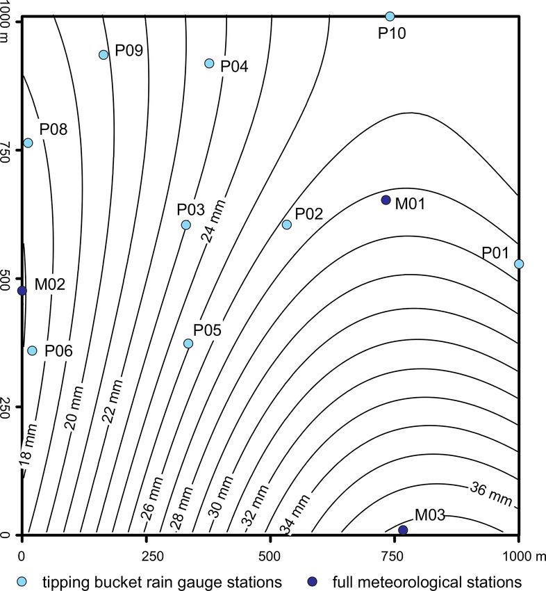
specific soil cover (Fig. 6) or spatial rainfall gradients of large
events (Fig. 8). The latter were studied at the test site for four
years using 12 rain gauges. These data indicated that 50 %
of all erosive events had substantial spatial rainfall gradients.
Variation in rain erosivity was up to 255 % and thus much
more pronounced than the variation in total rain depth (for
details see Fiener and Auerswald, 2009). Even for the rain-
fall event with the largest erosivity (approximately half of
the long-term mean annual erosivity) in the data set, erosiv-                Figure 8. Geostatistically interpolated rain depth (mm) of an ero-
ity was zero within a distance of about 500 m (Fischer et al.,               sive event with a substantial rainfall gradient (event 116, 26 Au-
2018). By analysing a much larger data set of about 40 000                   gust 1996); average rain depth calculated from the geostatistical in-
erosive events in Germany, Fischer et al. (2018) showed that                 terpolation in 10 m×10 m blocks was 23.6 mm and average gradient
this extreme behaviour of including zero within such a short                 in rain depth was 15.7 mm km−1 . Figure adapted from Fiener and
distance was true for about half of all events but that strong               Auerswald (2009).
gradients existed also for most of the other events. This em-
phasized that also for small watersheds, spatial variability in
rainfall has to be taken into account.                                       4   Conclusions

                                                                             Watershed studies are indispensable to understand soil ero-
                                                                             sion as they integrate (i) real agricultural practices, (ii) nat-
                                                                             ural heterogeneity along the flow path, and (iii) realistic

Adv. Geosci., 48, 31–48, 2019                                                                                   www.adv-geosci.net/48/31/2019/
You can also read