MC-LSTM: MASS-CONSERVING LSTM - OpenReview
←
→
Page content transcription
If your browser does not render page correctly, please read the page content below
Under review as a conference paper at ICLR 2021

MC-LSTM: M ASS -C ONSERVING LSTM
 Anonymous authors
 Paper under double-blind review

                                              A BSTRACT

         The success of Convolutional Neural Networks (CNNs) in computer vision is
         mainly driven by their strong inductive bias, which is strong enough to allow
         CNNs to solve vision-related tasks with random weights, meaning without learning.
         Similarly, Long Short-Term Memory (LSTM) has a strong inductive bias towards
         storing information over time. However, many real-world systems are governed
         by conservation laws, which lead to the redistribution of particular quantities —
         e.g. in physical and economical systems. Our novel Mass-Conserving LSTM
         (MC-LSTM) adheres to these conservation laws by extending the inductive bias of
         LSTM to model the redistribution of those stored quantities. MC-LSTMs set a new
         state-of-the-art for neural arithmetic units at learning arithmetic operations, such as
         addition tasks, which have a strong conservation law, as the sum is constant over
         time. Further, MC-LSTM is applied to traffic forecasting, modeling a pendulum,
         and a large benchmark dataset in hydrology, where it sets a new state-of-the-art for
         predicting peak flows. In the hydrology example, we show that MC-LSTM states
         correlate with real world processes and are therefore interpretable.

1   I NTRODUCTION

Inductive biases enabled the success of CNNs and LSTMs. One of the greatest success stories
of deep learning is Convolutional Neural Networks (CNNs) (Fukushima, 1980; LeCun & Bengio,
1998; Schmidhuber, 2015; LeCun et al., 2015) whose proficiency can be attributed to their strong
inductive bias towards visual tasks (Cohen & Shashua, 2017; Gaier & Ha, 2019). The effect of this
inductive bias has been demonstrated by CNNs that solve vision-related tasks with random weights,
meaning without learning (He et al., 2016; Gaier & Ha, 2019; Ulyanov et al., 2020). Another success
story is Long Short-Term Memory (LSTM) (Hochreiter, 1991; Hochreiter & Schmidhuber, 1997),
which has a strong inductive bias toward storing information through its memory cells. This inductive
bias allows LSTM to excel at speech, text, and language tasks (Sutskever et al., 2014; Bohnet et al.,
2018; Kochkina et al., 2017; Liu & Guo, 2019), as well as timeseries prediction. Even with random
weights and only a learned linear output layer LSTM is better at predicting timeseries than reservoir
methods (Schmidhuber et al., 2007). In a seminal paper on biases in machine learning, Mitchell
(1980) stated that “biases and initial knowledge are at the heart of the ability to generalize beyond
observed data”. Therefore, choosing an appropriate architecture and inductive bias for deep neural
networks is key to generalization.

Mechanisms beyond storing are required for real-world applications. While LSTM can store
information over time, real-world applications require mechanisms that go beyond storing. Many
real-world systems are governed by conservation laws related to mass, energy, momentum, charge, or
particle counts, which are often expressed through continuity equations. In physical systems, different
types of energies, mass or particles have to be conserved (Evans & Hanney, 2005; Rabitz et al., 1999;
van der Schaft et al., 1996), in hydrology it is the amount of water (Freeze & Harlan, 1969; Beven,
2011), in traffic and transportation the number of vehicles (Vanajakshi & Rilett, 2004; Xiao & Duan,
2020; Zhao et al., 2017), and in logistics the amount of goods, money or products. A real-world
task could be to predict outgoing goods from a warehouse based on a general state of the warehouse,
i.e., how many goods are in storage, and incoming supplies. If the predictions are not precise, then
they do not lead to an optimal control of the production process. For modeling such systems, certain
inputs must be conserved but also redistributed across storage locations within the system. We will
    All code to reproduce the results will be made available on GitHub.

                                                     1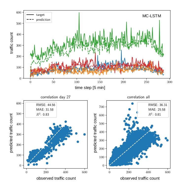
Under review as a conference paper at ICLR 2021

refer to conserved inputs as mass, but note that this can be any type of conserved quantity. We argue
that for modeling such systems, specialized mechanisms should be used to represent locations &
whereabouts, objects, or storage & placing locations and thus enable conservation.

Conservation laws should pervade machine learning models in the physical world. Since a
large part of machine learning models are developed to be deployed in the real world, in which
conservation laws are omnipresent rather than the exception, these models should adhere to them
automatically and benefit from them. However, standard deep learning approaches struggle at
conserving quantities across layers or timesteps (Beucler et al., 2019b; Greydanus et al., 2019; Song
& Hopke, 1996; Yitian & Gu, 2003), and often solve a task by exploiting spurious correlations
(Szegedy et al., 2014; Lapuschkin et al., 2019). Thus, an inductive bias of deep learning approaches
via mass conservation over time in an open system, where mass can be added and removed, could
lead to a higher generalization performance than standard deep learning for the above-mentioned
tasks.

A mass-conserving LSTM. In this work, we introduce Mass-Conserving LSTM (MC-LSTM),
a variant of LSTM that enforces mass conservation by design. MC-LSTM is a recurrent neural
network with an architecture inspired by the gating mechanism in LSTMs. MC-LSTM has a strong
inductive bias to guarantee the conservation of mass. This conservation is implemented by means
of left-stochastic matrices, which ensure the sum of the memory cells in the network represents the
current mass in the system. These left-stochastic matrices also enforce the mass to be conserved
through time. The MC-LSTM gates operate as control units on mass flux. Inputs are divided into
a subset of mass inputs, which are propagated through time and are conserved, and a subset of
auxiliary inputs, which serve as inputs to the gates for controlling mass fluxes. We demonstrate that
MC-LSTMs excel at tasks where conservation of mass is required and that it is highly apt at solving
real-world problems in the physical domain.

Contributions. We propose a novel neural network architecture based on LSTM that conserves
quantities, such as mass, energy, or count, of a specified set of inputs. We show properties of this
novel architecture, called MC-LSTM, and demonstrate that these properties render it a powerful
neural arithmetic unit. Further, we show its applicability in real-world areas of traffic forecasting and
modeling the pendulum. In hydrology, large-scale benchmark experiments reveal that MC-LSTM
has powerful predictive quality and can supply interpretable representations.

2   M ASS -C ONSERVING LSTM
The original LSTM introduced memory cells to Recurrent Neural Networks (RNNs), which alleviate
the vanishing gradient problem (Hochreiter, 1991). This is achieved by means of a fixed recurrent
self-connection of the memory cells. If we denote the values in the memory cells at time t by ct , this
recurrence can be formulated as
                                      ct = ct−1 + f (xt , ht−1 ),                                    (1)
where x and h are, respectively, the forward inputs and recurrent inputs, and f is some function
that computes the increment for the memory cells. Here, we used the original formulation of LSTM
without forget gate (Hochreiter & Schmidhuber, 1997), but in all experiments we also consider LSTM
with forget gate (Gers et al., 2000).
MC-LSTMs modify this recurrence to guarantee the conservation of the mass input.The key idea is
to use the memory cells from LSTMs as mass accumulators, or mass storage. The conservation law
is implemented by three architectural changes. First, the increment, computed by f in Eq. (1), has to
distribute mass from inputs into accumulators. Second, the mass that leaves MC-LSTM must also
disappear from the accumulators. Third, mass has to be redistributed between mass accumulators.
These changes mean that all gates explicitly represent mass fluxes.
Since, in general, not all inputs must be conserved, we distinguish between mass inputs, x, and
auxiliary inputs, a. The former represents the quantity to be conserved and will fill the mass
accumulators in MC-LSTM. The auxiliary inputs are used to control the gates. To keep the notation
uncluttered, and without loss of generality, we use a single mass input at each timestep, xt , to
introduce the architecture.

                                                   2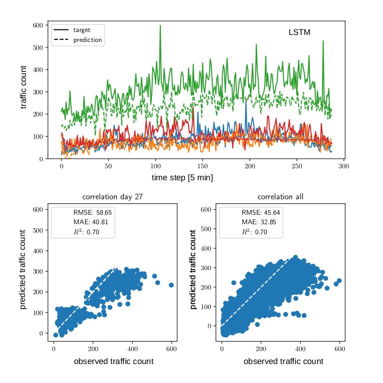
Under review as a conference paper at ICLR 2021

The forward pass of MC-LSTM at timestep t
can be specified as follows:

          mttot = Rt · ct−1 + it · xt         (2)
              t           t
             c = (1 − o )         mttot       (3)
              t     t
             h =o       mttot .               (4)

where it and ot are the input- and output gates,
respectively, and R is a positive left-stochastic
matrix, i.e., 1T · R = 1, for redistributing mass Figure 1: Schematic representation of the main
in the accumulators. The total mass mtot is operations in the MC-LSTM architecture (adapted
the redistributed mass, Rt · ct−1 , plus the mass from: Olah, 2015).
influx, or new mass, it · xt . The current mass in
the system is stored in ct .
Note the differences between Eq. (1) and Eq. (3). First, the increment of the memory cells no
longer depends on ht . Instead, mass inputs are distributed by means of the normalized i (see Eq. 5).
Furthermore, Rt replaces the implicit identity matrix of LSTM to redistribute mass among memory
cells. Finally, Eq. (3) introduces 1 − ot as a forget gate on the total mass, mtot . Together with
Eq. (4), this assures that no outgoing mass is stored in the accumulators. This formulation has some
similarity to Gated Recurrent Units (GRU) (Cho et al., 2014), however the gates are not used for
mixing the old and new cell state, but for splitting off the output.

Basic gating and redistribution. The MC-LSTM gates at timestep t are computed as follows:
                                                               ct−1
                              it = softmax(W i · at + U i ·            + bi )                     (5)
                                                              kct−1 k1
                                                         ct−1
                              ot = σ(W o · at + U o ·            + bo )                           (6)
                                                        kct−1 k1
                          Rt = softmax(B r ),                                                     (7)
where the softmax operator is applied column-wise, σ is the logistic sigmoid function, and W i , bi ,
W o , bo , and B r are learnable model parameters. Note that for the input gate and redistribution
matrix, the requirement is that they are column normalized. This can also be achieved by other means
than using the softmax function. For example, an alternative way to ensure a column-normalized
                                                       σ(rkj )
matrix Rt is to use a normalized logistic, σ̃(rkj ) = P σ(r kn )
                                                                 . Also note that MC-LSTMs compute
                                                        n
the gates from the memory cells, directly. This is in contrast with the original LSTM, which uses
the activations from the previous time step. The accumulated values from the memory cells, ct , are
normalized to counter saturation of the sigmoids and to supply probability vectors that represent the
current distribution of the mass across cell states We use this variation e.g. in our experiments with
neural arithmetics (see Sec. 5.1).

Time-dependent redistribution. It can also be useful to predict a redistribution matrix for each
sample and timestep, similar to how the gates are computed:
                                                         ct−1

                        Rt = softmax Wr · at + Ur · t−1 + B r ,                               (8)
                                                        kc k1
where the parameters Wr and Ur are weight tensors and their multiplications result in K ×K matrices.
Again, the softmax function is applied column-wise. This version collapses to a time-independent
redistribution matrix if Wr and Ur are equal to 0. Thus, there exists the option to initialize Wr and
Ur with weights that are small in absolute value compared to the weights of B r , to favour learning
time-independent redistribution matrices. We use this variant in the hydrology experiments (see
Sec. 5.4).
Redistribution via a hypernetwork. Even more general, a hypernetwork (Schmidhuber, 1992; Ha
et al., 2017) that we denote with g can be used to procure R. The hypernetwork has to produce

                                                    3
Under review as a conference paper at ICLR 2021
a column-normalized, square matrix Rt = g(a0 , . . . , at , c0 , . . . , ct−1 ). Notably, a hypernetwork
can be used to design an autoregressive version of MC-LSTMs, if the network additionally predicts
auxiliary inputs for the next time step. We use this variant in the pendulum experiments (see Sec. 5.3).
3 P ROPERTIES
Conservation. MC-LSTM guarantees that mass is conserved over time. This is a direct conse-
quence of connecting memory cells with stochastic matrices. The mass conservation ensures that no
mass can be removed or added implicitly, which makes it easier to learn functions that generalize
well. The exact meaning of this mass conservation is formalized in Theorem 1.
PK
Theorem 1 (Conservation property). Let mτc = k=1 cτk be the mass contained in the system and
PK
mτh = k=1 hτk be the mass efflux, or, respectively, the accumulated mass in the MC-LSTM storage
and the outputs at time τ . At any timestep τ , we have:
τ
X τ
X
mτc = m0c + xt − mth . (9)
t=1 t=1
That is, the change of mass in the memory cells is the difference between the input and output mass,
accumulated over time.
The proof is by induction over τ (see Appendix C). Note that it is still possible for input mass to
be stored indefinitely in a memory cell so that it does not appear at the output. This can be a useful
feature if not all of the input mass is needed at the output. In this case, the network can learn that one
cell should operate as a collector for excess mass in the system.
τ
Boundedness Pof
τ
cell states. In each timestepPτ τ , the memory cells, ck , are bounded by the sum of
mass inputs t=1 xtP + m0c , that is |cτk | ≤ t=1 xt + m0c . Furthermore, if the series of mass inputs
τ
converges, limτ →∞ t=1 xτ = m∞ x , then also the sum of cell states converges (see Appendix,
Corollary 1).
Initialization and gradient flow. MC-LSTM with Rt = I has a similar gradient flow to LSTM
with forget gate (Gers et al., 2000). Thus, the main difference in the gradient flow is determined
by the redistribution matrix R. The forward pass of MC-LSTM without gates ct = Rt ct−1 leads
t
to the following backward expression ∂c∂ct−1 = Rt . Hence, MC-LSTM should be initialized with a
redistribution matrix close to the identity matrix to ensure a stable gradient flow as in LSTMs. For
random redistribution matrices, the circular law theorem for random Markov matrices (Bordenave
et al., 2012) can be used to analyze the gradient flow in more detail, see Appendix, Section D.
Computational complexity. Whereas the gates in a traditional LSTM are vectors, the input gate
and redistribution matrix of an MC-LSTM are matrices in the most general case. This means that
MC-LSTM is, in general, computationally more demanding than LSTM. Concretely, the forward pass
for a single timestep in MC-LSTM requires O(K 3 + K 2 (M + L) + KM L) Multiply-Accumulate
operations (MACs), whereas LSTM takes O(K 2 + K(M + L)) MACs per timestep. Here, M , L
and K are the number of mass inputs, auxiliary inputs and outputs, respectively. When using a time-
independent redistribution matrix cf. Eq. (7), the complexity reduces to O(K 2 M + KM L) MACs.
Potential interpretability through inductive bias and accessible mass in cell states. The repre-
sentations within the model can be interpreted directly as accumulated mass. If one mass or energy
quantity is known, the MC-LSTM architecture would allow to force a particular cell state to represent
this quantity, which could facilitate learning and interpretability. An illustrative example is the case
of rainfall runoff modelling, where observations, say of the soil moisture or groundwater-state, could
be used to guide the learning of an explicit memory cell of MC-LSTM.
4Under review as a conference paper at ICLR 2021
4 S PECIAL CASES AND RELATED WORK
Relation to Markov chains. In a special case MC-LSTM collapses to a finite Markov chain, when
c0 is a probability vector, the mass input is zero xt = 0 for all t, there is no input and output gate, and
the redistribution matrix is constant over time Rt = R. For finite Markov chains, the dynamics are
known to converge, if R is irreducible (see e.g. Hairer (2018, Theorem 3.13.)). Awiszus & Rosenhahn
(2018) aim to model a Markov Chain by having a feed-forward network predict the state distribution
given the current state distribution. In order to insert randomness to the network, a random seed is
appended to the input, which allows to simulate Markov processes. Although MC-LSTMs are closely
related to Markov chains, they do not explicitly learn the transition matrix, as is the case for Markov
chain neural networks. MC-LSTMs would have to learn the transition matrix implicitly.
Relation to normalizing flows and volume-conserving neural networks. In contrast to normal-
izing flows (Rezende & Mohamed, 2015; Papamakarios et al., 2019), which transform inputs in each
layer and trace their density through layers or timesteps, MC-LSTMs transform distributions and do
not aim to trace individual inputs through timesteps. Normalizing flows thereby conserve information
about the input in the first layer and can use the inverted mapping to trace an input back to the
initial space. MC-LSTMs are concerned with modeling the changes of the initial distribution over
time and can guarantee that a multinomial distribution is mapped to a multinomial distribution. For
MC-LSTMs without gates, the sequence of cell states c0 , . . . , cT constitutes a normalizing flow if
an initial distribution p0 (c0 ) is available. In more detail, MC-LSTM can be considered a linear flow
with the mapping ct+1 = Rt ct and p(ct+1 ) = p(ct )| det Rt |−1 in this case. The gate providing the
redistribution matrix (see Eq. 8) is the conditioner in a normalizing flow model. From the perspective
of normalizing flows, MC-LSTM can be considered as a flow trained in a supervised fashion. Deco
& Brauer (1995) proposed volume-conserving neural networks, which conserve the volume spanned
by input vectors and thus the information of the starting point of an input is kept. In other words, they
are constructed so that the Jacobians of the mapping from one layer to the next have a determinant
of 1. In contrast, the MC-LSTMs determinant of the Jacobians (of the mapping) is smaller than 1
(except for degenerate cases), which means that volume of the inputs is not conserved.
Relation to Layer-wise Relevance Propagation. Layer-wise Relevance Propagation (LRP) (Bach
et al., 2015) is similar to our approach with respect to the idea that the sum of a quantity, the
relevance Ql is conserved over layers l. LRP aims to maintain the sum of the relevance values
PI l−1 PI
k=1 Qi = k=1 Ql−1 i backward through a classifier in order to a obtain relevance values for
each input feature.
Relation to other networks that conserve particular properties. While a standard feed-forward
neural network does not give guarantees aside from the conservation of the proximity of datapoints
through the continuity property. The conservation of the first moments of the data distribution in
the form of normalization techniques (Ioffe & Szegedy, 2015) has had tremendous success. Here,
batch normalization (Ioffe & Szegedy, 2015) could exactly conserve mean and variance across layers,
whereas self-normalization (Klambauer et al., 2017) conserves those approximately. The conservation
of the spectral norm of each layer in the forward pass has enabled the stable training of generative
adversarial networks (Miyato et al., 2018). The conservation of the spectral norm of the errors
through the backward pass of an RNN has enabled the avoidance of the vanishing gradient problem
(Hochreiter, 1991; Hochreiter & Schmidhuber, 1997). In this work, we explore an architecture that
exactly conserves the mass of a subset of the input, where mass is defined as a physical quantity such
as mass or energy.
Relation to neural networks for physical systems. Neural networks have been shown to discover
physical concepts such as the conservation of energies (Iten et al., 2020), and neural networks could
allow to learn natural laws from observations (Schmidt & Lipson, 2009; Cranmer et al., 2020b).
MC-LSTM can be seen as a neural network architecture with physical constraints (Karpatne et al.,
2017; Beucler et al., 2019c). It is however also possible to impose conservation laws by using other
means, e.g. initialization, constrained optimization or soft constraints (as, for example, proposed by
Karpatne et al., 2017; Beucler et al., 2019c;a; Jia et al., 2019). Hamiltonian neural networks (Grey-
danus et al., 2019) and Symplectic Recurrent Neural Networks make energy conserving predictions
by using the Hamiltonian (Chen et al., 2019), a function that maps the inputs to the quantity that
5Under review as a conference paper at ICLR 2021
Table 1: Performance of different models on the LSTM addition task in terms of the MSE. MC-LSTM
significantly (all p-values below .05) outperforms its competitors, LSTM (with high initial forget
gate bias), NALU and NAU. Error bars represent 95%-confidence intervals across 100 runs.
referencea seq lengthb input rangec countd comboe NaNf
MC-LSTM 0.004 ± 0.003 0.009 ± 0.004 0.8 ± 0.5 0.6 ± 0.4 4.0 ± 2.5 0
LSTM 0.008 ± 0.003 0.727 ± 0.169 21.4 ± 0.6 9.5 ± 0.6 54.6 ± 1.0 0
NALU 0.060 ± 0.008 0.059 ± 0.009 25.3 ± 0.2 7.4 ± 0.1 63.7 ± 0.6 93
NAU 0.248 ± 0.019 0.252 ± 0.020 28.3 ± 0.5 9.1 ± 0.2 68.5 ± 0.8 24
a
training regime: summing 2 out of 100 numbers between 0 and 0.5.
b
longer sequence lengths: summing 2 out of 1 000 numbers between 0 and 0.5.
c
more mass in the input: summing 2 out of 100 numbers between 0 and 5.0.
d
higher number of summands: summing 20 out of 100 numbers between 0 and 0.5.
e
combination of previous scenarios: summing 10 out of 500 numbers between 0 and 2.5.
f
Number of runs that did not converge.
needs to be conserved. By using the symplectic gradients, it is possible to move around in the input
space, without changing the output of the Hamiltonian. Lagrangian Neural Networks (Cranmer et al.,
2020a), extend the Hamiltonian concept by making it possible to use arbitrary coordinates as inputs.
All of these approaches, while very promising, assume closed physical systems and are thus to
restrictive for the application we have in mind. Raissi et al. (2019) propose to enforce physical
constraints on simple feed-forward networks by computing the partial derivatives with respect to
the inputs and computing the partial differential equations explicitly with the resulting terms. This
approach, while promising, does require an exact knowledge of the governing equations. By contrast,
our approach is able to learn its own representation of the underlying process, while obeying the
pre-specified conservation properties.
5 E XPERIMENTS
In the following, we discuss the experiments we conducted to demonstrate the broad applicability and
high predictive performance of MC-LSTM in settings where mass conservation is required. For more
details on the datasets and hyperparameter selection for each experiment, we refer to Appendix B.
5.1 A RITHMETIC TASKS
Addition problem. We first considered a problem for which exact mass conservation is required.
One example for such a problem has been described in the original LSTM paper (Hochreiter &
Schmidhuber, 1997), showing that LSTM is capable of summing two arbitrarily marked elements in a
sequence of random numbers. We show that MC-LSTM is able to solve this task, but also generalizes
better to longer sequences, input values in a different range and more summands. Table 1 summarizes
the results of this method comparison and shows that MC-LSTM significantly outperformed the other
models on all tests (p-value ≤ 0.03, Wilcoxon test). In Appendix B.1.5, we provide a qualitative
analysis of the learned model behavior for this task.
Recurrent arithmetic. Following Madsen & Johansen (2020), the inputs for this task are sequences
of vectors, uniformly drawn from [1, 2]10 . For each vector in the sequence, the sum over two random
subsets is calculated. Those values are then summed over time, leading to two values. The target
output is obtained by applying the arithmetic operation to these two values. The auxiliary input for
MC-LSTM is a sequence of ones, where the last element is −1 to signal the end of the sequence.
We evaluated MC-LSTM against NAUs and Neural Accumulators (NACs) directly in the framework
of Madsen & Johansen (2020). NACs and NAUs use the architecture as presented in (Madsen &
Johansen, 2020). That is, a single hidden layer with two neurons, where the first layer is recurrent.
The MC-LSTM model has two layers, of which the second one is a fully connected linear layer. For
subtraction an extra cell was necessary to properly discard redundant input mass.
6Under review as a conference paper at ICLR 2021
Table 2: Recurrent arithmetic task results. MC-LSTMs for addition and subtraction/multiplication
have two and three neurons, respectively. Error bars represent 95%-confidence intervals.
addition subtraction multiplication
a b a b
success rate updates success rate updates success ratea updatesb
MC-LSTM 96% +2%
−6% 4.6 · 105 81% +6%
−9% 1.2 · 105 67% +8%
−10% 1.8 · 105
NAU / NMU 88% +5%
−8% 8.1 · 104 60% +9%
−10% 6.1 · 104 34% +10%
−9% 8.5 · 104
NAC 56% +9%
−10% 3.2 · 105 86% +5%
−8% 4.5 · 104 0% +4%
−0% –
NALU 10% +7%
−4% 1.0 · 106 0% +4%
−0% – 1% +4%
−1% 4.3 · 105
a
Percentage of runs that generalized to longer sequences.
b
Median number of updates necessary to solve the task.
Success rate
For testing, we took the model with the lowest val- 1.00
idation error, c.f. early stopping. The performance ●
●
●
● ● ● ● ● ● ●
0.75 ●
was measured by the percentage of runs that suc- ●
cessfully generalized to longer sequences. General- 0.50
ization is considered successful if the error is lower
than the numerical imprecision of the exact opera- 0.25 MC-LSTM NAU ● ●
tion (Madsen & Johansen, 2020). The summary in
Tab. 2 shows that MC-LSTM was able to significantly 0.00
1 10 200 400 600 800 1000
outperform the competing models (p-value 0.03 for Sequence length
addition and 3e−6 for multiplication, proportion test).
In Appendix B.1.5, we provide a qualitative analysis Figure 2: MNIST arithmetic task results for
of the learned model behavior for this task. MC-LSTM and NAU. The task is to correctly
predict the sum of a sequence of presented
Static arithmetic. To enable a direct comparison MNIST digits. The success rates are depicted
with the results reported in Madsen & Johansen on the y-axis in dependency of the length of
(2020), we also compared MC-LSTM on the static the sequence (x-axis) of MNIST digits. Error
arithmetic task, see Appendix B.1.3. bars represent 95%-confidence intervals.
MNIST arithmetic. We tested that feature extractors can be learned from MNIST images (LeCun
et al., 1998) to perform arithmetic on the images (Madsen & Johansen, 2020). The input is a sequence
of MNIST images and the target output is the corresponding sum of the labels. Auxiliary inputs are
all 1, except the last entry, which is −1, to indicate the end of the sequence. The models are the
same as in the recurrent arithmetic task with CNN to convert the images to (mass) inputs for these
networks. The network is learned end-to-end. L2 -regularization is added to the output of CNN to
prevent its outputs from growing arbitrarily large. The results for this experiment are depicted in
Fig. 2. MC-LSTM significantly outperforms the state-of-the-art, NAU (p-value 0.002, Binomial test).
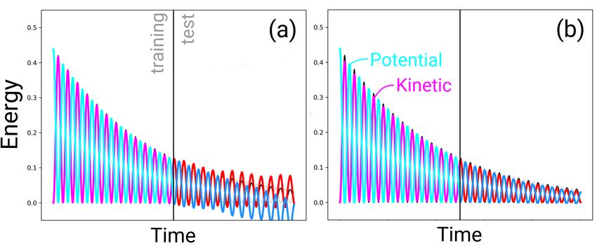
5.2 I NBOUND - OUTBOUND TRAFFIC FORECASTING
We examined the usage of MC-LSTMs for traffic fore-
casting in situations in which inbound and outbound
traffic counts of a city are available (see Fig. 3). For this
type of data, a conservation-of-vehicles principle (Nam
& Drew, 1996) must hold, since vehicles can only leave
the city if they have entered it before or had been there
in the first place. Based on data for the traffic4cast 2020
challenge (Kreil et al., 2020), we constructed a dataset
to model inbound and outbound traffic in three differ-
ent cities: Berlin, Istanbul and Moscow. We compared Figure 3: Schematic depiction of inbound-
MC-LSTM against LSTM, which is the state-of-the-art outbound traffic situations that require the
method for several types of traffic forecasting situations conservation-of-vehicles principle. All ve-
(Zhao et al., 2017; Tedjopurnomo et al., 2020), and hicles on outbound roads (yellow arrows)
found that MC-LSTM significantly outperforms LSTM must have entered the city center before
in this traffic forecasting setting (all p-values ≤ 0.01, (green arrows) or have been present in the
Wilcoxon test). For details, see Appendix B.2. first timestep.
7Under review as a conference paper at ICLR 2021
5.3 P ENDULUM WITH FRICTION
In the area of physics, we examined the usability of MC-LSTM for the problem of modeling a swing-
ing pendulum with friction. Here, the total energy is the conserved property. During the movement
of the pendulum, kinetic energy is converted into potential energy and vice-versa. This conversion
between both energies has to be learned by the off-diagonal values of the redistribution matrix. A
qualitative analysis of a trained MC-LSTM for this problem can be found in Appendix B.3.1.
Accounting for friction, energy dissipates and
the swinging slows over time until towards a
fixed point. This type of behavior presents a
difficulty for machine learning and is impossi-
ble for methods that assume the pendulum to
be a closed system, such as Hamiltonian net-
works (Greydanus et al., 2019). We generated
120 datasets of timeseries data of a pendulum
where we used multiple different settings for
initial angle, length of the pendulum, and the
amount of friction. We then selected LSTM Figure 4: Example for the pendulum-modelling
and MC-LSTM models and compared them exercise. (a) LSTM trained for predicting energies
with respect to predictive MSE. For an exam- of the pendulum with friction in auto-regressive
ple, see Fig. 4. Overall, MC-LSTM has signif- fashion, (b) MC-LSTM trained in the same set-
icantly outperformed LSTM with a mean MSE ting. Each subplot shows the potential- and kinetic
of 0.01 (standard deviation 0.04) compared to energy and the respective predictions.
0.05 (standard deviation 0.15; with a p-value
6.9e−8, Wilcoxon test).
5.4 H YDROLOGY: RAINFALL RUNOFF MODELING
We tested MC-LSTM for large-sample hydrological modeling following Kratzert et al. (2019c). An
ensemble of 10 MC-LSTMs was trained on 10 years of data from 447 basins using the publicly-
available CAMELS dataset (Newman et al., 2015; Addor et al., 2017a). The mass input is precipitation
and auxiliary inputs are: daily min. and max. temperature, solar radiation, and vapor pressure, plus 27
basin characteristics related to geology, vegetation, and climate (described by Kratzert et al., 2019c).
All models besides MC-LSTM and LSTM were trained by different research groups with experience
using each model. More details are given in Appendix B.4.2.
As shown in Tab. 3 MC-LSTM performed better Table 3: Hydrology benchmark results. All val-
with respect to the Nash–Sutcliffe Efficiency (NSE; ues represent the median (25% and 75% per-
the R2 between simulated and observed runoff) than centile in sub- and superscript, respectively)
any other mass-conserving hydrology model, al- over the 447 basins. Only the two best per-
though slightly worse than LSTM. forming hydrological models are included. An
extended version can be found in Tab. B.7.
NSE is often not the most important metric in hydrol-
ogy, since water managers are typically concerned
primarily with extremes (e.g. floods). MC-LSTM Model MCa FHVb NSEc
performed significantly better (p = 0.025, Wilcoxon −7.0
MC-LSTM 3 -14.7−23.4 0.7440.814
0.641
test) than all models, including LSTM, with respect −8.6
to high volume flows (FHV), at or above the 98th per- LSTM 7 -15.7−23.8 0.7630.835
0.676
−9.5
centile flow in each basin. This makes MC-LSTM mHM 3 -18.6−27.7 0.6660.730
0.588
the current state-of-the-art model for flood predic- ... ... ... ...
−8.5
tion. MC-LSTM also performed significantly better HBVub 3 -18.5−27.8 0.6760.749
0.578
than LSTM on low volume flows (FLV) and over- a
: Mass conservation (MC).
all bias, however there are other hydrology models b
: Top 2% peak flow bias: (−∞, ∞), values closer
that are better for predicting low flows (which is to zero are desirable.
c
important, e.g. for managing droughts). : Nash-Sutcliffe Efficiency: (−∞, 1], values closer
to one are desirable.
Model states and environmental processes. It is an open challenge to bridge the gap between the
fact that LSTM approaches give generally better predictions than other models (especially for flood
prediction) and the fact that water managers need predictions that help them understand not only how
much water will be in a river at a given time, but also how water moves through a basin.
8Under review as a conference paper at ICLR 2021
Snow processes are difficult to observe and model. Kratzert et al. (2019a) showed that LSTM learns
to track snow in memory cells without requiring snow data for training. We found similar behavior in
MC-LSTMs, which has the advantage of doing this with memory cells that are true mass storages.
Figure 5 shows the snow as the sum over a subset of MC-LSTM memory states and snow water
equivalent (SWE) modeled by the well-established Snow-17 snow model (Anderson, 1973) (Pearson
correlation coefficient r ≥ 0.91). It is important to remember that MC-LSTMs did not have access
to any snow data during training. In the best case it is possible to take advantage of the inductive
bias to predict how much water will be stored as snow under different conditions by using simple
combinations or mixtures of the internal states. Future work will determine whether this is possible
with other difficult-to-observe states and fluxes.
400
Snow Water Equivalent (mm)
Sum of MC-LSTM 'snow' cells
SWE (mm)
200
0
1981 1982 1983 1984 1985 1986 1987 1988 1989 1990
Date
Figure 5: Snow-water-equivalent (SWE) from a single basin. The blue line is SWE modeled
by Newman et al. (2015). The orange line is the sum over 4 MC-LSTM memory cells (Pearson
correlation coefficient r ≥ 0.8).
6 C ONCLUSION .
We have demonstrated that with the concept of inductive biases an RNN can be designed that has
the property to conserve mass of particular inputs. This architecture is highly proficient as neural
arithmetic unit and is well-suited for predicting physical systems like hydrological processes, in
which water mass has to be conserved.
R EFERENCES
Nans Addor, Andrew J Newman, Naoki Mizukami, and Martyn P Clark. The camels data set:
catchment attributes and meteorology for large-sample studies. Hydrology and Earth System
Sciences (HESS), 21(10):5293–5313, 2017a.
Nans Addor, Andrew J. Newman, Naoki Mizukami, and Martyn P. Clark. Catchment attributes for
large-sample studies. Boulder, CO: UCAR/NCAR, 2017b.
Eric A Anderson. National weather service river forecast system: Snow accumulation and ablation
model. NOAA Tech. Memo. NWS HYDRO-17, 87 pp., 1973.
Maren Awiszus and Bodo Rosenhahn. Markov chain neural networks. In 2018 IEEE/CVF Conference
on Computer Vision and Pattern Recognition Workshops (CVPRW), pp. 2261–22617, 2018.
Sebastian Bach, Alexander Binder, Grégoire Montavon, Frederick Klauschen, Klaus-Robert Müller,
and Wojciech Samek. On pixel-wise explanations for non-linear classifier decisions by layer-wise
relevance propagation. PloS one, 10(7):1–46, 2015.
Samy Bengio, Oriol Vinyals, Navdeep Jaitly, and Noam Shazeer. Scheduled sampling for sequence
prediction with recurrent neural networks. In Advances in Neural Information Processing Systems
28, pp. 1171–1179. Curran Associates, Inc., 2015.
Tom Beucler, Michael Pritchard, Stephan Rasp, Pierre Gentine, Jordan Ott, and Pierre Baldi. Enforc-
ing analytic constraints in neural-networks emulating physical systems, 2019a.
Tom Beucler, Stephan Rasp, Michael Pritchard, and Pierre Gentine. Achieving conservation of energy
in neural network emulators for climate modeling. arXiv preprint arXiv:1906.06622, 2019b.
9Under review as a conference paper at ICLR 2021
Tom Beucler, Stephan Rasp, Michael Pritchard, and Pierre Gentine. Achieving conservation of energy
in neural network emulators for climate modeling. ICML Workshop “Climate Change: How Can
AI Help?”, 2019c.
Keith Beven. Deep learning, hydrological processes and the uniqueness of place. Hydrological
Processes, 34(16):3608–3613, 2020.
Keith J Beven. Rainfall-runoff modelling: the primer. John Wiley & Sons, 2011.
Bernd Bohnet, Ryan McDonald, Goncalo Simoes, Daniel Andor, Emily Pitler, and Joshua Maynez.
Morphosyntactic tagging with a meta-bilstm model over context sensitive token encodings. arXiv
preprint arXiv:1805.08237, 2018.
Charles Bordenave, Pietro Caputo, and Djalil Chafai. Circular law theorem for random markov
matrices. Probability Theory and Related Fields, 152(3-4):751–779, 2012.
Zhengdao Chen, Jianyu Zhang, Martin Arjovsky, and Léon Bottou. Symplectic recurrent neural
networks. arXiv preprint arXiv:1909.13334, 2019.
Kyunghyun Cho, Bart van Merriënboer, Caglar Gulcehre, Dzmitry Bahdanau, Fethi Bougares, Holger
Schwenk, and Yoshua Bengio. Learning phrase representations using rnn encoder-decoder for
statistical machine translation. In Proceedings of the Conference on Empirical Methods in Natural
Language Processing, pp. 1724–1734. Association for Computational Linguistics, 2014.
N. Cohen and A. Shashua. Inductive bias of deep convolutional networks through pooling geometry.
In International Conference on Learning Representations, 2017.
Miles Cranmer, Sam Greydanus, Stephan Hoyer, Peter Battaglia, David Spergel, and Shirley Ho.
Lagrangian neural networks. arXiv preprint arXiv:2003.04630, 2020a.
Miles Cranmer, Alvaro Sanchez Gonzalez, Peter Battaglia, Rui Xu, Kyle Cranmer, David Spergel,
and Shirley Ho. Discovering symbolic models from deep learning with inductive biases. Advances
in Neural Information Processing Systems, 33, 2020b.
Zhiyong Cui, Kristian Henrickson, Ruimin Ke, and Yinhai Wang. Traffic graph convolutional
recurrent neural network: A deep learning framework for network-scale traffic learning and
forecasting. IEEE Transactions on Intelligent Transportation Systems, 2019.
Gustavo Deco and Wilfried Brauer. Nonlinear higher-order statistical decorrelation by volume-
conserving neural architectures. Neural Networks, 8(4):525–535, 1995. ISSN 0893-6080.
Stanislas Dehaene. The number sense: How the mind creates mathematics. Oxford University Press,
2 edition, 2011. ISBN 9780199753871.
Martin R Evans and Tom Hanney. Nonequilibrium statistical mechanics of the zero-range process
and related models. Journal of Physics A: Mathematical and General, 38(19):R195, 2005.
R Allan Freeze and RL Harlan. Blueprint for a physically-based, digitally-simulated hydrologic
response model. Journal of Hydrology, 9(3):237–258, 1969.
Kunihiko Fukushima. Neocognitron: A self-organizing neural network model for a mechanism of
pattern recognition unaffected by shift in position. Biological Cybernetics, 36(4):193–202, 1980.
A. Gaier and D. Ha. Weight agnostic neural networks. In Advances in Neural Information Processing
Systems 32, pp. 5364–5378. Curran Associates, Inc., 2019.
C. R. Gallistel. Finding numbers in the brain. Philosophical Transactions of the Royal Society B:
Biological Sciences, 373(1740), 2018. doi: 10.1098/rstb.2017.0119.
Felix A. Gers, Jürgen Schmidhuber, and Fred Cummins. Learning to forget: Continual prediction
with lstm. Neural Computation, 12(10):2451–2471, 2000.
Samuel Greydanus, Misko Dzamba, and Jason Yosinski. Hamiltonian neural networks. In Advances
in Neural Information Processing Systems 32, pp. 15353–15363. Curran Associates, Inc., 2019.
10Under review as a conference paper at ICLR 2021
David Ha, Andrew Dai, and Quoc Le. Hypernetworks. In International Conference on Learning
Representations, 2017.
M. Hairer. Ergodic properties of markov processes. Lecture notes, 2018.
K. He, Y. Wang, and J. Hopcroft. A powerful generative model using random weights for the deep
image representation. In Advances in Neural Information Processing Systems 29, pp. 631–639.
Curran Associates, Inc., 2016.
Sepp Hochreiter. Untersuchungen zu dynamischen neuronalen Netzen. PhD thesis, Technische
Universität München, 1991.
Sepp Hochreiter and Jürgen Schmidhuber. Long short-term memory. Neural Computation, 9(8):
1735–1780, 1997.
Sergey Ioffe and Christian Szegedy. Batch normalization: Accelerating deep network training by
reducing internal covariate shift. In Proceedings of the 32nd International Conference on Machine
Learning, volume 37, pp. 448–456. PMLR, 2015.
Raban Iten, Tony Metger, Henrik Wilming, Lídia Del Rio, and Renato Renner. Discovering physical
concepts with neural networks. Physical Review Letters, 124(1):010508, 2020.
Xiaowei Jia, Jared Willard, Anuj Karpatne, Jordan Read, Jacob Zwart, Michael Steinbach, and Vipin
Kumar. Physics guided rnns for modeling dynamical systems: A case study in simulating lake
temperature profiles. In Proceedings of the 2019 SIAM International Conference on Data Mining,
pp. 558–566. SIAM, 2019.
Anuj Karpatne, Gowtham Atluri, James H Faghmous, Michael Steinbach, Arindam Banerjee, Auroop
Ganguly, Shashi Shekhar, Nagiza Samatova, and Vipin Kumar. Theory-guided data science: A
new paradigm for scientific discovery from data. IEEE Transactions on Knowledge and Data
Engineering, 29(10):2318–2331, 2017.
Diederik P. Kingma and Ba Jimmy. Adam: A method for stochastic optimization. In International
Conference on Learning Representations, 2015.
Günter Klambauer, Thomas Unterthiner, Andreas Mayr, and Sepp Hochreiter. Self-normalizing
neural networks. In Advances in neural information processing systems 30, pp. 971–980, 2017.
Elena Kochkina, Maria Liakata, and Isabelle Augenstein. Turing at semeval-2017 task 8: Sequential
approach to rumour stance classification with branch-lstm. arXiv preprint arXiv:1704.07221, 2017.
Frederik Kratzert, Daniel Klotz, Claire Brenner, Karsten Schulz, and Mathew Herrnegger. Rainfall–
runoff modelling using long short-term memory (lstm) networks. Hydrology and Earth System
Sciences, 22(11):6005–6022, 2018.
Frederik Kratzert, Mathew Herrnegger, Daniel Klotz, Sepp Hochreiter, and Günter Klambauer.
NeuralHydrology–Interpreting LSTMs in Hydrology, pp. 347–362. Springer, 2019a.
Frederik Kratzert, Daniel Klotz, Mathew Herrnegger, Alden K Sampson, Sepp Hochreiter, and Grey S
Nearing. Toward improved predictions in ungauged basins: Exploiting the power of machine
learning. Water Resources Research, 55(12):11344–11354, 2019b.
Frederik Kratzert, Daniel Klotz, Guy Shalev, Günter Klambauer, Sepp Hochreiter, and Grey Nearing.
Towards learning universal, regional, and local hydrological behaviors via machine learning applied
to large-sample datasets. Hydrology and Earth System Sciences, 23(12):5089–5110, 2019c.
Frederik Kratzert, Daniel Klotz, Sepp Hochreiter, and Grey Nearing. A note on leveraging synergy in
multiple meteorological datasets with deep learning for rainfall-runoff modeling. Hydrology and
Earth System Sciences Discussions, 2020:1–26, 2020.
David P Kreil, Michael K Kopp, David Jonietz, Moritz Neun, Aleksandra Gruca, Pedro Herruzo,
Henry Martin, Ali Soleymani, and Sepp Hochreiter. The surprising efficiency of framing geo-spatial
time series forecasting as a video prediction task–insights from the iarai traffic4cast competition at
neurips 2019. In NeurIPS 2019 Competition and Demonstration Track, pp. 232–241. PMLR, 2020.
11Under review as a conference paper at ICLR 2021
Sebastian Lapuschkin, Stephan Wäldchen, Alexander Binder, Grégoire Montavon, Wojciech Samek,
and Klaus-Robert Müller. Unmasking clever hans predictors and assessing what machines really
learn. Nature communications, 10(1):1–8, 2019.
Y. LeCun and Y. Bengio. Convolutional Networks for Images, Speech, and Time Series, pp. 255–258.
MIT Press, Cambridge, MA, USA, 1998.
Yann LeCun, Léon Bottou, Yoshua Bengio, and Patrick Haffner. Gradient-based learning applied to
document recognition. Proceedings of the IEEE, 86(11):2278–2324, 1998.
Yann LeCun, Yoshua Bengio, and Geoffrey Hinton. Deep learning. Nature, 521(7553):436–444,
2015.
Gang Liu and Jiabao Guo. Bidirectional lstm with attention mechanism and convolutional layer for
text classification. Neurocomputing, 337:325–338, 2019.
Yang Liu, Zhiyuan Liu, and Ruo Jia. Deeppf: A deep learning based architecture for metro passenger
flow prediction. Transportation Research Part C: Emerging Technologies, 101:18–34, 2019.
Andreas Madsen and Alexander Rosenberg Johansen. Neural arithmetic units. In International
Conference on Learning Representations, 2020.
T. M. Mitchell. The need for biases in learning generalizations. Technical Report CBM-TR-117,
Rutgers University, Computer Science Department, New Brunswick, NJ, 1980.
Takeru Miyato, Toshiki Kataoka, Masanori Koyama, and Yuichi Yoshida. Spectral normalization for
generative adversarial networks. In International Conference on Learning Representations, 2018.
Naoki Mizukami, Martyn P. Clark, Andrew J. Newman, Andrew W. Wood, Ethan D. Gutmann,
Bart Nijssen, Oldrich Rakovec, and Luis Samaniego. Towards seamless large-domain parameter
estimation for hydrologic models. Water Resources Research, 53(9):8020–8040, 2017.
Naoki Mizukami, Oldrich Rakovec, Andrew J Newman, Martyn P Clark, Andrew W Wood, Hoshin V
Gupta, and Rohini Kumar. On the choice of calibration metrics for “high-flow” estimation using
hydrologic models. Hydrology and Earth System Sciences, 23(6):2601–2614, 2019.
Do H Nam and Donald R Drew. Traffic dynamics: Method for estimating freeway travel times in real
time from flow measurements. Journal of Transportation Engineering, 122(3):185–191, 1996.
Grey S. Nearing, Yudong Tian, Hoshin V. Gupta, Martyn P. Clark, Kenneth W. Harrison, and Steven V.
Weijs. A philosophical basis for hydrological uncertainty. Hydrological Sciences Journal, 61(9):
1666–1678, 2016.
AJ Newman, K Sampson, MP Clark, A Bock, RJ Viger, and D Blodgett. A large-sample watershed-
scale hydrometeorological dataset for the contiguous USA. Boulder, CO: UCAR/NCAR, 2014.
AJ Newman, MP Clark, Kevin Sampson, Andrew Wood, LE Hay, A Bock, RJ Viger, D Blodgett,
L Brekke, JR Arnold, et al. Development of a large-sample watershed-scale hydrometeorological
data set for the contiguous USA: data set characteristics and assessment of regional variability in
hydrologic model performance. Hydrology and Earth System Sciences, 19(1):209–223, 2015.
Andrew J Newman, Naoki Mizukami, Martyn P Clark, Andrew W Wood, Bart Nijssen, and Grey
Nearing. Benchmarking of a physically based hydrologic model. Journal of Hydrometeorology,
18(8):2215–2225, 2017.
Andreas Nieder. The neuronal code for number. Nature Reviews Neuroscience, 17(6):366–382, 2016.
doi: https://doi.org/10.1038/nrn.2016.40.
Christopher Olah. Understanding LSTM networks, 2015. URL https://colah.github.io/
posts/2015-08-Understanding-LSTMs/.
George Papamakarios, Eric Nalisnick, Danilo Jimenez Rezende, Shakir Mohamed, and Balaji
Lakshminarayanan. Normalizing flows for probabilistic modeling and inference. Technical report,
DeepMind, 2019.
12Under review as a conference paper at ICLR 2021
Adam Paszke, Sam Gross, Francisco Massa, Adam Lerer, James Bradbury, Gregory Chanan, Trevor
Killeen, Zeming Lin, Natalia Gimelshein, Luca Antiga, Alban Desmaison, Andreas Kopf, Edward
Yang, Zachary DeVito, Martin Raison, Alykhan Tejani, Sasank Chilamkurthy, Benoit Steiner,
Lu Fang, Junjie Bai, and Soumith Chintala. Pytorch: An imperative style, high-performance deep
learning library. In Advances in Neural Information Processing Systems 32, pp. 8024–8035. Curran
Associates, Inc., 2019.
Herschel Rabitz, Ömer F Aliş, Jeffrey Shorter, and Kyurhee Shim. Efficient input—output model
representations. Computer physics communications, 117(1-2):11–20, 1999.
Maziar Raissi, Paris Perdikaris, and George E Karniadakis. Physics-informed neural networks: A
deep learning framework for solving forward and inverse problems involving nonlinear partial
differential equations. Journal of Computational Physics, 378:686–707, 2019.
Oldrich Rakovec, Naoki Mizukami, Rohini Kumar, Andrew J Newman, Stephan Thober, Andrew W
Wood, Martyn P Clark, and Luis Samaniego. Diagnostic evaluation of large-domain hydro-
logic models calibrated across the contiguous united states. Journal of Geophysical Research:
Atmospheres, 124(24):13991–14007, 2019.
Danilo Rezende and Shakir Mohamed. Variational inference with normalizing flows. In Proceedings
of the 32nd International Conference on Machine Learning, volume 37, pp. 1530–1538. PMLR,
2015.
Andrew M Saxe, James L McClelland, and Surya Ganguli. Exact solutions to the nonlinear dy-
namics of learning in deep linear neural networks. In International Conference on Learning
Representations, 2014.
J. Schmidhuber, D. Wierstra, M. Gagliolo, and F. Gomez. Training recurrent networks by Evolino.
Neural Computation, 19(3):757–779, 2007.
Jürgen Schmidhuber. Learning to control fast-weight memories: An alternative to dynamic recurrent
networks. Neural Computation, 4(1):131–139, 1992.
Jürgen Schmidhuber. Deep learning in neural networks: An overview. Neural networks, 61:85–117,
2015.
Michael Schmidt and Hod Lipson. Distilling free-form natural laws from experimental data. science,
324(5923):81–85, 2009.
Jan Seibert, Marc J. P. Vis, Elizabeth Lewis, and H. J. van Meerveld. Upper and lower benchmarks in
hydrological modelling. Hydrological Processes, 32(8):1120–1125, 2018.
SL Sellars. “grand challenges” in big data and the earth sciences. Bulletin of the American Meteoro-
logical Society, 99(6):ES95–ES98, 2018.
Xin-Hua Song and Philip K Hopke. Solving the chemical mass balance problem using an artificial
neural network. Environmental science & technology, 30(2):531–535, 1996.
Ilya Sutskever, Oriol Vinyals, and Quoc V Le. Sequence to sequence learning with neural networks.
In Advances in neural information processing systems, pp. 3104–3112, 2014.
Christian Szegedy, Wojciech Zaremba, Ilya Sutskever, Joan Bruna, Dumitru Erhan, Ian Goodfellow,
and Rob Fergus. Intriguing properties of neural networks. In International Conference on Learning
Representations, 2014.
David Alexander Tedjopurnomo, Zhifeng Bao, Baihua Zheng, Farhana Choudhury, and AK Qin.
A survey on modern deep neural network for traffic prediction: Trends, methods and challenges.
IEEE Transactions on Knowledge and Data Engineering, 2020.
E. Todini. Rainfall-runoff modeling — past, present and future. Journal of Hydrology, 100(1):
341–352, 1988. ISSN 0022-1694.
Andrew Trask, Felix Hill, Scott E Reed, Jack Rae, Chris Dyer, and Phil Blunsom. Neural arithmetic
logic units. In Advances in Neural Information Processing Systems 31, pp. 8035–8044. Curran
Associates, Inc., 2018.
13Under review as a conference paper at ICLR 2021
D. Ulyanov, A. Vedaldi, and V. Lempitsky. Deep image prior. International Journal of Computer
Vision, 128(7):1867–1888, 2020.
A. J. van der Schaft, M. Dalsmo, and B. M. Maschke. Mathematical structures in the network
representation of energy-conserving physical systems. In Proceedings of 35th IEEE Conference on
Decision and Control, volume 1, pp. 201–206, 1996.
Lelitha Vanajakshi and LR Rilett. Loop detector data diagnostics based on conservation-of-vehicles
principle. Transportation research record, 1870(1):162–169, 2004.
Xinping Xiao and Huiming Duan. A new grey model for traffic flow mechanics. Engineering
Applications of Artificial Intelligence, 88:103350, 2020.
LI Yitian and Roy R Gu. Modeling flow and sediment transport in a river system using an artificial
neural network. Environmental management, 31(1):0122–0134, 2003.
Zheng Zhao, Weihai Chen, Xingming Wu, Peter CY Chen, and Jingmeng Liu. Lstm network: a deep
learning approach for short-term traffic forecast. IET Intelligent Transport Systems, 11(2):68–75,
2017.
14Under review as a conference paper at ICLR 2021
A N OTATION OVERVIEW
Most of the notation used throughout the paper, is summarized in Tab. A.1.
Table A.1: Symbols and notations used in this paper.
Definition Symbol/Notation Dimension
t t
mass input at timestep t x or x M or 1
auxiliary input at timestep t at L
cell state at timestep t ct K
limit of sequence of cell states c∞
hidden state at timestep t ht K
redistribution matrix R K ×K
input gate i K
output gate o K
mass m K
input gate weight matrix Wi K ×L
input gate weight matrix Wo K ×L
output gate weight matrix Ui K ×K
output gate weight matrix Uo K ×K
identity matrix K K ×K
input gate bias bi K
output gate bias bo K
arbitrary differentiable function f
hypernetwork function (conditioner) g
redistribution gate bias BR K ×K
stored mass mc
mass efflux mh
limit of series of mass inputs m∞ x
timestep index t
an arbitrary timestep τ
last timestep of a sequence T
redistribution gate weight tensor Wr K ×K ×L
redistribution gate weight tensor Ur K ×K ×K
arbitrary feature index a
arbitrary feature index b
arbitrary feature index c
B E XPERIMENTAL D ETAILS
In the following, we provide further details on the experimental setups.
B.1 N EURAL ARITHMETIC
Neural networks that learn arithmetic operations have recently come into focus (Trask et al., 2018;
Madsen & Johansen, 2020). Specialized neural modules for arithmetic operations could play a role
for complex AI systems since cognitive studies indicate that there is a part of the brain that enables
animals and humans to perform basic arithmetic operations (Nieder, 2016; Gallistel, 2018). Although
this primitive number processor can only perform approximate arithmetic, it is a fundamental part of
our ability to understand and interpret numbers (Dehaene, 2011).
B.1.1 D ETAILS ON DATASETS
We consider the addition problem that was proposed in the original LSTM paper (Hochreiter &
Schmidhuber, 1997). We chose input values in the range [0, 0.5] in order to be able to use the fast
standard implementations of LSTM. For this task, 20 000 samples were generated using a fixed
15Under review as a conference paper at ICLR 2021
random seed to create a dataset, which was split in 50% training and 50% validation samples. For the
test data, a different random seed was used.
A definition of the static arithmetic task is provided by (Madsen & Johansen, 2020). The following
presents this definition and its extension to the recurrent arithmetic task (c.f. Trask et al., 2018).
The input for the static version is a vector, x ∈ U(1, 2)100 , consisting of numbers that are drawn
randomly from a uniform distribution. The target, y, is computed as
a+c
! b+c
!
X X
y= xk xk ,
k=a k=b
where c ∈ N, a ≤ b ≤ a + c ∈ N and ∈ {+, −, ·}. For the recurrent variant , the input consists of
a sequence of T vectors, denoted by xt ∈ U(1, 2)10 , t ∈ {1, . . . , T }, and the labels are computed as
T Xa+c
! T Xb+c
!
X X
t t
y= xk xk .
t=1 k=a t=1 k=b
For these experiments, no fixed datasets were used. Instead, samples were generated on the fly. Note
that since the subsets overlap, i.e., inputs are re-used, this data does not have mass conservation
properties.
For a more detailed description of the MNIST addition data, we refer to (Trask et al., 2018) and the
appendix of (Madsen & Johansen, 2020).
B.1.2 D ETAILS ON H YPERPARAMETERS .
For the addition problem, every network had a single hidden layer with 10 units. The output layer was
a linear, fully connected layer for all MC-LSTM and LSTM variants. The NAU (Madsen & Johansen,
2020) and NALU/NAC (Trask et al., 2018) networks used their corresponding output layer. Also,
we used a more common L2 regularization scheme with low regularization constant (10−4 ) to keep
the weights ternary for the NAU, rather than the strategy used in the reference implementation from
Madsen & Johansen (2020). Optimization was done using Adam (Kingma & Jimmy, 2015) for all
models. The initial learning rate was selected from {0.1, 0.05, 0.01, 0.005, 0.001} on the validation
data for each method individually. All methods were trained for 100 epochs.
The weight matrices of LSTM were initialized in a standard way, using orthogonal and identity
matrices for the forward and recurrent weights, respectively. Biases were initialized to be zero, except
for the bias in the forget gate, which was initialized to 3. This should benefit the gradient flow for the
first updates. Similarly, MC-LSTM is initialized so that the redistribution matrix (cf. Eq. 7) is (close
to) the identity matrix. Otherwise we used orthogonal initialization (Saxe et al., 2014). The bias for
the output gate was initialized to -3. This stimulates the output gates to stay closed (keep mass in the
system), which has a similar effect as setting the forget gate bias in LSTM. This practically holds for
all subsequently described experiments.
For the recurrent arithmetic tasks, we tried to stay as close as possible to the setup that was used by
Madsen & Johansen (2020). This means that all networks had again a single hidden layer. The NAU,
Neural Multiplication Unit (NMU) and NALU networks all had two hidden units and, respectively,
NAU, NMU and NALU output layers. The first, recurrent layer for the first two networks was a NAU
and the NALU network used a recurrent NALU layer. For the exact initialization of NAU and NALU,
we refer to (Madsen & Johansen, 2020).
The MC-LSTM models used a fully connected linear layer with L2 -regularization for projecting the
hidden state to the output prediction for the addition and subtraction tasks. It is important to use
a free linear layer in order to compensate for the fact that the data does not have mass-conserving
properties. However, it is important to note that the mass conservation in MC-LSTM is still necessary
to solve this task. For the multiplication problem, we used a multiplicative, non-recurrent variant of
MC-LSTM with an extra scalar parameter to allow the conserved mass to be re-scaled if necessary.
This multiplicative layer is described in more detail in Appendix B.1.3.
Whereas the addition could be solved with two hidden units, MC-LSTM needed three hidden units to
solve both subtraction and multiplication. This extra unit, which we refer to as the trash cell, allows
16You can also read