Estimating epidemiologic dynamics from cross-sectional viral load distributions - Science
←
→
Page content transcription
If your browser does not render page correctly, please read the page content below
RESEARCH ARTICLES

                                                                                                                              Cite as: J. A. Hay et al., Science
                                                                                                                             10.1126/science.abh0635 (2021).

Estimating epidemiologic dynamics from cross-sectional
viral load distributions
James A. Hay1,2,3*†, Lee Kennedy-Shaffer1,2,4*†, Sanjat Kanjilal5,6, Niall J. Lennon7, Stacey B. Gabriel7, Marc
Lipsitch1,2,3, Michael J. Mina1,2,3,8*
1Center for Communicable Disease Dynamics, Harvard T.H. Chan School of Public Health, Boston, MA, USA. 2Department of Epidemiology, Harvard T.H. Chan School of

Public Health, Boston, MA, USA. 3Department of Immunology and Infectious Diseases, Harvard T.H. Chan School of Public Health, Boston, MA, USA. 4Department of
Mathematics and Statistics, Vassar College, Poughkeepsie, NY, USA. 5Department of Population Medicine, Harvard Pilgrim Health Care Institute, Boston, MA, USA.
6Department of Infectious Diseases, Brigham and Women’s Hospital, Boston, MA, USA. 7Broad Institute of MIT and Harvard, Cambridge, MA, USA. 8Department of

Pathology, Brigham and Women’s Hospital, Boston, MA, USA.
*Corresponding author. Email: jhay@hsph.harvard.edu (J.A.H.); lkennedyshaffer@vassar.edu (L.K.-S.); mmina@hsph.harvard.edu (M.J.M.)
†These authors contributed equally to this work.

                                                                                                                                                                   Downloaded from http://science.sciencemag.org/ on July 30, 2021
Estimating an epidemic’s trajectory is crucial for developing public health responses to infectious diseases,
but case data used for such estimation are confounded by variable testing practices. We show that the
population distribution of viral loads observed under random or symptom-based surveillance, in the form of
cycle threshold (Ct) values obtained from reverse-transcription quantitative polymerase chain reaction
testing, changes during an epidemic. Thus, Ct values from even limited numbers of random samples can
provide improved estimates of an epidemic’s trajectory. Combining data from multiple such samples
improves the precision and robustness of such estimation. We apply our methods to Ct values from
surveillance conducted during the SARS-CoV-2 pandemic in a variety of settings and offer alternative
approaches for real-time estimates of epidemic trajectories for outbreak management and response.

Real-time tracking of the epidemic trajectory and infection                         implemented owing to measurement variation across testing
incidence is fundamental for public health planning and                             platforms and samples and limited understanding of SARS-
intervention during a pandemic (1, 2). In the severe acute                          CoV-2 viral kinetics in asymptomatic and presymptomatic in-
respiratory syndrome coronavirus-2 (SARS-CoV-2) pandemic,                           fections. Although a single high Ct value may not guarantee
key epidemiological parameters such as the effective                                a low viral load in one specimen, for example because of var-
reproductive number, Rt, have typically been estimated using                        iable sample collection, measuring high Ct values in many
the time-series of observed case counts, hospitalizations, or                       samples will indicate a population with predominantly low
deaths, usually based on reverse-transcription quantitative                         viral loads. Cross-sectional distributions of Ct values should
polymerase chain reaction (RT-qPCR) testing. However,                               therefore represent viral loads in the underlying population
limited testing capacities, changes in test availability over                       over time, which may coincide with changes in the epidemic
time, and reporting delays all influence the ability of routine                     trajectory. For example, a systematic increase in the distribu-
testing to detect underlying changes in infection incidence                         tion of quantified Ct values has been noted alongside epi-
(3–5). The question of whether changes in case counts at                            demic decline (12, 14, 16).
different times reflect epidemic dynamics or simply changes                             Here, we demonstrate that Ct values from single or suc-
in testing have economic, health, and political ramifications.                      cessive cross-sectional samples of RT-qPCR data can be used
    RT-qPCR tests provide semiquantitative results in the                           to estimate the epidemic trajectory without requiring addi-
form of cycle threshold (Ct) values, which are inversely cor-                       tional information from test positivity rates or serial case
related with log10 viral loads, but they are often reported only                    counts. We demonstrate that population-level changes in the
as binary “positives” or “negatives” (6, 7). It is common when                      distribution of observed Ct values can arise as an epidemio-
testing for other infectious diseases to use this quantification                    logical phenomenon, with implications for interpreting RT-
of sample viral load, for example, to identify individuals with                     qPCR data over time in light of emerging SARS-CoV-2 vari-
higher clinical severity or transmissibility (8–11). For SARS-                      ants. We additionally demonstrate how multiple cross-sec-
CoV-2, Ct values may be useful in clinical determinations                           tional samples can be combined to improve estimates of
about the need for isolation and quarantine (7, 12), identify-                      population incidence, a measure which is often elusive with-
ing the phase of an individual’s infection (13, 14), and predict-                   out serological surveillance studies. Collectively, we provide
ing disease severity (14, 15). However, individual-level                            metrics for monitoring outbreaks in real-time—using Ct data
decision making based on Ct values has not been widely                              that is collected but currently usually discarded—and our

First release: 3 June 2021                                            www.sciencemag.org               (Page numbers not final at time of first release) 1
methods motivate the development of testing programs in-            level distribution of observed Ct values will vary with the
tended for outbreak surveillance.                                   growth rate, and therefore Rt, of new infections (Fig. 1, F and
                                                                    H).
Relationship Between Observed Ct Values and Epi-                        To summarize this key observation in the context of clas-
demic Dynamics                                                      sic results, we find that fast-growing epidemiologic popula-
First, we show that the interaction of within-host viral kinet-     tions (Rt > 1 and growth rate r > 0) will have a predominance
ics and epidemic dynamics can drive changes in the distribu-        of new infections and thus of high viral loads, and shrinking
tion of Ct values over time—without a change in the                 epidemics (Rt < 1, r < 0) will have more older infections and
underlying pathogen kinetics. That is, population-level             thus low viral loads at a given cross section, where the rela-
changes in Ct value distributions can occur without system-         tionship between Rt and r is modulated by the distribution of
atic changes in underlying post-infection viral load trajecto-      generation intervals (20). Similar principles have been ap-
ries at the individual level. To demonstrate the                    plied to serologic data to infer unobserved individual-level in-
epidemiological link between transmission rate and meas-            fection events (16, 21–23) and population-level parameters of
ured viral loads or Ct values, we first simulated infections        infectious disease spread (21, 24–28).
arising under a deterministic susceptible-exposed-infectious-           We find that this phenomenon might also be present,

                                                                                                                                         Downloaded from http://science.sciencemag.org/ on July 30, 2021
recovered (SEIR) model (Fig. 1A and Materials and Methods:          though less pronounced, among Ct values obtained under
Epidemic Transmission Models). Parameters used are sup-             symptom-based surveillance, where individuals are identified
plied in table S1. At selected testing days during the outbreak,    and tested following symptom onset. Similar to the case of
simulated Ct values are observed from a random cross-sec-           random surveillance testing, Ct values obtained through test-
tional sample of the population using the Ct distribution           ing recently symptomatic individuals are predicted to be
model described in Materials and Methods: Ct Value Model            lower (i.e., viral loads are higher) during epidemic growth
and shown in figs. S1 and S2. By drawing simulated samples          than during epidemic decline (figs. S3 and S4). However, de-
for testing from the population at specific time points, these      fining the exact nature and strength of this relationship will
simulations recreate realistic cross-sectional distributions of     depend on a number of conditions being met (see fig. S4 cap-
detectable viral loads across the course of an epidemic.            tion).
Throughout, we assume everyone is infected at most once,                By modeling the variation in observed Ct values arising
ignoring re-infections as these appear to be a negligible por-      from individual-level viral growth/clearance kinetics and
tion of infections in the epidemic so far (17).                     sampling errors, the distribution of observed Ct values in a
    Early in the epidemic, infection incidence grows rapidly,       random sample becomes an estimable function of the times
and thus most infections arise from recent exposures. As the        since infection, and the expected median and skewness of Ct
epidemic wanes, however, the average time elapsed since ex-         values at a given point in time are then predictable from the
posure among infected individuals increases as the rate of          epidemic growth rate. This function can then be used to esti-
new infections decreases (Fig. 1, B and E) (18). This is analo-     mate the epidemic growth rate from a set of observed Ct val-
gous to the average age being lower in a growing versus de-         ues. A relationship between Ct values and epidemic growth
clining population (19). Although infections are usually            rate exists under most sampling strategies as described
unobserved events, we can rely on an observable quantity,           above, though calibrating the precise mapping is necessary to
such as viral load, as a proxy for the time since infection.        enable inference (e.g., using a different RT-qPCR; see fig. S5).
Since Ct values change asymmetrically over time within in-          This mapping can be confounded by testing biases arising,
fected hosts (Fig. 1C) with peak viral load occurring early in      for example, from delays between infection and sample col-
the infection, random sampling of individuals during epi-           lection date when testing capacity is limited, or through sys-
demic growth is more likely to sample recently infected indi-       tematic bias toward samples with higher viral loads such as
viduals in the early phase of their infection and therefore         those from severely ill individuals. Here, we focus on the case
with higher quantities of viral RNA. Conversely, randomly           of random surveillance testing, where individuals are sam-
sampled infected individuals during epidemic decline are            pled at a random point in their infection course.
more likely to be in the later phase of infection, typically sam-
pling lower quantities of viral RNA, although there is sub-         Inferring the Epidemic Trajectory Using a Single Cross-
stantial sampling and viral load variability at all time points     Section
(Fig. 1D). The overall distribution of observed Ct values under     From these relationships, we derive a method to infer the ep-
randomized surveillance testing therefore changes over time,        idemic growth rate given a single cross-section of randomly
as measured by the median, quartiles, and skewness (Fig. 1G).       sampled RT-qPCR test results. The method combines two
While estimates for an individual’s time since infection based      models: (1) the probability distribution of observed Ct values
on a single Ct value will be highly uncertain, the population-      (and the probability of a negative result) conditional on the

First release: 3 June 2021                              www.sciencemag.org       (Page numbers not final at time of first release)   2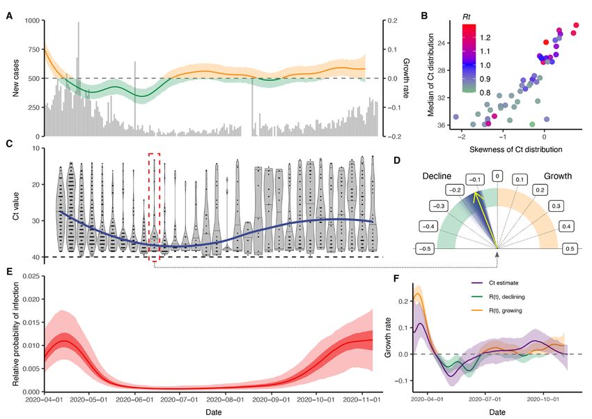
number of days between infection and sampling; and (2) the          for the epidemic trajectory up to and at that point in time
likelihood of being infected on a given day prior to the sample     (Fig. 2C). Note that the only facility-specific data for each of
date. For (1), we use a Bayesian model and define priors for        these fits were the Ct values and number of negative tests
the mode and range of Ct values following infection based on        from each single cross-sectional sample. Additional ancillary
the existing literature (Materials and Methods: Ct Value            information included prior distributions for the epidemic
Model and Single Cross-Section Model). For (2), we initially        seed time (after March 1) and the within-host virus kinetics.
develop two models to describe the probability of infection         To assess the fit, we compare the predicted Ct distribution
over time: (a) constant exponential growth of infection inci-       (Fig. 2B) and point prevalence (Fig. 2D) from each fit to the
dence; and (b) infections arising under an SEIR model. Both         data and compare the growth rates from these fits to the
models provide estimates for the epidemic growth rate but           baseline estimates. Posterior distributions of all Ct value
make different assumptions regarding the possible shape of          model parameters are shown in fig. S8.
the outbreak trajectory: the exponential growth model as-               While both sets of results are fitted models and so neither
sumes a constant growth rate over the preceding five weeks          can be considered the truth, we find that the Ct method fit to
and requires few prior assumptions, whereas the SEIR model          one cross-section of data provides a similar posterior median
assumes that the growth rate changes daily depending on the         trajectory to the baseline estimate, which required three sep-

                                                                                                                                         Downloaded from http://science.sciencemag.org/ on July 30, 2021
remaining number of susceptible individuals, but requires           arate point prevalences with near-universal testing at each
more prior information.                                             time point. In particular, the Ct-based models appear to ac-
    To demonstrate the potential of this method with a single       curately discern whether the samples were taken soon or long
cross-section from a closed population, we first investigate        after peak infection incidence. Both methods were in agree-
how the distribution of Ct values and prevalence of PCR pos-        ment over the direction of the past average and recent daily
itivity changed over time in four well-observed Massachusetts       growth rates (i.e., whether the epidemic is currently growing
long-term care facilities that underwent SARS-CoV-2 out-            or declining, and whether the growth rate has dropped rela-
breaks in March and April 2020 (29). In each facility, we have      tive to the past average). The average growth rate estimates
the results of near-universal PCR testing of residents and staff    were very similar between the prevalence-only and Ct value
from three time points after the outbreak began, including          models at most time points, though the daily growth rate ap-
the number of positive samples, the Ct values of positive sam-      peared to decline earlier in the prevalence-only compart-
ples, and the number of negative samples (Materials and             mental model. These estimates have a great deal of
Methods: Long-Term Care Facilities Data). To benchmark              variability, however, and should be interpreted in that con-
our Ct value-based estimates of the epidemic trajectory, we         text. This is especially clear in fig. S7, where the other facili-
first estimated the trajectory using a standard compart-            ties exhibit more variability between estimates from the two
mental modeling approach fit to the measured point preva-           methods. Overall, these results show that a single cross-sec-
lences over time in each facility (Fig. 2A). Specifically, we fit   tion of Ct values can provide similar information to point
a simple extended SEIR (SEEIRR) model, with additional ex-          prevalence estimates from three distinct sampling rounds,
posed and recovered compartments describing the duration            when the epidemic trajectory is constrained, as in a closed
of PCR positivity (Materials and Methods: Epidemic Trans-           population.
mission Models), to the three observed point prevalence val-            To ensure that our method provides accurate estimates of
ues from each facility. Because the testing was nearly              the full epidemic curve, we performed extensive simulation-
universal, this approach provides a near ground truth of the        recovery experiments using a synthetic closed population un-
epidemic trajectory against which we can evaluate the accu-         dergoing a stochastic SEIR epidemic. Figure S9 shows the re-
racy of the Ct value-based approaches. We call this the base-       sults of one such simulation, demonstrating the information
line estimate. Figure 2 shows results and data for one of the       gained from using a single cross-section of virological test
long-term care facilities, while figs. S6 and S7 show results for   data when attempting to estimate the true infection inci-
the other three.                                                    dence curve at different points during an outbreak. We assess
    As time passes, the distribution of observed Ct values at       performance using various simulations, including a version
each time point in the long-term care facilities (Fig. 2B) shifts   of the method that uses only positive Ct values without infor-
higher (lower viral loads) and becomes more left-skewed. We         mation on the fraction positive, simulations of different pop-
observed that these shifts tracked with the changing (i.e., de-     ulation sizes, and estimation using prior distributions of
clining) prevalence in the facilities. To assess if these changes   decreasing strengths; details are in Supplementary Materials:
in Ct value distributions indeed reflected underlying changes       Simulated Long-Term Care Facility Outbreaks and results in
in the epidemic growth rate, we fit the exponential growth          figs. S10 to S12.
and simple SEIR models using the Ct likelihood to each indi-            Although no real long-term care facility data were availa-
vidual cross-section of Ct values to get posterior distributions    ble to assess the method’s accuracy during the early phase of

First release: 3 June 2021                              www.sciencemag.org       (Page numbers not final at time of first release)   3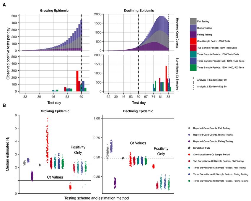
the epidemic outbreak, the simulation experiments reveal            random sampling schemes that increase or decrease over
that the method can be used at all stages of an epidemic. Fur-      time with test availability.
thermore, although there is a substantial uncertainty in the            To demonstrate the performance of these Ct-based meth-
growth rate estimates, these analyses show that a single-cross      ods, we simulate outbreaks under a variety of testing schemes
section of data can be used to determine whether the epi-           using SEIR-based simulations and sample Ct values from the
demic has been recently increasing or decreasing. The poste-        outbreaks (Materials and Methods: Simulated Testing
rior probability of growth versus decline can be used for this      Schemes). We compare the performance of Rt estimation us-
assessment, acting like a hypothesis test when the credible         ing reported case counts (based on the testing scheme) via
interval excludes zero or in a broader inferential way if it does   the R package EpiNow2 (32, 33), where reporting depends on
not. Although this is a trivial result for SARS-CoV-2 incidence     testing capacity and the symptom status of infected individ-
in many settings where cases, hospitalizations or deaths al-        uals, to the performance of our methods when one, two, or
ready provide a clear picture of epidemic growth or decline,        three surveillance samples are available with observed Ct val-
for locations and future outbreaks where testing capacity is        ues, with a total of about 0.3% of the population sampled
restricted, our results show that a single cross-sectional ran-     (3000 tests spread among the samples).
dom sample of a few hundred tested individuals combined                 Figure 3 plots the posterior median Rt from each of the

                                                                                                                                         Downloaded from http://science.sciencemag.org/ on July 30, 2021
with reasonable priors (for example, constraining the epi-          100 simulations of each method when the epidemic is grow-
demic seed time to within a one-to-two-month window) could          ing (day 60) and declining (day 88). Except when only one
be used to immediately estimate the stage of an outbreak.           sample is used, the Ct-based methods fitting to an SEIR
Moreover, this inferential method provides the basis for com-       model exhibit minimal bias, even when the number of tests
bining cross-sections for multiple testing days.                    substantially changes across sample days. For the single sam-
                                                                    ple estimates during the growth phase, the posterior median
Inferring the Epidemic Trajectory Using Multiple                    estimates are shifted above the true value because a range of
Cross-Sections                                                      R0 values are consistent with the data—the prior density for
While a single cross-section of Ct values can reasonably esti-      R0 is uniform between 1 and 10 with a median of 5.5, which
mate the trajectory of a simple outbreak represented by a           weights the posterior median higher than the true value.
compartmental model, more complex epidemic trajectories             Methods based on reported case counts, on the other hand,
will require more cross-sections for proper estimation. Here,       consistently exhibit noticeable upward bias when testing
we extend our method to combine data from multiple cross-           rates increase over the observed period and substantial
sections, allowing us to estimate the full epidemic trajectory      downward bias when testing rates decrease. The Ct-based
more reliably (Materials and Methods: Multiple Cross-Sec-           methods do exhibit higher variability, however. This is cap-
tions Model and Markov Chain Monte Carlo Framework). In             tured by the Bayesian inference model, as all of the Ct-based
many settings, the epidemic trajectory is monitored using re-       methods achieve at least nominal coverage of the 95% credi-
ported case counts. Limiting reported cases to those with pos-      ble intervals among these 100 simulations (fig. S13).
itive test results, the daily number of new positives can be            An alternative approach to estimating Rt using case
used to calculate Rt (3). However, this approach can be ob-         counts is to fit a standard compartmental model to the ob-
scured when the definition of a case changes during the             served proportion of positive tests from a random sample. To
course of an epidemic (30). Furthermore, such data often rep-       demonstrate the value of incorporating Ct values rather than
resent the growth rate of positive tests, which can change dra-     simply using positivity rates from a surveillance sample, we
matically based on changing test capacity rather than the           also compare the results to an SEIR model fit to point preva-
incidence of infection, requiring careful monitoring and ad-        lence observed at the same sample times, assuming PCR pos-
justments to account for changes in testing capacity, the de-       itivity represents the infectious stage of the disease. In this
lay between infection and test report date, and the conversion      alternate method, this misspecification of the SEIR model re-
from prevalence to incidence. Death counts are also used to         sults in inaccurate Rt estimates during the decline phase of
estimate the epidemic trajectory, but these are substantially       the simulation (Fig. 3B). While a more accurate model might
delayed and the relationship between cases and deaths is not        distinguish the infectious stage and duration of PCR positiv-
stable (31). When, instead, Ct values from surveillance sam-        ity, as in the SEEIRR model, this simple model represents an
pling are available, our methods can overcome these limita-         approach that might be used to infer incidence changes from
tions by providing a direct mapping between the distribution        prevalence data in the absence of a quantified relationship
of Ct values and infection incidence. While case count meth-        between infection state and PCR positivity.
ods exhibit bias due to changing test rates (5), our method             We also assessed the precision of our estimates using
provides a means to estimate Rt using only one or a few sur-        smaller sample sizes and different deployment of tests among
veillance samples, and this method can accommodate                  testing days for a given sample size. These comparisons are

First release: 3 June 2021                              www.sciencemag.org       (Page numbers not final at time of first release)   4
shown in fig. S13, which also compares the Ct-based method The median Ct value rose (corresponding to a decline in me-
to the positivity-based estimation. The Ct-based method per- dian viral load) and skewness of the Ct distribution fell in the
forms well in many cases with sample sizes as low as 200– late spring and early summer, as shelter-in-place orders and
500 tests. When testing is stable, reported case counts pro- other non-pharmaceutical interventions were rolled out (Fig.
vide a more precise estimate of the trajectory. However, a 4C), but the median declined and skewness rose in late sum-
small number of tests (e.g., the same number of tests as used mer and early fall as these measures were relaxed, coinciding
for one day of routine case detection) devoted to two or three with an increase in observed case counts for the state (Fig.
surveillance samples can provide unbiased estimation when 4A).
reported case counts may be biased. Using the observed Ct values, we estimated the daily
growth rate of infections using the SEIR model on single
Reconstructing Complex Incidence Curves Using Ct cross-sections (Fig. 4D and figs. S14 and S15) and the full ep-
Values idemic trajectory using the GP model (Fig. 4E and fig. S16).
Simple epidemic models are useful to understand recent in- Similar temporal trends were inferred under both models
cidence trends when data are sparse or in relatively closed (fig. S17), and the GP model provided growth rate estimates
populations where the epidemic start time is approximately that followed those estimated using observed case counts
Downloaded from http://science.sciencemag.org/ on July 30, 2021
known (Supplementary Materials: Epidemic Seed Time Pri- (Fig. 4F). While these data are not strictly a random sample
ors). In reality, however, the epidemic usually follows a more of the community, and the observed case counts do not nec-
complex trajectory which is difficult to model parametrically. essarily provide a ground truth for the Rt value, these results
For example, the SEIR model does not account for the imple- demonstrate the ability of this method to re-create epidemic
mentation/relaxation of non-pharmaceutical interventions trajectories and estimate growth or decline of cases using
and behavior changes that affect pathogen transmission un- only positive Ct values collected through routine testing. We
less explicitly specified in the model. For a more flexible ap- assessed the robustness of the estimated GP trajectory to
proach to estimating the epidemic trajectory from multiple smaller sample sizes by refitting the model after subsampling
cross-sections, we developed a third model for infection inci- different numbers of Ct values from the dataset (fig. S18). In-
dence, using a Gaussian process (GP) prior for the underlying terestingly, our estimated epidemic trajectory using only rou-
daily probabilities of infection (34). The GP method provides tinely generated Ct values from a single hospital was
estimated daily infection probabilities without making strong remarkably correlated with changes in community-level viral
assumptions about the epidemic trajectory, assuming only loads obtained from wastewater data (fig. S19) (35).
that infection probabilities on contemporaneous days are
correlated, with decreasing correlation at increasing tem- Discussion
poral distances (Supplementary Materials: Epidemic Trans- The usefulness of Ct values for public health decision making
mission Models). Movie S1 demonstrates how estimates of is currently the subject of much discussion and debate. One
the full epidemic trajectory, representing a simulation for the unexplained observation which has been consistently ob-
implementation and subsequent relaxation of non-pharma- served in many locations is that the distribution of observed
ceutical interventions, can be sequentially updated using this Ct values has varied over the course of the current SARS-CoV-
model as new samples become available over time. Movie S2 2 pandemic, which has led to questions over whether the fit-
shows how the precision of the estimated epidemic curve de- ness of the virus has changed (12, 14, 16). Our results demon-
creases at smaller sample sizes, where 200 samples per week strate that this can be explained as an epidemiologic
were sufficient to reliably track the epidemic curve. Movie S3 phenomenon, without invoking any change in individual-
shows how estimation remains accurate if sampling is only level viral kinetics or testing practices. This method alone,
initiated partway through the epidemic. however, cannot prove that is the case for any specific setting,
With the objective of reconstructing the entire incidence as changing viral properties or changes in test availability
curve using routinely collected RT-qPCR data, we used anon- may also lead to such shifts in Ct value distributions. We find
ymized Ct values from positive samples measured from near- that properties of the population-level Ct distribution
universal testing of all hospital admissions and non-admitted strongly correlate with estimates for the effective reproduc-
ER patients in the Brigham and Women’s Hospital (BWH) in tive number or growth rate in real-world settings, in line with
Boston, MA, between April 15 and November 10, 2020 (Mate- our theoretical predictions.
rials and Methods: Brigham and Women’s Hospital Data). We Using quantitative diagnostic test results from multiple
aligned these with estimates for Rt based on case counts in different tests conducted in a single cross-sectional survey,
Massachusetts (Fig. 4, A to C). The median and skewness of epidemic trends have previously been inferred from virologi-
the detectable Ct distribution was correlated with Rt (Fig. 4B), cal data (18). The methods we describe here use the phenom-
in line with our theoretical predictions (depicted in Fig. 1). enon observed in the present pandemic and the relationship
First release: 3 June 2021 www.sciencemag.org (Page numbers not final at time of first release) 5between incidence rate, time since infection, and virologic variants (39, 40). When samples are obtained through popu-
test results to estimate a community’s position in the epi- lation-wide testing, an association between lower Ct values
demic curve, under various models of epidemic trajectories, and emerging variants can be partially explained by those
based on data from one or more cross-sectional surveys using variants having a higher growth rate with a preponderance
a single virologic test. Comparisons of simulated Ct values of recent infections compared to pre-existing, declining vari-
and observed Ct values with growth rates and Rt estimates ants. For example, a recent analysis of Ct values from P.1 and
validate this general approach. Despite the challenges of sam- non-P.1 variant samples in Manaus, Brazil initially found that
pling variability, individual-level differences in viral kinetics, P.1 samples had significantly lower Ct values (41). However,
and the limitations of comparing results from different labor- after accounting for the time between symptom onset and
atories or instruments, our results demonstrate that RT- sample collection date (where shorter delays should lead to
qPCR Ct values, with all of their variability for an individual, lower Ct values), the significance of this difference was lost.
can be highly informative of population-level dynamics. This We caution that this finding does not exclude the possibility
information is lost when measurements are reduced to binary of newer variants causing infections with higher viral loads;
positive or negative classifications, as has been the case rather, it highlights the need for lines of evidence other than
through most of the SARS-CoV-2 pandemic. surveillance testing data.
Downloaded from http://science.sciencemag.org/ on July 30, 2021
Here, we focused on the case of randomly sampling indi- These results are sensitive to the true distribution of ob-
viduals from the population. This method will therefore be served viral loads each day after infection. Different swab
most useful in settings where representative surveillance types, sample types, instruments, or Ct thresholds may alter
samples can be obtained independently of COVID-19 symp- the variability in the Ct distribution (15, 16, 42, 43), leading to
toms, such as the REACT study in England (36). Even rela- different relationships between the specific Ct distribution
tively small cross-sectional surveys, for example in a given and the epidemic trajectory. Where possible, setting-specific
city, may be very useful for understanding the direction that calibrations, for example based on a reference range of Ct val-
an outbreak is heading. Standardized data collection and ues, will help to generate precise estimates. This method will
management across regions, along with wider use of random be most useful in cases where the population-level viral load
sampling, would further improve the usefulness of these kinetics can be estimated, either through direct validation or
methods, which demonstrate another use case for such sur- by comparison with a reference standard, for the instruments
veillance (37, 38). These methods allow municipalities to eval- and samples used in testing. Here, we generated a viral kinet-
uate and monitor, in real-time, the role of various epidemic ics model based on observed properties of measured viral
mitigation interventions, for example by conducting even a loads in the literature (proportion detectable over time fol-
single or a small number of random virologic testing samples lowing symptom onset, distribution of Ct values from positive
as part of surveillance rather than simply relying on routine specimens) and used these results to inform priors on key pa-
testing results. rameters when estimating growth rates. The growth rate es-
Extrapolation of these findings to Ct values obtained timates can therefore be improved by choosing more precise,
through strategies other than a population census or a mostly accurate priors relevant to the observations used during
random sample requires additional considerations. When model fitting. In cases where results come from multiple test-
testing is based primarily on the presence of symptoms or ing platforms, the model should either be adjusted to account
contact tracing efforts, infected individuals are more likely to for this by specifying a different distribution for each plat-
be sampled at specific times since infection, which will im- form based on its properties or, if possible, the Ct values
pact the distribution of measured Ct values. Further compli- should be transformed to a common scale such as log viral
cations arise when the delay between infection or symptom copies. If these features of the tests change substantially over
onset and sample collection changes over the course of the time, results incorporating multiple cross-sections might ex-
epidemic, for example because of a strain on testing capacity. hibit bias and will not be reliable.
Nonetheless, our simulation results suggest that the epidemic Results could also be improved if individual-level features
trajectory can still influence Ct values measured under symp- that may affect viral load, such as symptom status, age, and
tom-based surveillance, though the strength of this associa- antiviral treatment, are available with the data and incorpo-
tion will depend on a number of additional considerations as rated into the Ct value model (14–16, 44, 45). A similar ap-
described in fig. S4. Additional work is needed to extend the proach may also be possible using serologic surveys, as an
inference methods presented here to use non-random surveil- extension of work that relates time since infection to anti-
lance samples. body titers for other infectious diseases (27, 28). If multiple
The overall finding of a link between epidemic growth types of tests (e.g., antigen and PCR) are conducted at the
rates and measured Ct distributions is important for inter- same time, combining information could substantially reduce
preting virologic data in light of emerging SARS-CoV-2 uncertainty in these estimates (18). If variant strains are
First release: 3 June 2021 www.sciencemag.org (Page numbers not final at time of first release) 6associated with different viral load kinetics and become com- provides information on underlying viral dynamics. Although
mon (40, 46), this should be incorporated into the model as there are challenges to relying on single Ct values for individ-
well. Other features of the pathogen, such as the relationship ual-level decision making, the aggregation of many such
between the viral loads of infector and infectee, might also measurements from a population contains substantial infor-
affect population-level variability over time. Using virologic mation. These results demonstrate how one or a small num-
data as a source of surveillance information will require in- ber of random virologic surveys can be best used for epidemic
vestment in better understanding Ct value distributions as monitoring. Overall, population-level distributions of Ct val-
new instruments and techniques come online and as variants ues, and quantitative virologic data in general, can provide
emerge, and in rapidly characterizing these distributions for information on important epidemiologic questions of inter-
future emerging infectious diseases. Remaining uncertainty est, even from a single cross-sectional survey. Better epidemic
can be incorporated into the Bayesian prior distribution. planning and more targeted epidemiological measures can
This method has several limitations. While the Bayesian then be implemented based on such a survey, or Ct values can
framework incorporates the uncertainty in viral load distri- be combined across repeated samples to maximize the use of
butions into inference on the growth rate, parametric as- available evidence.
sumptions and reasonably strong priors on these
Downloaded from http://science.sciencemag.org/ on July 30, 2021
distributions aid in identifiability. If these parametric as- Materials and Methods
sumptions are violated, for example when SEIR models are
Long-Term Care Facilities Data
used across time periods when interventions likely affected
Data from Massachusetts long-term care facilities were naso-
transmission rates, inference may not be reliable. In addition,
pharyngeal specimens collected from staff and residents pro-
the methods described here and the relationship between in-
cessed at the Broad Institute of MIT and Harvard CRSP CLIA
cidence and skewness of Ct distributions become less reliable
laboratory, with an FDA Emergency Use Authorized labora-
when there are very few positive cases, so results should be
tory-developed assay. Ct values for N1 and N2 gene targets
interpreted with caution and sample sizes increased in peri-
were provided along with sample collection date, a random
ods with low incidence. In some cases, with one or a small
tube ID, and a unique anonymized institute ID to reflect that
number of cross-sections, the observed Ct distribution could
specimens came from distinct institutions. The specimens
plausibly result from all individuals very early in their infec-
used here originated in early 2020 when public health efforts
tion at the start of fast epidemic growth, all during the recov-
in Massachusetts led to comprehensively serial testing senior
ery phase of their infection during epidemic decline, or a
nursing facilities as described previously (29). Swabs from
mixture of both (Fig. 4E and fig. S15). We therefore used a
those public health efforts were processed for clinical diag-
parallel tempering Markov chain Monte Carlo (MCMC) algo-
nostics. Sample collection dates ranged from April 6, 2020, to
rithm for the single cross-section estimates, which can accu-
May 5, 2020, with each facility undergoing three sampling
rately estimate these multimodal posterior distributions (47).
rounds. Each round took a median of 2 days (range 1–6 days)
Interpretation of the estimated median growth rate and cred-
to complete. The anonymized Ct data was made available,
ible intervals should be done with proper epidemiological
and the N2 Ct values were used for these analyses. For all
context: estimated growth rates that are grossly incompatible
analyses presented here, sample collection dates were
with other data can be safely excluded.
grouped into sampling rounds and analyzed based on the
This method may also overstate uncertainty in the viral
mean collection date for that round (i.e., the dates shown in
load distributions if results from different machines or pro-
Fig. 2 and figs. S6 and S7).
tocols are used simultaneously to inform the prior. A more
precise understanding of the viral load kinetics—in particu-
Brigham and Women’s Hospital Data
lar, modeling these kinetics in a way that accounts for the
Data from the Brigham and Women’s Hospital in Boston,
epidemiologic and technical setting of the measurements—
Massachusetts, were nasopharyngeal specimens from pa-
will help improve this approach and determine whether Ct
tients processed on a Hologic Panther Fusion SARS-CoV-2 as-
distribution parameters from different settings are compara-
say. Ct values for the ORF1ab gene were provided alongside
ble. Because of this, semiquantitative measures from RT-
sample collection date, with collection dates ranging from
qPCR should be reported regularly for SARS-CoV-2 cases and
April 3, 2020, to November 10, 2020. For these analyses, we
early assessment of pathogen load kinetics should be a prior-
grouped samples by week of collection on the epidemiological
ity for future emerging pathogens. The use of control meas-
calendar and used the mid-point of each week for the anal-
urements, like using the ratio of detected viral RNA to
yses shown in Fig. 4. Testing during the first two weeks in
detected human RNA, could also improve the reliability and
April 2020 was restricted to patients with symptoms con-
comparability of Ct measures.
sistent with COVID-19 and who needed hospital admission.
The Ct value is a measurement with magnitude, which
Following April 15, testing criteria for this platform were
First release: 3 June 2021 www.sciencemag.org (Page numbers not final at time of first release) 7expanded to include all asymptomatic hospital admissions, in the population-level distribution and not individual trajec-
symptomatic patients in the emergency room who were not tories, we assumed that observed Ct values a days after infec-
admitted to the hospital, and inpatients requiring testing tion, C(a), followed a Gumbel distribution with location
who were not in labor. Symptomatic ER patients who were (mode) parameter Cmode(a) and scale parameter σ(a) that also
admitted to the hospital were tested on a different PCR plat- may depend on the number of days a after infection. We
form and are not considered here. In the analyses presented chose a Gumbel distribution to capture overdispersion of
here, we use only samples taken after April 15. While this is high measured Ct values. This distribution captures the vari-
not a perfectly representative surveillance sample, the rou- ation resulting from both swabbing variability and individ-
tine testing of hospital admissions who were not seeking ual-level differences in viral kinetics. We note that at any
COVID treatment creates a cohort that is less biased than point in the infection, there is a considerable amount of per-
symptom-based testing and represents the overall rise and son-to-person and swab-to-swab variation in viral loads (50–
fall of cases in the hospital’s catchment area. Daily data are 52), including a possible difference by symptom status (15, 53,
aggregated by week. Daily confirmed case counts for Massa- 54). Tracking individual-level viral kinetics would require a
chusetts were obtained from The New York Times, based on hierarchical model capturing individual-level parameters,
reports from state and local health agencies (48). but is not necessary for this analysis.
Downloaded from http://science.sciencemag.org/ on July 30, 2021
The rationale behind this parameterization and the cho-
Epidemic Transmission Models sen parameter values is discussed in Supplementary Materi-
Throughout these analyses, we used four mathematical mod- als: Selecting Viral Kinetics and Compartmental Model
els to describe daily SARS-CoV-2 transmission over the course Parameters. We note that in all analyses, we used informative
of an epidemic. Full model descriptions are given in Supple- priors for key features of viral load kinetics rather than fixing
mentary Materials: Epidemic Transmission Models, and a point estimates, incorporating uncertainty into our inference.
brief overview is provided here in order of introduction in the The process for generating these priors is described in Sup-
main text. First, the SEIR Model is a compartmental model plementary Materials: Informing the Viral Kinetics Model.
which assumes that the growth rate of new infections de- We performed this calibration step separately for the long-
pends on the current prevalence of infectious and susceptible term care facility and BWH datasets, as the gene targets and
individuals by modeling the proportion of the population testing platform were different, and thus Ct values are not
who are susceptible, exposed, infected, or recovered with re- directly comparable.
spect to disease over time. Second, the Exponential Growth
Model assumes that new infections arise under a constant ex- Relationship Between Observed Ct Values and Daily
ponential growth rate. Third, the SEEIRR Model is a modifi- Probability of Infection
cation of the SEIR model with additional compartments for Single Cross-Section Model
individuals who are exposed but not yet detectable by PCR For a single testing day t, let π t − Amax ,..., π t −1 be the marginal
and individuals who are recovered but still detectable by PCR. daily probabilities of infection for the whole population for
Finally, the Gaussian Process Model describes the epidemic
Amax days to 1 day prior to t, respectively, where t − Amax is the
trajectory as a vector of daily infection probabilities, where a
earliest day of infection that would result in detectable PCR
Gaussian process prior is used to ensure that daily infection
values on the testing day. That is, πt − a is the probability that
probabilities are correlated in time; days that are chronolog-
a randomly-selected individual in the population was in-
ically close in time are more correlated than those that are
chronologically distant. fected on day t − a. Let pa(x) be the probability that the Ct
value is x for a test conducted a days after infection given
Ct Value Model that the value is detectable (i.e., the Gumbel probability den-
We developed a mathematical model describing the distribu- sity function normalized to the observable values). Then pa(x)
tion of observed SARS-CoV-2 viral loads over time following = P[C(a) = x]/P[0 ≤ C(a) < CLOD], where P[C(a) = x] is the
infection. The model is described in full in Supplementary Gumbel probability density function with location parameter
Materials: Ct Value Model. This model is similar to that used Cmode(a) and scale parameter σ(a). Let φa be the probability
by Larremore et al. (49), but allows for more flexibility in the of a Ct value being detectable a days after infection, which
decline of viral load during recovery. We used a parametric depends on C(a) and any additional decline in detectability.
model describing the modal Ct value, Cmode(a), for an individ- Let the PCR test results from a sample of n individuals be
ual a days after infection, represented by the solid black line recorded as X1,…,Xn. Then, for xi < CLOD (i.e., a detectable Ct
in fig. S1B. The measured Ct value is a linear function of the value), the probability of individual i having Ct value xi is
log of the viral load in the sample, but we describe the model given by:
on the Ct scale to match the data. Because we are interested
First release: 3 June 2021 www.sciencemag.org (Page numbers not final at time of first release) 8= (
i π t − Amax ,..., π t −1
P X i x= ) ∑ p ( x )φ π
Amax
a i a t −a
(
X 1t1 ,..., X nt11 ,..., X ntTT {π t } )
I ( X i j < CLOD ) ( )
a =1
T
nj
( ( ) ) ( )
t t
I X i j ≥ CLOD
The probability of a randomly chosen individual being detect- ∏ ∏ i =1 ∑ a 1 =pa X i φ a π t j − a 1 − ∑ a max1 φaπ t j − a
Amax A
=
tj
=
able to PCR on testing day t is:
j =1
( ) I ( X i j < CLOD )
Amax
n j n−j
∑ φa π t − a ( ( ) ) 1 − ∑ Amax φaπ t − a
t
P X i < CLOD π t − Amax ,..., π t −1 =
T
∏ ∏ ∑ φ π
Amax
=
tj
a =1 = i =1 a 1=
p a X i a t − a
a 1
j =1
j j
So the likelihood for the n PCR values is given by:
−
(
X 1 ,..., X n π t − Amax ,..., π t − a ) where n j is the number of undetectable samples on testing
day tj.
( ) ( )
I ( X i < CLOD ) I ( X i < CLOD )
n
Only considering samples with a detectable Ct value gives
∏ ∑ a 1= pa ( X i ) φ a π t − a 1 − ∑ a 1 φa π t − a
Amax Amax
the likelihood:
i =1
where I ( ⋅) equals 1 if the interior statement is true and 0 if n j Amax p X t j φ π
( )
∏ i =1 ∑ a =1 a i a t j − a
( )
T
it is false. X 1 ,..., X n1 ,..., X nT {π t } = ∏
t1 t1 tT
nj
j =1 ∑ Amax φaπ t − a
Downloaded from http://science.sciencemag.org/ on July 30, 2021
If only detectable Ct values are recorded as X1,…,Xn, then
a =1 j
the likelihood function is given by:
Either of these likelihoods can be parameterized using the
(
X 1 ,..., X n π t − Amax ,..., π t −1 ) exponential growth rate model described above. However,
the exponential growth rate model is less likely to be a good
∑ ∏ i =1 ∑ a max pa ( X i ) φaπ t − a
n A
n ( ) φ π
Amax
p X approximation of the true incidence probabilities over a
∏
− =
a =1 A
1
=
a i a t a
i =1 ∑ a =1 φaπ t − a ( ) longer period of time, so it may not be a good model for mul-
n
∑ a max=1 φaπ t − a
max A
tiple test days that cover a long stretch of time.
Either of these likelihoods can be maximized to get nonpara- The multiple cross-section likelihood is primarily used to
metric estimates of the daily probability of infection, with the fit the Gaussian Process model, estimating the daily probabil-
constraint that ∑ a max π t − a ≤ 1 . To improve power and inter- ity of infection, {πt}, conditional on the set of observed Ct val-
A
=1
ues. (See Supplementary Materials: Parametric Models for
pretability of the estimates, however, we consider two para- Fitting Cross-Sectional Viral Load Data). The SEIR model can
metric models based on the epidemic transmission models be used with multiple testing days as well. It is fit as de-
described above: (i) a model assuming exponential growth of scribed for the single cross-section model, but with one of
infection incidence over a defined period prior to the sam- these likelihoods in place of the single cross-section model
pling day; and (ii) an SEIR compartmental model in a closed likelihood, with posterior distribution estimates obtained via
finite population, where the basic reproduction number R0 is MCMC fitting.
a parameter estimated by the model but does not vary over
time (i.e., there are no interventions that reduce transmissi- Markov Chain Monte Carlo Framework
bility). See Supplementary Materials: Parametric Models for All models, including those using Ct values (SEIR Model, Ex-
Fitting Cross-Sectional Viral Load Data for details of the like- ponential Growth Model and the Gaussian Process Model)
lihoods used in these methods. and those using only prevalence (SEIR Model, SEEIRR Model)
were fitted using a Markov chain Monte Carlo framework. We
Multiple Cross-Sections Model used a Metropolis-Hastings algorithm to generate either mul-
Now we consider settings where there are multiple days of tivariate Gaussian or univariate uniform proposals. For all
testing, t1,…,tT. We again denote by πt the probability of infec- single-cross section analyses (Figs. 2 and 3), we used a modi-
tion on day t and now denote the sampled Ct value for the ith fied version of this framework with parallel tempering: an
individual sampled on test day tj by X i j , where i ∈ 1,…,nj for
t
extension of the algorithm that uses multiple parallel chains
test day j and j ∈ 1,…,T. Note that individual i may refer to to improve sampling of multimodal posterior distributions
different individuals on different testing days. Let {πt} be the (47). For the multiple cross section analyses including those
daily probabilities of infection for any day t where an infec- in Fig. 4, we used the unmodified Metropolis-Hastings algo-
tion on day t could be detectable using a PCR test on one of rithm because the computational time of the parallel temper-
the testing days. By a straightforward extension of the likeli- ing algorithm is far longer, and these analyses were
hood for the single cross-section model, the nonparametric underpinned by more data and less affected by multimodal-
likelihood for the set of infection probabilities {πt}, when ity. In all analyses, three chains were run upward of 80,000
samples with and without a detectable Ct value are included, iterations (500,000 iterations for the Gaussian process mod-
is given by: els). Convergence was assessed based on all estimated
First release: 3 June 2021 www.sciencemag.org (Page numbers not final at time of first release) 9parameters having an effective sample size greater than 200 4. M. Lipsitch, D. L. Swerdlow, L. Finelli, Defining the epidemiology of COVID-19—
( R̂ )
Studies needed. N. Engl. J. Med. 382, 1194–1196 (2020).
and a potential scale reduction factor of less than 1.1, doi:10.1056/NEJMp2002125 Medline
5. R. A. Betensky, Y. Feng, Accounting for incomplete testing in the estimation of
evaluated using the coda R package (55). All assumed prior epidemic parameters. Int. J. Epidemiol. 49, 1419–1426 (2020).
distributions are described in table S1. doi:10.1093/ije/dyaa116 Medline
6. J. L. Vaerman, P. Saussoy, I. Ingargiola, Evaluation of real-time PCR data. J. Biol.
Simulated Data Regul. Homeost. Agents 18, 212–214 (2004). Medline
7. M. R. Tom, M. J. Mina, To interpret the SARS-CoV-2 test, consider the cycle
All simulated data were generated under the same frame- threshold value. Clin. Infect. Dis. 71, 2252–2254 (2020). doi:10.1093/cid/ciaa619
work but with different models and assumptions for the un- Medline
derlying epidemic trajectory. For each simulation, data were 8. T. C. Quinn, M. J. Wawer, N. Sewankambo, D. Serwadda, C. Li, F. Wabwire-Mangen,
generated in four steps: 1) the daily probability of transmis- M. O. Meehan, T. Lutalo, R. H. Gray, Rakai Project Study Group, Viral load and
heterosexual transmission of human immunodeficiency virus type 1. N. Engl. J.
sion, {πt}, is calculated using either a deterministic SEIR, a Med. 342, 921–929 (2000). doi:10.1056/NEJM200003303421303 Medline
stochastic SEIR model, or a Gaussian Process model; 2) On 9. J. A. Fuller, M. K. Njenga, G. Bigogo, B. Aura, M. O. Ope, L. Nderitu, L. Wakhule, D. D.
each day of the simulation, new infections are simulated un- Erdman, R. F. Breiman, D. R. Feikin, Association of the CT values of real-time PCR
der the model It ~ Binomial(N, πt), where N is the population of viral upper respiratory tract infection with clinical severity, Kenya. J. Med. Virol.
85, 924–932 (2013). doi:10.1002/jmv.23455 Medline
Downloaded from http://science.sciencemag.org/ on July 30, 2021
size of the simulation and It is the number of new infections 10. S. Bolotin, S. L. Deeks, A. Marchand-Austin, H. Rilkoff, V. Dang, R. Walton, A.
on day t (all other individuals are assumed to have escaped Hashim, D. Farrell, N. S. Crowcroft, Correlation of Real Time PCR Cycle Threshold
infection); 3) A subset of individuals are sampled on particu- Cut-Off with Bordetella pertussis Clinical Severity. PLOS ONE 10, e0133209
lar days of the simulation determined by the testing schemes (2015). doi:10.1371/journal.pone.0133209 Medline
11. T. K. Tsang, B. J. Cowling, V. J. Fang, K. H. Chan, D. K. M. Ip, G. M. Leung, J. S. M.
described below and in Supplementary Materials: Compari- Peiris, S. Cauchemez, Influenza A virus shedding and infectivity in households. J.
son of Analysis Methods; 4) For each individual sampled on Infect. Dis. 212, 1420–1428 (2015). doi:10.1093/infdis/jiv225 Medline
day u, a Ct value was simulated under the model Xi ~ Gum- 12. M. Moraz, D. Jacot, M. Papadimitriou-Olivgeris, L. Senn, G. Greub, K. Jaton, O.
Opota, Universal admission screening strategy for COVID-19 highlighted the
bel(Cmode(u − tinf), σ(u − tinf)), where tinf is the time of infection clinical importance of reporting SARS-CoV-2 viral loads. New Microbes New Infect.
for individual i. Cmode(u − t) and σ(u − t) are described in Sup- 38, 100820 (2020). doi:10.1016/j.nmni.2020.100820 Medline
plementary Materials: Ct Value Model. 13. Y. Chen, L. Li, SARS-CoV-2: Virus dynamics and host response. Lancet Infect. Dis.
20, 515–516 (2020). doi:10.1016/S1473-3099(20)30235-8 Medline
14. D. Jacot, G. Greub, K. Jaton, O. Opota, Viral load of SARS-CoV-2 across patients
Simulated Testing Schemes and compared to other respiratory viruses. Microbes Infect. 22, 617–621 (2020).
Standard approaches to estimating doubling time, growth doi:10.1016/j.micinf.2020.08.004 Medline
rate, or Rt are subject to misestimation as a result of changes 15. K. A. Walsh, K. Jordan, B. Clyne, D. Rohde, L. Drummond, P. Byrne, S. Ahern, P. G.
in testing policies (5). To assess the effect of such changes on Carty, K. K. O’Brien, E. O’Murchu, M. O’Neill, S. M. Smith, M. Ryan, P. Harrington,
SARS-CoV-2 detection, viral load and infectivity over the course of an infection. J.
our methods, we simulate changes in testing rates and assess Infect. 81, 357–371 (2020). doi:10.1016/j.jinf.2020.06.067 Medline
the effect on several methods for Rt estimation: using Epi- 16. A. S. Walker, E. Pritchard, T. House, J. V. Robotham, P. J. Birrell, I. Bell, J. I. Bell, J.
Now2 with reported case counts (33), using Ct-based methods N. Newton, J. Farrar, I. Diamond, R. Studley, J. Hay, K.-D. Vihta, T. Peto, N.
with random surveillance samples, and using PCR test posi- Stoesser, P. C. Matthews, D. W. Eyre, K. B. Pouwels, COVID-19 Infection Survey
Team, Ct threshold values, a proxy for viral load in community SARS-CoV-2 cases,
tivity alone with surveillance samples. We test these methods demonstrate wide variation across populations and over time. medRxiv
at two periods of an outbreak: once when the epidemic is ris- 2020.10.25.20219048 [Preprint]. 4 April 2021.
ing and once when it is falling. For the random samples for https://doi.org/10.1101/2020.10.25.20219048.
each of these analysis time points, we test from one to three 17. M. Gousseff, P. Penot, L. Gallay, D. Batisse, N. Benech, K. Bouiller, R. Collarino, A.
Conrad, D. Slama, C. Joseph, A. Lemaignen, F.-X. Lescure, B. Levy, M. Mahevas,
days of sampling for virologic testing with varying sample B. Pozzetto, N. Vignier, B. Wyplosz, D. Salmon, F. Goehringer, E. Botelho-Nevers,
sizes across the test days. Results are shown in Fig. 3 and fig. COCOREC study group, Clinical recurrences of COVID-19 symptoms after
S13; more details are in the Supplementary Materials: Com- recovery: Viral relapse, reinfection or inflammatory rebound? J. Infect. 81, 816–
parison of Analysis Methods. 846 (2020). doi:10.1016/j.jinf.2020.06.073 Medline
18. G. Rydevik, G. T. Innocent, G. Marion, R. S. Davidson, P. C. L. White, C. Billinis, P.
REFERENCES AND NOTES Barrow, P. P. C. Mertens, D. Gavier-Widén, M. R. Hutchings, Using combined
diagnostic test results to hindcast trends of infection from cross-sectional data.
1. H. V. Fineberg, M. E. Wilson, Epidemic science in real time. Science 324, 987 (2009).
PLOS Comput. Biol. 12, e1004901 (2016). doi:10.1371/journal.pcbi.1004901
doi:10.1126/science.1176297 Medline
Medline
2. World Health Organization, Public health surveillance for COVID-19: Interim
19. N. Keyfitz, Applied Mathematical Demography (Springer, ed. 2, 1985).
guidance (2020); www.who.int/publications/i/item/who-2019-nCoV-
20. J. Wallinga, M. Lipsitch, How generation intervals shape the relationship between
surveillanceguidance-2020.8.
growth rates and reproductive numbers. Proc. R. Soc. B. 274, 599–604 (2007).
3. T. Jombart, K. van Zandvoort, T. W. Russell, C. I. Jarvis, A. Gimma, S. Abbott, S.
doi:10.1098/rspb.2006.3754 Medline
Clifford, S. Funk, H. Gibbs, Y. Liu, C. A. B. Pearson, N. I. Bosse, Centre for the
21. B. Borremans, N. Hens, P. Beutels, H. Leirs, J. Reijniers, Estimating time of
Mathematical Modelling of Infectious Diseases COVID-19 Working Group, R. M.
infection using prior serological and individual information can greatly improve
Eggo, A. J. Kucharski, W. J. Edmunds, Inferring the number of COVID-19 cases
incidence estimation of human and wildlife infections. PLOS Comput. Biol. 12,
from recently reported deaths. Wellcome Open Res. 5, 78 (2020).
e1004882 (2016). doi:10.1371/journal.pcbi.1004882 Medline
doi:10.12688/wellcomeopenres.15786.1
First release: 3 June 2021 www.sciencemag.org (Page numbers not final at time of first release) 10You can also read