Year-long, broad-band, microwave backscatter observations of an alpine meadow over the Tibetan Plateau with a ground-based scatterometer
←
→
Page content transcription
If your browser does not render page correctly, please read the page content below
Earth Syst. Sci. Data, 13, 2819–2856, 2021
https://doi.org/10.5194/essd-13-2819-2021
© Author(s) 2021. This work is distributed under
the Creative Commons Attribution 4.0 License.

              Year-long, broad-band, microwave backscatter
            observations of an alpine meadow over the Tibetan
               Plateau with a ground-based scatterometer
          Jan G. Hofste1 , Rogier van der Velde1 , Jun Wen2 , Xin Wang3 , Zuoliang Wang3 , Donghai Zheng4 ,
                                      Christiaan van der Tol1 , and Zhongbo Su1
                             1 Facultyof Geo-Information Science and Earth Observation (ITC),
                                      University of Twente, Enschede, the Netherlands
      2 College of Atmospheric Sciences, Plateau Atmosphere and Environment Key Laboratory of Sichuan Province,

                              Chengdu University of Information Technology, Chengdu, China
        3 Key laboratory of Land Surface Process and Climate Change in Cold and Arid Regions, Northwest Institute

                    of Eco-Environment and Resources, Chinese Academy of Sciences, Lanzhou, China
                        4 National Tibetan Plateau Data Center, Institute of Tibetan Plateau Research,

                                        Chinese Academy of Sciences, Beijing, China
                                  Correspondence: Jan G. Hofste (j.g.hofste@utwente.nl)

                                 Received: 19 February 2020 – Discussion started: 11 March 2020
                            Revised: 19 April 2021 – Accepted: 12 May 2021 – Published: 16 June 2021

      Abstract. A ground-based scatterometer was installed on an alpine meadow over the Tibetan Plateau to study
      the soil moisture and temperature dynamics of the top soil layer and air–soil interface during the period Au-
      gust 2017–August 2018. The deployed system measured the amplitude and phase of the ground surface radar
      return at hourly and half-hourly intervals over 1–10 GHz in the four linear polarization combinations (vv, hh, hv,
      vh). In this paper we describe the developed scatterometer system, gathered datasets, retrieval method for the
      backscattering coefficient (σ 0 ), and results of σ 0 .
         The system was installed on a 5 m high tower and designed using only commercially available components: a
      vector network analyser (VNA), four coaxial cables, and two dual-polarization broad-band gain horn antennas at
      a fixed position and orientation. We provide a detailed description on how to retrieve the backscattering coeffi-
      cients for all four linear polarization combinations σpq0 , where p is the received and q the transmitted polarization

      (v or h), for this specific scatterometer design. To account for the particular effects caused by wide antenna ra-
      diation patterns (G) at lower frequencies, σ 0 was calculated using the narrow-beam approximation combined
      with a mapping of the function G2 /R 4 over the ground surface. (R is the distance between antennas and the
      infinitesimal patches of ground surface.) This approach allowed for a proper derivation of footprint positions and
      areas, as well as incidence angle ranges. The frequency averaging technique was used to reduce the effects of
      fading on the σpq 0 uncertainty. Absolute calibration of the scatterometer was achieved with measurements of a

      rectangular metal plate and rotated dihedral metal reflectors as reference targets.
         In the retrieved time series of σpq0 for L-band (1.5–1.75 GHz), S-band (2.5–3.0 GHz), C-band (4.5–5.0 GHz),

      and X-band (9.0–10.0 GHz), we observed characteristic changes or features that can be attributed to seasonal
      or diurnal changes in the soil: for example a fully frozen top soil, diurnal freeze–thaw changes in the top soil,
      emerging vegetation in spring, and drying of soil. Our preliminary analysis of the collected σpq        0 time-series

      dataset demonstrates that it contains valuable information on water and energy exchange directly below the air–
      soil interface – information which is difficult to quantify, at that particular position, with in situ measurement
      techniques alone.
         Availability of backscattering data for multiple frequency bands (raw radar return and retrieved σpq    0 ) allows

      for studying scattering effects at different depths within the soil and vegetation canopy during the spring and

Published by Copernicus Publications.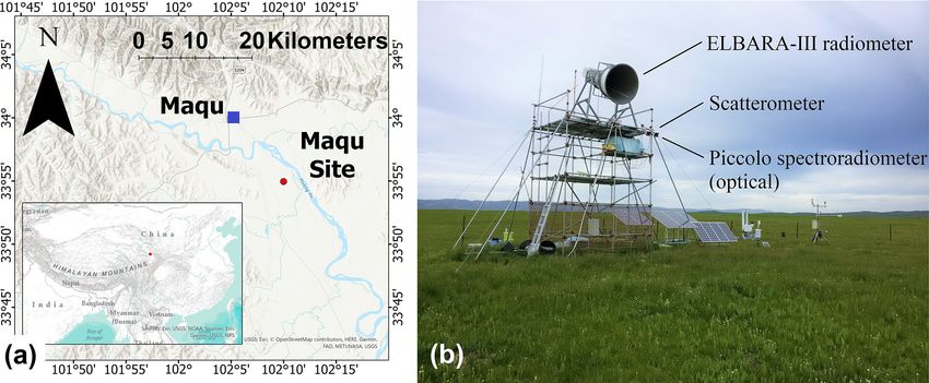
2820                  J. G. Hofste et al.: Year-long, broad-band, microwave backscatter observations of an alpine meadow

       summer periods. Hence further investigation of this scatterometer dataset provides an opportunity to gain new
       insights in hydrometeorological processes, such as freezing and thawing, and how these can be monitored with
       multi-frequency scatterometer observations. The dataset is available via https://doi.org/10.17026/dans-zfb-qegy
                                                                                    0 via the method presented in this
       (Hofste et al., 2021). Software code for processing the data and retrieving σpq
       paper can be found under https://doi.org/10.17026/dans-xyf-fmkk (Hofste, 2021).

1   Introduction                                                   Gamma Remote Sensing AG (Werner et al., 2010), is another
                                                                   scatterometer that operates over 9–18 GHz and measures the
To comprehend the climate of the Tibetan Plateau, also             full polarimetric backscatter autonomously over many eleva-
known as the “Third Pole Environment”, the transfer pro-           tion and azimuth angles. Lin et al. (2016) used it during mul-
cesses of energy and water at the land–atmosphere interface        tiple winter campaigns in the 2009–2012 period at two differ-
must be understood (Seneviratne et al., 2010; Su et al., 2013).    ent locations to study the scattering properties of snow lay-
Main states of interest are the dynamics of soil moisture and      ers. Like in this study, others also designed their scatterome-
temperature (Zheng et al., 2017a). Together with sensors em-       ter architecture around a commercially available vector net-
bedded into the deeper soil layers, microwave remote sensing       work analyser (VNA). For instance, Joseph et al. (2010) used
is suitable to study these dynamics since it directly probes the   data measured by a truck-based system, operating at C- and
top soil layer within the antenna footprint.                       L-band, in summer 2002 to study the influence of corn on
   A ground-based microwave observatory was installed on           the retrieval of soil moisture from microwave backscattering.
an alpine meadow over the Tibetan Plateau, near the town           For every band they placed one antenna to transmit and re-
of Maqu. The observatory consists of a microwave radiome-          ceive on top of a boom. Selection of the individual polariza-
ter system called ELBARA-III (ETH L-Band radiometer for            tion channels was realized using radio-frequency switches.
soil moisture research) (Schwank et al., 2010; Zheng et al.,       Similar is the University of Florida L-band Automated Radar
2017b) and an microwave scatterometer. Both continuously           System (UF-LARS) (Nagarajan et al., 2014), used by for ex-
measure the surface’s microwave signatures with a tempo-           ample Liu et al. (2016), to measure soil moisture at L-band
ral frequency of once every hour. The ELBARA-III was               from a Genie platform during summer 2012. Another exam-
installed in January 2016 and is currently still measuring         ple is the Hongik Polarimetric Scatterometer (HPS) (Hwang
(Zheng et al., 2019; Su et al., 2020); the scatterometer was       et al., 2011), with which microwave backscatter from bean
installed in August 2017 and continued to operate until July       and corn fields was measured in 2010 and 2013 respectively
2019.                                                              (Kweon and Oh, 2015). Similar to our study, Kim et al.
   This paper describes the scatterometer system and the col-      (2014) used a scatterometer with its antenna in a fixed posi-
lected dataset over the period August 2017–August 2018             tion and orientation to measure the backscattering during all
(Hofste et al., 2021). The radar return amplitude and phase        growth stages of winter wheat at L-, C-, and X-band during
were measured over a broad 1–10 GHz frequency band at all          2011–2012.
four linear polarization combinations (vv, hv, vh, hh). The           The temporal resolution and measurement period covered
scatterometer measured the radar return over a prolonged           by the scatterometer dataset reported in this paper permits
period with its antennas in a fixed orientation, resulting in      studying both seasonal and diurnal dynamics of microwave
frequency-dependent incidence angle ranges varying from of         backscattering from an alpine meadow ecosystem. This in
0◦ ≤ θ ≤ 60◦ for L-band (1.625 GHz) to 47◦ ≤ θ ≤ 59◦ for           turn allows for investigating the local soil moisture dynam-
X-band (9.5 GHz). During the summers of 2017 and 2018              ics, the freeze–thaw process, and growth/decay stages of veg-
additional experiments were conducted to assess the angular        etation. Because of the broad frequency range measured (1–
dependence of the backscatter and homogeneity of the local         10 GHz), wavelength-dependent effects of surface roughness
ground surface.                                                    and vegetation scattering can be studied as well.
   Many other studies exist employing ground-based systems            This paper is organized as follows. First the study area is
to study microwave backscatter from land. Rather than an           described. Next, details are provided on the instrumentation
airborne or spaceborne system, ground-based systems allow          used, measurements performed, and method for retrieving
for high temporal coverage and a high degree of control over       the backscattering coefficient σ 0 (m2 m−2 ). We then present
the experimental circumstances. Geldsetzer et al. (2007) and       an overview of the retrieved σ 0 time-series dataset and show
Nandan et al. (2016) used specially developed radar systems        how σ 0 varies across seasons and on a diurnal timescale. In
by ProSensing Inc. to study backscattering from sea ice in the     the discussion section the angular and spatial variability of
period 2004–2011: one system for C-band and another for            σ 0 at the study area and measurement uncertainty are de-
X- and Ku-band. Details on a similar S-band system can be          scribed. Technical details on all aspects of the scatterome-
found in Baldi (2014). The SnowScat system, developed by           ter measurements and σ 0 calculation are included in the Ap-

Earth Syst. Sci. Data, 13, 2819–2856, 2021                                         https://doi.org/10.5194/essd-13-2819-2021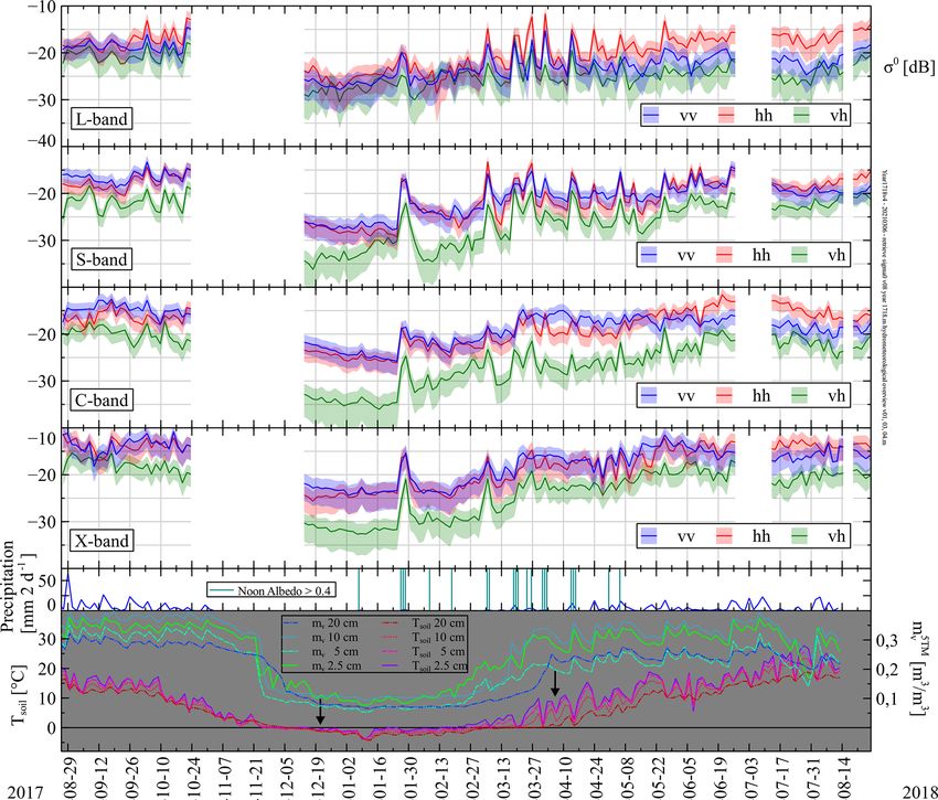
J. G. Hofste et al.: Year-long, broad-band, microwave backscatter observations of an alpine meadow 2821
pendix. A list of symbols can be found at the end of this The depth profile of mv (m3 m−3 ) was measured with an
paper. array of 20 capacitance sensors, type 5TM (manufacturer:
Meter Group), that were installed at depths ranging from
2 Study region and climate 2.5 cm to 1 m (Lv et al., 2018). All sensors in the array are
also equipped with a thermistor, enabling the measurement of
In August 2017 the scatterometer was installed on the tower Tsoil (◦ C). The soil moisture and temperature was logged ev-
of the Maqu measurement site (Maqu site) (Zheng et al., ery 15 min for the period of August 2017–August 2018 with
2017b) and operated over the period August 2017–June Em50 data loggers (manufacturer: Meter Group) that were
2019. The Maqu site is situated in an alpine meadow ecosys- buried near the sensors. The location of the buried sensor
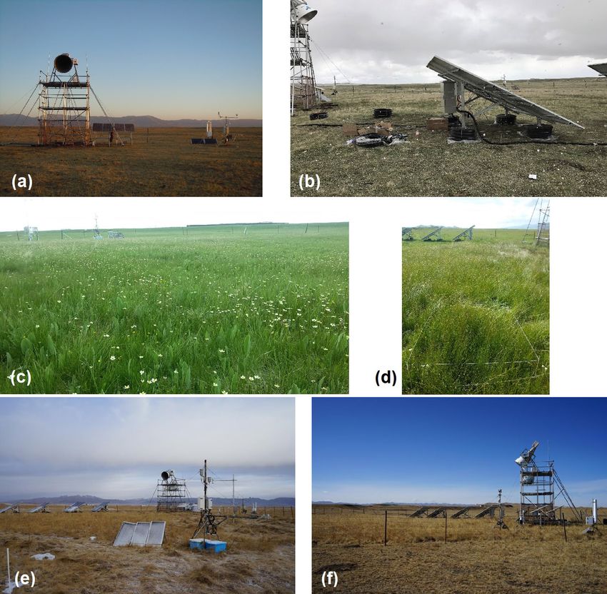
tem (Miller, 2005) on the Tibetan Plateau, Fig. 1a. The site’s array is indicated in Fig. 2. Results of these hydrometeoro-
coordinates are 33◦ 550 N, 102◦ 100 E, at 3500 m elevation. logical measurements over the period August 2017–August
The site is located close to the town Maqu of the Gansu 2018 can be found in Appendix Sect. A2 as well. With a
province of China. handheld impedance probe, type ThetaProbe ML2x (manu-
Besides the scatterometer, other remote sensing sen- facturer: Delta-T Devices), the spatial variability of mv in
sors placed on the tower are the ELBARA-III radiometer the top 2.5–5 cm soil layer over the Maqu site was measured
(Schwank et al., 2010) and the optical spectroradiometer sys- (Appendix Sect. A3).
tem Piccolo (MacArthur et al., 2014), Fig.1b. The ELBARA- To quantify the vegetation cover at the Maqu site, mea-
III system has been measuring L-band microwave emission surements were performed on 2 d during the 2018 summer,
since January 2016 to this date (Zheng et al., 2019; Su et al., namely 12 July and 17 August. Vegetation height, above-
2020). The Piccolo system measured the reflectance and sun- ground biomass (fresh and oven-dried), and leaf area in-
induced chlorophyll fluorescence of the vegetation over the dex (LAI) (m2 m−2 ) were measured at ten 1.2 × 1.2 m2 sites
period July–November 2018. around the periphery of the “no-step zone” indicated in
According to Peel et al. (2007) the climate at Maqu is char- Fig. 2. The vegetation height of a single site was determined
acterized by the Köppen–Geiger classification as “Dwb”: as the maximum value of the histogram obtained by taking
cold with dry winters. Winter (December–February) and ≥ 30 readings with a thin ruler at random points within the
spring (March–May) are cold and dry, while the summer site area. For each site, above-ground biomass and LAI were
(June–August) and autumn (August–November) are mild determined from harvested vegetation within one or two disk
with monsoon rain. areas defined by a 45 cm diameter ring. Immediately after
The ecosystem classification of the Maqu site is “alpine harvest all biomass was placed in airtight bags so that the
meadow” according to Miller (2005). The vegetation around fresh and dry biomass could be determined by weighing the
the Maqu site consists of grasses for the most part. The grow- bag’s content before and after drying in an oven. The LAI
ing season starts at the end of April and ends in October, was determined immediately after harvest with part of the
when above-ground biomass turns brown and loses its water. harvested fresh biomass by the method described in He et al.
During the growing season the meadows are regularly grazed (2007). The obtained average quantities over the 10 sites are
by livestock. To prevent the livestock from entering the site summarized in Appendix Sect. A4.
and damaging the equipment, a fence is placed around the
Maqu site. As a result there is no grazing within the site,
3.2 Scatterometer
causing the vegetation to be more dense and higher than
that of the surroundings. Also a layer of dead plant mate- 3.2.1 Instrumentation
rial from the previous year remains present below the newly
emerged vegetation. In Appendix Sect. A1 some photographs The main components of the scatterometer are a two-port
are shown of the Maqu site during different seasons, which vector network analyser (VNA), type PNA-L 5232A (man-
provide an impression of the site’s phenology. ufacturer: Keysight); four 3 m long phase-stable coax ca-
bles, type Sucoflex SF104PEA (manufacturer: Huber + Suh-
ner); and two dual-polarized broad-band horn antennas, type
3 Methodology
BBHX9120LF (manufacturer: Schwarzbeck); see Fig. B1.
3.1 Supporting measurements The antenna radiation patterns are measured in the prin-
cipal planes by the manufacturer over the 1–10 GHz band
Together with the scatterometer, measurements following hy- (Schwarzbeck Mess-Elektronic OHG, 2017). As a sum-
drometeorological quantities were recorded over the period mary, the full width at half maximum (FWHM) intensity
August 2017–August 2018: depth profile of volumetric soil beamwidths over frequency are shown in Fig. B3. To pro-
moisture mv (m3 m−3 ) and soil temperature Tsoil (◦ C), air tect the VNA from weather it is placed inside a waterproof
temperature Tair (◦ C), precipitation (mm), and the short- and enclosure equipped with fans to provide air ventilation.
long-wave up- and downward irradiance (W m−2 ). Details on Deployed reference targets to calibrate the scatterometer
used sensors can be found in Appendix Sect. A2. were a rectangular plate and two dihedral reflectors. The
https://doi.org/10.5194/essd-13-2819-2021 Earth Syst. Sci. Data, 13, 2819–2856, 2021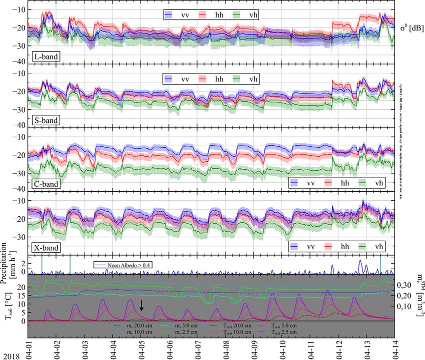
2822                   J. G. Hofste et al.: Year-long, broad-band, microwave backscatter observations of an alpine meadow

Figure 1. (a) Location of Maqu measurement site on eastern part of the Tibetan Plateau. (b) Tower of Maqu site containing the scatterometer,
the ELBARA-III radiometer, and Piccolo optical spectroradiometer.

Figure 2. Map of the Maqu site. Scatterometer footprints for C-band with vv polarization are shown for different α0 (40, 55, 70◦ ) and φ
(−30, −20, . . ., 30◦ ) angles. For time-series measurement antennas were fixed at α 0 = 55◦ and φ = 0◦ .

rectangular plate reflector was constructed from lightweight            tion from this mast, it was covered by pyramidal absorbers,
foam board covered with 100 µm aluminium foil and had                   type 3640-300 (manufacturer: Holland Shielding), having a
frontal dimensions a = 85 cm × b = 65 cm. A small dihe-                 35 dB reflection loss for normal incidence at 1 GHz.
dral reflector was constructed from steel, and its frontal
dimensions were a = 57 cm × b = 38 cm. A second large
dihedral reflector was also constructed with foam board                 3.2.2    Experimental setup and procedures
and aluminium foil, and its frontal dimensions were a =
                                                                        The scatterometer is placed on a tower as shown in Fig. 1b.
120 cm × b = 65 cm. A height-adjustable metal mast was
                                                                        The two antenna apertures are at a distance approximately
used to position the reference targets. To minimize reflec-
                                                                        Hant = 5 m above the ground (Hant depends on the an-

Earth Syst. Sci. Data, 13, 2819–2856, 2021                                                https://doi.org/10.5194/essd-13-2819-2021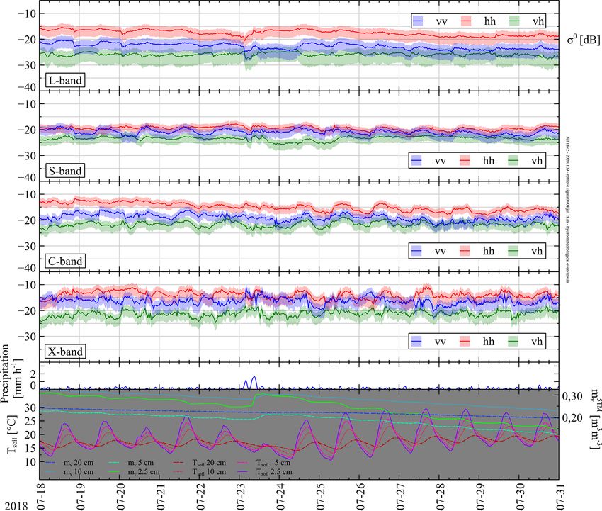
J. G. Hofste et al.: Year-long, broad-band, microwave backscatter observations of an alpine meadow                            2823

tenna boresight angle α0 ) and are separated from each other      3.2.3   σ 0 retrieval procedure
horizontally by Want = 0.4 m. The connection scheme of
                                                                  The power received by a monostatic radar or scatterometer
the VNA and the two antennas is described in Appendix
                                                                  system from a distributed target with backscattering coeffi-
Sect. B1. In Appendix Sect. B2 further details on the setup                0 (θ ) (m2 m−2 ) is given by the radar equation (Ulaby
                                                                  cient σpq
geometries can be found. During all experiments, VNA mea-
                                                                  et al., 1982)
surements were performed with a stepped 0.75–10.25 GHz
frequency sweep at 3 MHz resolution (3201 points). The                       λ2
                                                                                           Z 2
                                                                                              G 0
dwell time per measured frequency was 1 µs, which is equiv-       PpRX =           P TX 2
                                                                                     q G          σ (θ) · dA,                  (1)
                                                                            64π  3       0
                                                                                              R 4 pq
alent to a two-way travelling distance for the microwave
signal of 150 m. The intermediate-frequency (IF) bandwidth        where it is assumed that the same antenna is used for both
was minimized to 1 KHz to increase the signal-to-noise ratio.     transmitting (TX) and receiving (RX). PqTX is the transmitted
   The radar return from the rectangular metal plate refer-       and PpRX the received power respectively (W). The subscripts
ence target was used to calibrate the scatterometer for the co-   of the powers refer to the linear polarization directions: hor-
                                                                  izontal (h) or vertical (v). With σpq 0 the first subscript refers
polarization channels. The two metal dihedral reflectors were
used as depolarizing reference targets (Nesti and Hohmann,        to the polarization direction of the scattered and the second
1990) to calibrate the cross-polarization channels. We used       to that of the incident wave. G (–) denotes the normalized
two dihedrals, measured at different distances R0 (m), in or-     angular gain pattern of the antenna with peak value G0 (–).
der to meet requirements concerning target size, target dis-      Equation (1) represents an ideal lossless system – in practice
tance (plane wave criteria), and ground-to-target interference    any scatterometer has frequency-dependent losses or other
removal. Readers are referred to Appendix Sect. B3 for the        signal distortions. These frequency-dependent phase and am-
measurement details and validation-exercise results.              plitude modulations can be accounted for by measuring the
   Time-domain filtering, or gating, was used as part of post-    radar return of a reference target Pp0 with known radar cross
processing to remove the antenna-to-antenna coupling and          section (RCS) σpq (m2 ) (Eq. B2) to calibrate the system. This
undesired scattering contributions from the radar return sig-     procedure, often referred to as external calibration, is mathe-
nal for both the reference target and the ground return mea-      matically represented by
surements. The application of gating with VNA-based scat-
                                                                                    4 Z G2
terometers is described in more detail in for example Jersak        RX      0 (R0 )
                                                                  Pp = Pp                   σ 0 (θ ) · dA,                       (2)
et al. (1992) or De Porrata-Dória i Yagüe et al. (1998). De-                   σpq      R 4 pq
tails on our gating process and related peculiarities regarding
                                                                  where R0 (m) is the distance at which the reference target
our scatterometer can be found in Appendix Sect. B4.
                                                                  was measured. In the case of a scatterometer with narrow
   In this paper, we focus on the time-series measurements
                                                                  beamwidth antenna, all integrand terms of Eq. (2) can be ap-
of σ 0 over a 1-year period, during which measurements were
                                                                  proximated as being constants, the so-called “narrow-beam
taken either once or twice per hour. With this experiment,
                                                                  approximation” (Wang and Gogineni, 1991), so that we ob-
the antennas were fixed on a tower rod, such that the angle
                                                                  tain
between the antenna boresight line and the ground surface
normal α0 was 55◦ and the azimuth angle φ was fixed at 0◦                      (R0 )4 1
as shown in Fig. 2. Although varying the antennae orienta-        PpRX = Ppc               σ 0 (θ)Afp ,                         (3)
                                                                                σpq (Rfp )4 pq
tions (using automatic motorized rotational stages) to mea-
sure backscatter under various incidence and azimuth angles       where Afp is the scatterometers “footprint”, notably the area
would be preferable from an experimental perspective, this        (m2 ) for which the surface projected antenna beam intensity
approach was abandoned because it would make the setup            is equal to or larger than half its maximum value. Rfp (m)
extra vulnerable to system failures. Measurements of σ 0 for      refers to the distance between the antenna and footprint cen-
different α0 and φ angles at the Maqu site were, however,         tre.
                                                                     For this dataset σpq0 (θ ) is estimated by employing Eq. (3)
performed during 3 separate days. These measurements are
discussed in Sect. 5.3. Before installing the scatterometer       in combination with a mapping of the term G2 /R 4 (x, y) from
at the Maqu site, exploratory experiments were performed          Eq. (2) over the ground surface. Due to the wide antenna radi-
in which σ 0 over α0 was measured for asphalt and subse-          ation patterns, especially with low frequencies, the area that
quently compared to results in other studies (Sect. 5.1). Ta-     is to be associated with the measured scatterometer signal,
ble 1 summarizes all experiment geometries and dates of           i.e. the footprint, is typically not located where the antenna
execution. For the angular-variation experiments the scat-        boresight line intersects the ground surface. Instead the foot-
terometer antennas were mounted on a motorized rotational         print appears closer to the tower base. Figure 3 demonstrates
stage. Depending on the angle α0 , Hant would vary accord-        this effect for the case of 5 GHz at α0 = 55◦ , by showing the
ing to Hant = H0 − 0.5 cos(α0 ), with H0 = 2.95 or 5.2 m for      mapping of G2 /R 4 over the ground surface. This footprint-
the asphalt or Maqu experiments respectively. All angular-        shift effect is strongest with the widest antenna radiation pat-
variation experiments were conducted within one afternoon.        terns (thus with low frequencies) and for large α0 angles. The

https://doi.org/10.5194/essd-13-2819-2021                                         Earth Syst. Sci. Data, 13, 2819–2856, 2021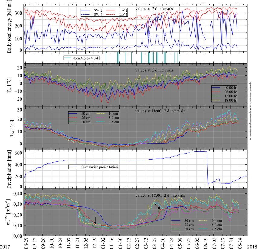
2824                   J. G. Hofste et al.: Year-long, broad-band, microwave backscatter observations of an alpine meadow

Table 1. Overview of performed scatterometer experiments and their respective α0 and φ ranges. Antennae aperture height Hant depends on
α0 .

                                       Date                  φ (◦ )                           α0 (◦ )             Hant (m)
       Angular variation σ0 asphalt    4 May 2017            00                               35, 40, . . ., 75   2.55, 2.55, . . ., 2.80
       Angular variation σ0 Maqu       25 August 2017        −20, −15, −10, −05, 00, +10,     35, 40, . . ., 70   4.80, 4.80, . . ., 5.05
                                                             +15, +20
       Angular variation σ0 Maqu       29 June 2018          −30, −20, −15, −10, −05, 00,     35, 40, . . ., 70   4.80, 4.80, . . ., 5.05
                                                             +05, +10, +20, +25, +30
       Angular variation σ0 Maqu       19 August 2018        −30, −20, −10, 00, +10, +20,     35, 55, 70          4.80, 4.90, 5.05
                                                             +30,
       Time series σ0 Maqu             26 August 2017–       00                               55                  4.70
                                       26 August 2018

                                                                            (1988)1 . This quantity is measured over the full 0.75–
                                                                            10.25 GHz band at angle α0 : Ee (f, α0 ). Bandwidths
                                                                            (BW) are selected based on the change in G(α, β) over
                                                                            frequency (Appendix Sect. B4), the number of indepen-
                                                                            dent frequency samples N that may be retrieved from
                                                                            BW, and the estimated change in backscattering proper-
                                                                            ties over frequency of the ground surface as is discussed
                                                                            in Appendix Sect. C2. Result is the bandwidth selection
                                                                            Ee (BW, α0 ).

                                                                         2. With BW and α0 as input, G2 /R 4 (x, y) is mapped for
Figure 3. Example of G2 /R 4 (x, y) with Gaussian antenna radia-            all frequencies within BW using the antenna radiation
tion patterns. Plot normalized to its peak value. x and y are ground        patterns measured by the manufacturer. The region as-
surface coordinates. The white triangle at coordinate (0,0) repre-          sociated with 50 % of the total projected intensity onto
sents the tower location and the other white triangle indicates the         the ground is determined to set appropriate gating times,
intersection point of the antenna boresight line and the ground sur-        or distances rsg and reg (m), and for calculating the Afp ,
face. α0 = 55◦ , f = 5 GHz and polarization is vv.                          Rfp , and the θ range. Half the pulse width c/(2BW) is
                                                                            subtracted from rsg and added to reg , and quantities Afp ,
                                                                            Rfp , and the θ range are changed accordingly.
footprint position and dimensions were found using the map-
ping G2 /R 4 (x, y) over the ground surface. The applied cri-            3. The gate is applied to Ee (BW, α0 ), resulting in the gated
terion was that the footprint contains 50 % of the total pro-                                     g
                                                                            backscattered field Ee (BW, α0 ), where the superscript g
jected intensity onto the ground surface. After the footprint               indicates that the signal is gated.
edges were defined the incidence angle ranges were derived
                                                                                                                                            g
from them using trigonometry.                                            4. The bandwidth-average coupling remnant hEcr i
   Because of the low directivity (gain) of the antennas and                (V m−1 ) and minimal detectable signal Eb (V m−1 )
                        0 over θ , there is an inherent uncer-                                       g
unknown nature of σpq                                                       are subtracted from Ee (BW, α0 ) for each measured
                         0 values (for a certain θ range). This                            g
tainty in our retrieved σpq                                                 frequency. Ecr is an offset formed by part of the signal
matter is discussed further in Sect. 5.2.                                   transmitted from the transmit antenna coupling directly
   In Fig. 4 the procedure for deriving the backscattering co-              into the receive antenna (antenna cross coupling).
efficient is depicted. The equations used therein are derived               Although the majority of this coupling can be filtered
from Eq. (3). Refer to Appendix Sect. C1 for more informa-                  out by using time-domain gate filtering, a remnant is
tion. The different steps indicated in the figure are explained             still present (hence “coupling remnant” in the subscript)
here.                                                                       and must be accounted for (Appendix Sect. E4). Note
                                                                                                         g
                                                                            that the same gate as with Ee is applied. A similar form
  1. We start with Ee (V m−1 ), the measured backscattered
     electric field from the ground target incident on the re-             1 In reality the measured fields or signals remain complex until
     ceiving antenna. The subscript e denotes “envelope”               after the gating process. We, however, stick to this terminology for
     magnitude of the complex signal, as in Ulaby et al.               clarity.

Earth Syst. Sci. Data, 13, 2819–2856, 2021                                              https://doi.org/10.5194/essd-13-2819-2021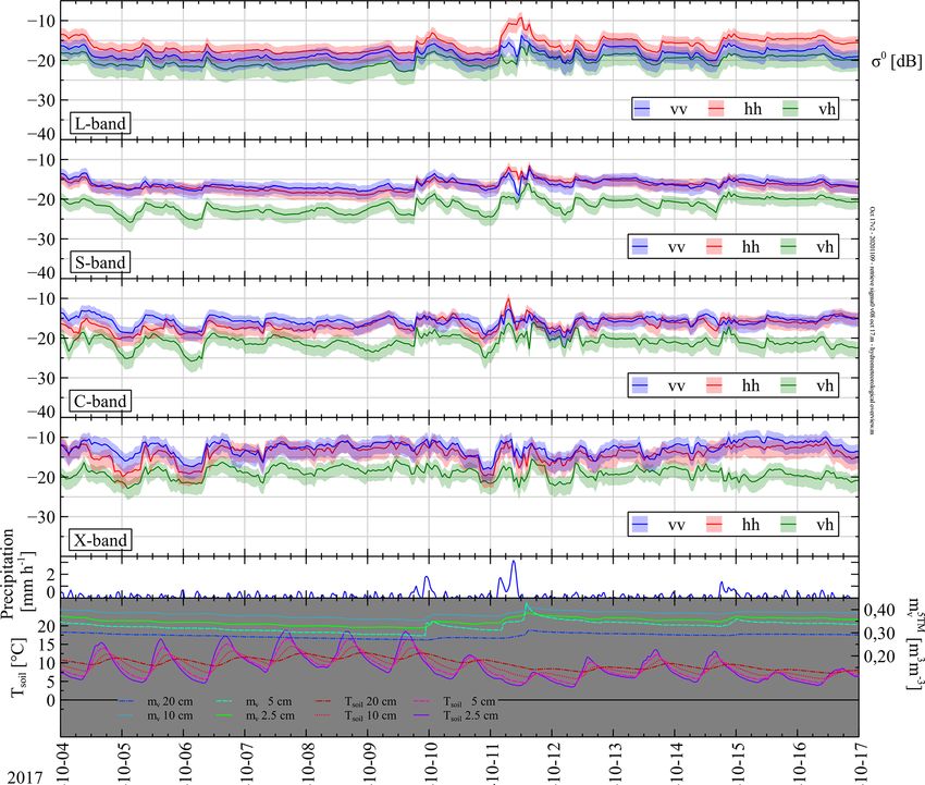
J. G. Hofste et al.: Year-long, broad-band, microwave backscatter observations of an alpine meadow                                      2825

Figure 4. Flow chart of σ 0 derivation process. Inputs are the measured backscattered electric fields of the surface target Ee (f, α0 ) and the
calibration standard E0 (f ). The process follows from 1 to 11 in sequence.

                                      g
     of offset subtraction from Ee was done in for example                    9. The measured response from the mast without refer-
                                                                                               g0
     Nagarajan et al. (2014). Next, the result is squared and                    ence target Eb0 (BW) (V m−1 ) is subtracted from the
     converted into intensity I (BW, α0 ) (W m−2 ).                              reference target response. Subscript b0 denotes back-
                                                                                 ground calibration, and the superscript g0 indicates that
  5. To reduce the radiometric uncertainty due to fading we                      the same gate was used as with the reference target re-
     perform frequency averaging. The number of statisti-                        sponse. Also Eb is subtracted here. The result is squared
     cally independent frequency samples N within BW is                          and converted into intensity I0 (BW) (W m−2 ).
     calculated with 1R = reg − rsg (m). Please refer to Ap-
     pendix Sect. C2 for more information.                                 10. The I0 (BW) is used to calculate the factor K (W m−2 ),
                                                                               given the footprint area Afp and centre distance Rfp
  6. From the I (BW, α0 ) spectrum N intensities are selected
                                                                               (Eq. C2).
     at equidistant intervals of 1f = BW/N − 1 (Hz) and
     averaged to IN (α0 ).                                                 11. The final step is the application of Eq. (C1) with I (α0 )
  7. With IN (α0 ) and N, the average received intensity I (α0 )               and K(α0 ) as inputs to obtain σ 0 . By steps 2 and 6 the
     (W m−2                                                                    derived σ 0 is to be associated with the chosen BW and
           √) is calculated using Eq. (C4). The denominator                    calculated θ range. By step 7 a 68 % confidence interval
     1 ± 1/ N implies that I is estimated with a 68 % con-
     fidence interval.                                                         applies to σ 0 .

  8. The gated backscattered signal from the reference target             4    Measurement results
       g0
     E0 (BW) (V m−1 ) (subscript 0 represents “reference”;
     superscript g0 stands for “gate” during reference mea-               For the analyses in this paper we discuss results of four band-
     surements) is determined for the full 0.75–10.25 GHz                 widths BW, picked amidst frequency ranges typically used in
     band under the assumption that G ≈ 1 for all frequen-                microwave remote sensing: 9–10 GHz (X-band), 4.5–5 GHz
     cies (see Appendix Sect. B4). After gating the relevant              (C-band), 2.5–3 GHz (S-band), and 1.5–1.75 GHz (L-band).
               g0
     BW of E0 is selected.                                                The widths decrease with wavelength due to the expected

https://doi.org/10.5194/essd-13-2819-2021                                                  Earth Syst. Sci. Data, 13, 2819–2856, 2021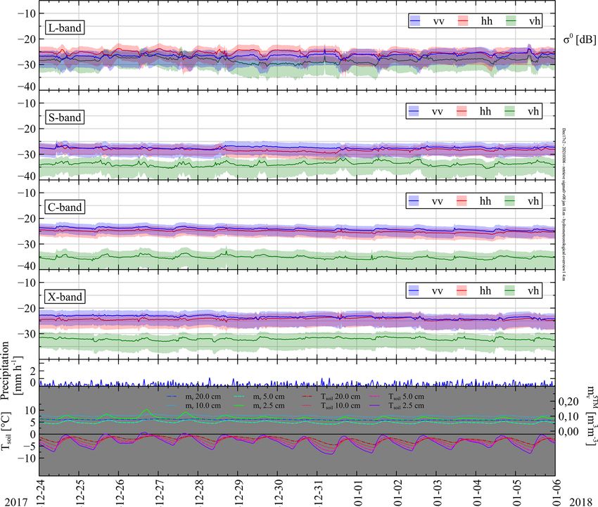
2826                  J. G. Hofste et al.: Year-long, broad-band, microwave backscatter observations of an alpine meadow

frequency resolution of the target’s scattering response (Ap-       This behaviour was also observed by Oh et al. (1992), albeit
pendix Sect. C2) and the antenna-radiation-pattern change           for bare soil. We, however, may compare our situation to that
over frequency (Appendix Sect. B4). Presented in this sec-          of bare soil during winter, when there is no fresh biomass.
tion is, first, a global overview of the retrieved σpq0 over the    When vegetation was present, σhh   0 was stronger for all bands,

period 26 August 2017–26 August 2018, followed by a 13 d            as is visible during June–August 2018. This was however
time series of σpq 0 at the highest temporal resolution during      not the case during August–September 2017, when the veg-
the thawing period in April 2018.                                   etation probably still contained water. Somewhat stronger
   Figure 5 presents an overview of the time-series data of         backscatter, 0.5–1 dB, for hh than for vv polarization was
  0 over the whole August 2017–2018 period for all consid-
σpq                                                                 also reported for grassland in Ulaby and Dobson (1989) with
ered bandwidths in L-, S-, C-, and X-band, along with Mv            40 ≤ θ ≤ 60◦ for S- and X-band. For C-band they reported
and Tsoil at four depths ranging from 2.5 to 20 cm and pre-         no clear difference. Yet another study, (Kim et al., 2014),
cipitation. Based on observed albedo values, days at which          measured 3–4 dB higher backscatter for hh than for vv po-
a layer of snow was present are indicated. For visibility rea-      larization when measuring wheat at L-band (θ = 40◦ ). Our
sons the graphs only display measurements taken at 18:10 LT         results for L-band were similar. Cross-polarization σ 0 levels
with 2 d intervals and one cross-polarization channel (σvh 0 and    were, as expected, lower than those of co-polarization. Dur-
  0
σhv are within each other’s confidence intervals). Data of the      ing the winter period this difference was largest, especially
radar return and σpq  0 for November 2017 are not available,        with C-band. For L-band, on the other hand, this difference
while those of late June–Early July 2018 will become avail-         in σ 0 levels between co-polarization and cross polarization
able at a later stage.                                              was quite small.
   We observe for all bands and polarizations that σ 0 is high-        Next, four 13 d time series of σ 0 at 30 min intervals are
est in summer and autumn, while it is lowest during win-            presented. When selecting these periods we tried avoid-
ter. The same observations were made with satellites over           ing strong precipitation events as much as possible, since
the Maqu area for L-band (Wang et al., 2016) and C-band             these complicate the interpretation. In Appendix Sect. D
(Dente et al., 2014). This behaviour can be explained by the        time series during October 2017 (Fig. D1), December 2017
fact that in summer and autumn Mv and the amount of fresh           (Fig. D2), and July 2018 (Fig. D3) can be found. Here we
biomass is highest. As a result, the high dielectric constant       shall describe the retrieved σpq0 during a 13 d period in April

of moist soil in combination with the rough surface and pres-       2018 (Fig. 6) when the thawing process was ongoing.
ence of water in the vegetation results in strong backscatter-         The most prominent features in Fig. 6 are the diurnal vari-
ing. During winter, however, there is little liquid water, i.e.                 0 that are clearly caused by changes in M . For
                                                                    ations of σpq                                              v
Mv , present in the soil and no fresh biomass (dry biomass          S-, C-, and X-bands we observe that σ 0 increases during day-
however remains present; see Fig. A1). Black arrows indicate        time due to the increase in liquid water in the top soil due to
frozen and thawed soil at 25 cm depth (Appendix Sect. A2).          thawing, and at night σ 0 drops as most of the water freezes
The dielectric constant of the soil therefore is lower com-         again. For L-band this behaviour is also visible, though not as
pared to that of moist soil, and there is little to no scattering   pronounced. The Mv changes at different depths are consis-
from the dried out vegetation, resulting in a lower σpq   0 . All
                                                                    tent with this difference: the strongest diurnal variation in liq-
aforementioned effects are described in, for example, (Ulaby        uid water was measured by the probes at 2.5 and 5 cm depth,
and Long, 2017). There were, however, also peaks of σpq        0
                                                                    while those at 10 and 20 cm do not change as much. On some
during winter, for example on 26 January, which coincided           days, for example on 4 and 5 April, or on 10 April, we ob-
with snowfall. In (Lin et al., 2016) strong backscatter incre-      serve diurnal changes in σ 0 (most pronounced for X-band),
ments due to fresh snowfall were also observed for X-band.          while the Mv measured by the 5TM sensors at 2.5 and 5 cm
Apparently, this behaviour is similar with the longer wave-         depth showed little variation. This may suggest that the freez-
lengths as the graphs show.                                         ing and thawing during those days occurred only in the very
   When comparing the four bands we observe that, in gen-           top soil layer, just below the air–soil interface where it was
eral, the backscattering is highest for X-band and lowest for       outside the influence zone of the 5TM sensors. The time lag
L-band or S-band. This difference is mainly driven by the           between the drop of σ 0 (first) and the drop of 5TM Mv (sec-
wavelength-dependent response to the surface roughness of           ond) is caused by the same phenomena as the freezing starts
the soil and vegetation during the summer and autumn pe-            at the top soil layer and progresses downward. The time lag
riod. For longer wavelengths the soil surface roughness ap-         during thawing was smaller. In general the magnitude of the
pears smoother than for the shorter wavelengths, resulting in       σ 0 change was largest for X-band and smallest for L-band,
stronger specular reflection, thus lower backscatter. A similar     though exceptions exist. See for example 3 April, where for
argument holds for the vegetation: its constituents are small       L-band σhh0 drops almost 10 dB, which is more than for other
compared to the longer wavelengths; thus little volume scat-        bands. At the same time Mv at 20 cm depth also shows strong
tering occurs.                                                      variation, while Mv at 10 cm changes less.
   Except for during the summer, backscatter for vv polar-
ization was equal to or higher than that for hh polarization.

Earth Syst. Sci. Data, 13, 2819–2856, 2021                                           https://doi.org/10.5194/essd-13-2819-2021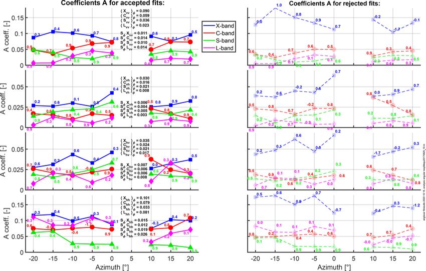
J. G. Hofste et al.: Year-long, broad-band, microwave backscatter observations of an alpine meadow                                    2827

                                       0 (m2 m−2 ) for L-, S-, C-, and X-band, M , and T
Figure 5. Time-series measurements of σpq                                       v        soil from August 2017 to 2018. Shown are
measurements taken at 18:10 LT with 2 d intervals. Shaded regions indicate 66 % confidence intervals for σpq0 . The antenna boresight angle
was fixed at α0 = 55 . The incidence angle ranges were band and polarization dependent. The widest ranges were 0◦ ≤ θ ≤ 60◦ for L-
                       ◦
band, 20◦ ≤ θ ≤ 60◦ for S-band, 36◦ ≤ θ ≤ 60◦ for C-band, and 47◦ ≤ θ ≤ 59◦ for X-band. Bottom graphs show measured precipitation per
2 d (snowfall identified by noon albedo), volumetric soil moisture m5TM
                                                                      v    (m3 m−3 ), and soil temperature Tsoil at indicated depths. Arrows
indicate frozen/thawed soil at 25 cm. Spatial average volumetric soil moisture Mv is estimated as Mv = m5TM
                                                                                                          v    ± 0.04 m3 m−3 .

5     Discussion                                                        5.2    Measurement uncertainty

5.1    Reference measurements for asphalt                               In the derivation of σ 0 we distinguish four sources of uncer-
                                                                        tainty: (i) fading (Sect. 3.2.3), (ii) the temperature-induced
In order to check our scatterometer setup and σ 0 re-                   radar return uncertainty 1ET (V m−1 ), (iii) reference target
trieval procedure an experiment was performed in which the              measurement uncertainty 1K (in dB, as it is a relative value),
backscatter of asphalt was measured and subsequently com-               and (iv) the low-directivity-induced uncertainty.
pared to results found in other studies. This exercise is de-              First we describe (ii) and (iii), which are systematic
scribed in Appendix Sect. F. We found that our results for              sources of uncertainty. In this context we also consider the
X-band with co-polarization and S-band for vv and vh po-                system’s offsets levels formed by the antenna-to-antenna
                                                                                               g
larization match with those reported in Ulaby and Dobson                coupling remnant Ecr (V m−1 ) and the minimum signal
(1989) and Baldi (2014) respectively. For L-band a proper               strength measurable by the VNA, or background Eb (V m−1 ).
comparison was not possible due to the width of our antenna             The former is derived from measurements with the antennas
patterns. We could not find other studies reporting backscat-           aimed skywards. From Eb the minimum measurable RCS
ter for C-band to compare our results to.                               (given a certain distance R to target) σmin can be calculated

https://doi.org/10.5194/essd-13-2819-2021                                                Earth Syst. Sci. Data, 13, 2819–2856, 2021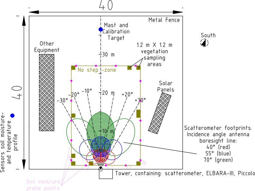
2828                  J. G. Hofste et al.: Year-long, broad-band, microwave backscatter observations of an alpine meadow

                                       0 (m2 m−2 ) for L-, S-, C-, and X-band, precipitation, M , and T
Figure 6. Time-series measurements of σpq                                                      v       soil during 13 d in April 2018.
                                                       0 . The antenna boresight angle was fixed at α = 55◦ . The incidence angle ranges
Shaded regions indicate 66 % confidence intervals for σpq                                            0
were band and polarization dependent. The widest ranges were 0◦ ≤ θ ≤ 60◦ for L-band, 20◦ ≤ θ ≤ 60◦ for S-band, 36◦ ≤ θ ≤ 60◦ for C-
band, and 47◦ ≤ θ ≤ 59◦ for X-band. Bottom graphs show measured precipitation (mm h−1 ) (snowfall identified by noon albedo), volumetric
soil moisture m5TM
                v    (m3 m−3 ), and soil temperature Tsoil at indicated depths. Arrow indicates thawing of soil at 25 cm. Spatial average
volumetric soil moisture content Mv is estimated as Mv = m5TM
                                                            v    ± 0.04 m3 m−3 .

via Eq. (3), where instead of the product σ 0 Afp a RCS value          1IN (W m−2 ) is a statistical error that follows from 1ET ,
is to be calculated using the power levels associated with Eb .        1K is converted from a maximum possible error into a sta-
Appendix Sect. E contains detailed information on all con-             tistical error√with a (2/3) probability confidence interval, and
sidered systematic sources of uncertainty and offsets, starting        the term 1/ N represents a statistical error caused by fad-
with an overview (Appendix Sect. E1), followed by sections             ing. In the right term the three uncertainty contributions are
on 1ET (Appendix Sect. E2), 1K (Appendix Sect. E3), and                merged into one statistical uncertainty 1σ 0 (m2 m−2 ), which
  g
Ecr (f ) (Appendix Sect. E4).                                          is a 66 % confidence interval for σ0 . In this paper these 66 %
   Starting with Eq. (C1) it can be shown (see Appendix                confidence intervals are presented in all figures showing our
Sect. E5) that the three estimated types of uncertainty,               retrieved σ 0 . To give an indication of the magnitude of 1σ 0 ,
namely fading, temperature-induced radar return uncertainty            some typical values over band, polarization, and season are
(1ET ), and reference target measurement uncertainty (1K),             summarized in Table 2. Presented values were retrieved from
can be combined in a model for total σ 0 uncertainty:                  the calculated time-series results of Sect. 4.
                                                                           The low-directivity-induced uncertainty (iv) is not quan-
               IN ± 1IN       IN
σ0 =                 √  =    ± 1σ 0 .                     (4)      tifiable in the sense that with the time-series experiments
             2
         K ± 3 1K 1 ± 1/ N    K                                        backscatter was not repeatedly measured at different α0 an-

Earth Syst. Sci. Data, 13, 2819–2856, 2021                                              https://doi.org/10.5194/essd-13-2819-2021
J. G. Hofste et al.: Year-long, broad-band, microwave backscatter observations of an alpine meadow 2829
Table 2. Example uncertainty values 1σ 0 (dB) per bandwidth, po- vegetation canopy, and, second, we present it to assess the
larization, and overall σ 0 level. spatial homogeneity of σ 0 (θ ) over the Maqu site surface by
also measuring backscatter at different azimuth angles (φ).
L-band S-band C-band X-band As explained in Appendix Sect. C2, the single footprint area
High σ 0 levels (typical in summer) for the σ 0 time-series measurements should be representa-
tive for the whole Maqu site surface. Due to practical limita-
vv +1.6 to −2.5 +1.3 to −1.9 +1.4 to −2.1 +1.7 to −3.0
tions of possible φ angles and because of the wide antenna
vh +1.7 to −3.0 +1.3 to −1.9 +1.4 to −2.2 +1.6 to −2.7
hv +1.8 to −3.2 +1.3 to −1.9 +1.4 to −2.0 +1.6 to −2.7 beamwidths, the footprints of used α0 and φ combinations in
hh +1.6 to −2.5 +1.2 to −1.7 +1.3 to −2.0 +1.7 to −2.9 this experiment overlap partially, as is shown in Fig. 2. How-
ever, since we employ frequency averaging to reduce the fad-
Low σ 0 levels (typical in winter)
ing uncertainty for every footprint, we argue that the σ 0 val-
vv +2.3 to −5.2 +1.9 to −3.7 +1.7 to −2.9 +2.1 to −4.2 ues retrieved per (overlapping) footprint may nevertheless be
vh +2.3 to −5.2 +2.4 to −5.9 +2.6 to −8.3 +2.3 to −5.2 compared to each other for this section’s analysis.
hv +2.4 to −6.0 +2.5 to −6.6 +2.5 to −6.4 +2.0 to −4.9
hh +2.3 to −5.3 +1.7 to −2.8 +1.7 to −2.7 +1.9 to −3.8
As a means to quantitatively evaluate the σ 0 behaviour
with respect to the θ and φ angle, the data are grouped in sets
of σ 0 over α0 for every angle φ, BW, and polarization. In
Appendix Sect. G, Fig. G1 examples of such sets are shown.
gles. With such measurements, sets of PqRX (α0 ) would be ob- Next, an iterative least-squares non-linear fitting algorithm is
tained that can be deconvolved into σ 0 (θ ), since G(α, β) is applied to fit each set to the model:
known (see Eq. 2). This deconvolution approach was per-
formed by, for example, Axline (1974) and Ulaby et al. σ 0 = A cos(θ )B , (5)
(1983). It is possible, however, to give an estimate of the low-
directivity-induced uncertainty, inherent to our σ 0 retrieval where A is a constant (m2 m−2 ) and B is either 1 for an
method, with a simple numerical experiment in which the isotropic scatterer or 2 for a surface in accordance with Lam-
scatterometer radar return is simulated (Eq. 2) using a pre- bert’s law (Clapp, 1946). For each α0 we find the coordinate
defined function for σ 0 (θ ). We may use for example the em- for which G2 /R 4 is maximum and use that position’s angle
pirical model of σpq 0 (θ) for grassland developed in Ulaby and
of incidence θ together with the centre σ 0 value of the 66 %
Dobson (1989) with measurement data from several other confidence interval for the fitting process. As a next step, we
studies. Applying the method of Sect. 3.2.3 on the simu- reduced the number of fitting possibilities by selecting for
lated radar return, we obtain for 4.75 GHz at vv polarization each polarization–BW combination the most likely value for
0 = −14.4 dB for 34◦ ≤ θ ≤ 60◦ , while the actual value
σvv B (1 or 2). This was done by tallying over the φ angles which
over this interval varies from −13.0 ≤ σvv 0 ≤ −14.9 dB. Al-
of the two fitted curves σ 0 = A cos(θ )B passed through the
though this discrepancy depends on the (unknown) form of confidence intervals best and had the highest coefficients of
σ 0 (θ), in general this error will be larger for low frequencies determination (R 2 ). The outcome was B = 1 for all polariza-
and smaller for high frequencies because of the respective tion channels of X-band and B = 2 for all of S- and L-band.
antenna beamwidths, which has to be kept in mind when us- For C-band it was harder to judge in favour of either. We
ing the σ 0 values of this dataset. Despite this uncertainty, the chose B = 1 for vh polarization and B = 2 for vv, hh, and
σ 0 retrieved in this dataset nevertheless does show all rele- hv. An overview for found parameters A and B is presented
vant temporal dynamics that are furthermore wavelength and in Fig. 7. The stronger decrease over angle found with L-
polarization dependent. and S-band (B = 2) is as expected since for longer wave-
Alternatively, the low-directivity-induced uncertainty can lengths there is less volume scattering from the vegetation
be avoided by using the radar return of the dataset PpRX to- canopy and the soil reflections become more dominant. For
gether with a microwave scattering model instead of the re- these longer wavelengths the soil surface roughness appears
trieved σ 0 . The angle-dependent σpq 0 (θ ) then may be ob-
smoother, causing specular reflection to be stronger and non-
tained by the microwave scattering model and simply applied specular reflections (including in the backward direction) to
in Eq. (2) to simulate the radar return, which subsequently decrease more rapidly with θ . This effect is well known; see
can be compared to the measured PpRX values. for example de Roo and Ulaby (1994). By the same logic,
for X-band σ 0 will decrease more slowly over θ (B = 1)
5.3 0
Angular variation of σpq in Maqu
as scattering from the vegetation canopy becomes dominant
over that from the soil surface. Strong vegetation scattering
Next, we present the measurement results and analysis of the is known to be more constant over θ (see for example Stiles
angle-dependent backscatter of the Maqu site surface for two et al., 2000), and thus the model for an isotropic scatter-
purposes. First, we present it to quantify the behaviour of ing surface, i.e. B = 1, is more suitable. With C-band both
σ 0 with respect to the elevation angle (θ ), BW, and polariza- B = 1 and B = 2 fitted best for about half of the φ angles,
tion channels for the Maqu site ground surface with a living which indicates that at this intermediate wavelength we see
https://doi.org/10.5194/essd-13-2819-2021 Earth Syst. Sci. Data, 13, 2819–2856, 20212830 J. G. Hofste et al.: Year-long, broad-band, microwave backscatter observations of an alpine meadow
0 over α to model σ (θ ) = A cos(θ )B for different azimuth angles φ, bandwidths BW,
Figure 7. Results of fitting the derived values σpq 0 0
and polarization channels. The left column shows found coefficients A over φ for best fits with the favourable B value for each BW and
polarization, and the right column shows the A coefficients with the less favourable B values. Numbers at data points indicate coefficient of
determination (R 2 ) of individual fits. Values in the centre are average hBpq iφ and standard deviation Sφ Bpq over φ, with B = L, S, C,, or
X as bandwidth.
both aforementioned features. With the co-polarization chan- Finally some remarks on the variation of A over φ and, vir-
nels we see that the average A values over φ decrease with tually, across the surface area. Except for X-band with hh po-
increasing wavelength as expected considering the descrip- larizations there did not appear to be a systematic trend of A
tion above. An exception, however, is the L-band response over φ. Also, there was not one particular φ angle for which
with hh polarization, which is comparable to that of C-band. the values for A over BW and polarization stood out from the
As with the asphalt measurements (Appendix Sect. 5.1), we rest. These observations indicate that the surface area cov-
believe these high σ 0 retrievals are due to the low angular ered by our scatterometer appeared to have uniform (scatter-
resolution of our scatterometer for L-band. As a result, the ing) properties. The somewhat higher A values with the neg-
backscatter for close to nadir angles (which are highest in ative φ values with X-band at hh polarization are probably
general) is present in all angular positions α0 . This is visible caused by a difference in vegetation density between the left
in the inset figure of Fig. G1. We also note that the variation and right side of the Maqu site. Fortunately, for φ = 0◦ the A
over φ (by comparing Sφ Bpp to hBpq iφ ) is smallest for X- value had a medium value compared to the other φ angles, so
band and largest for L-band. The cross response is lower than that we may still interpret the surface area associated with the
that for the co-polarization as expected. For both vh and hv scatterometer’s (fixed) footprint during the time-series mea-
the X-band backscatter is also largest here, while the cross- surements as being representative for its surroundings.
polarization backscatter for L-band is lowest. However, S-
band appears to have stronger backscatter than C-band. We 6 Code and data availability
do not have a clear explanation for this. As with the co-
polarization channels the variation over φ is strongest for the In the DANS repository, under the link
longer wavelengths. https://doi.org/10.17026/dans-zfb-qegy, the collected
scatterometer data are publicly available (Hofste et al.,
Earth Syst. Sci. Data, 13, 2819–2856, 2021 https://doi.org/10.5194/essd-13-2819-2021J. G. Hofste et al.: Year-long, broad-band, microwave backscatter observations of an alpine meadow 2831
2021). Stored are both the radar return amplitude and The uncertainty of our retrieved σ 0 consists of quantifiable
phase for all four linear polarization combinations and parts estimated from fading and systematic measurement un-
processed σpq 0 for the L-, S-, C-, and X-band bandwidths certainties and an unknown part due to the low directivity
discussed in this paper. The dataset includes time-series of used antennas. The quantifiable uncertainty in σ 0 was es-
measurements from 26 August 2017–26 August 2018, data timated with an error model providing 66 % confidence in-
of angular-variation experiments, and radar returns of the tervals that are different over frequency bands, polarizations,
reference targets. Accompanying data include time-series and the overall level of the radar return. Typical 1σ 0 val-
measurements of soil moisture and temperature profile ues during summer range from ±1.5 dB for S-band with hh
at depths of [2.5, 5.0, 7.5, 10, ... 90, 100 cm], as well as polarization to ±2.5 dB for L-band with hv polarization. De-
time-series measurements of air temperature, precipitation spite aforementioned uncertainties in σ 0 we believe that the
and up- and downward short- and long-wave irradiation. strength of our approach lies in the capability of measuring
Note that the volume of the dataset is too large (20 GB) to σ 0 dynamics over a broad frequency range, 1–10 GHz, with
disseminate via DANS’ web interface. Users are to contact high temporal resolution over a full-year period.
the DANS repository, after which DANS will establish an Our preliminary analysis on the retrieved σpq 0 for L-, S-,
alternate file transfer. Also, in the DANS repository under C-, and X-band demonstrates that the scatterometer dataset
https://doi.org/10.17026/dans-xyf-fmkk (Hofste, 2021), collected at fixed time intervals over a full year at the Maqu
MATLAB scripts are available for processing measured site contains valuable information on exchange of water
radar return data and for retrieving σpq 0 for other bands and energy at the land–atmosphere interface — information
within the measured 1–10 GHz frequency range. which is difficult to quantify with in situ measurement tech-
niques alone. Hence further investigation of this scatterom-
7 Conclusions eter dataset provides an opportunity to gain new insights in
hydrometeorological processes such as freezing and thawing,
A ground-based scatterometer system was installed on an or wavelength-dependent scattering effects in the vegetation
alpine meadow over the Tibetan Plateau and collected a canopy during spring and summer periods.
1-year dataset of microwave backscatter over a broad 1–
10 GHz band for all four linear polarization combinations.
Measurements of the incidence angle dependence of σpq 0
for asphalt agreed with previous findings, thereby showing
our σ 0 retrieval method to be accurate. Presented analysis on
the angle-variation data of σ 0 in Maqu showed wavelength-
and polarization-dependent scattering behaviour due to vege-
tation that is in accordance with theory and other studies. Fur-
thermore, these measurements indicated the Maqu ground
surface to have spatially homogeneous electromagnetic prop-
erties and the area associated with the (fixed) footprint for
the time-series measurements to be representative of its sur-
roundings.
https://doi.org/10.5194/essd-13-2819-2021 Earth Syst. Sci. Data, 13, 2819–2856, 20212832 J. G. Hofste et al.: Year-long, broad-band, microwave backscatter observations of an alpine meadow
Appendix A: Results supporting measurements At every depth, mv varies over the horizontal spatial extent
at all scales (Famiglietti et al., 2008). Local mv variability is
A1 Photographs of the site phenology caused by variations in soil structure and texture, including
organic matter. At the Maqu site, the 5TM sensor array forms
In this section we present a set of photographs (see Fig. A1)
only one spatial measurement point for soil moisture. We de-
of the Maqu site taken at different seasons since the installa-
note its measurements as m5TM v (m3 m−3 ). In an attempt to
tion of the ELBARA-III in January 2016. These may give the 5TM
quantify how mv at the top soil layer (depths 2.5 and 5 cm)
reader a global indication of how the site phenology changes
relates to the soil moisture over the rest of the Maqu site, we
throughout the seasons.
sampled mv at 17 positions along the no-step zone (Fig. 2)
on 29 June 2018 with a handheld impedance probe, type
A2 Hydrometeorological sensors and measurement ThetaProbe ML2x, whereby three measurements were taken
results per position. Figure A3 shows the measured mv in the top
Table A1 lists all hydrometeorological instruments used for layer. Taking aside the outlying values at positions 1 and 15,
this study along with their reported measurement uncertain- we observe that the variation along the periphery is slightly
ties. Air temperature was measured with a platinum resis- larger than the variability amongst the three measurements
tance thermometer, type HPM 45C, installed 1.5 m above the taken at a specific position. The average standard deviation
ground, and precipitation (both rain and snow) was measured over the 15 positions is 0.03 m3 m−3 , while the average stan-
with a weight-based rain gauge, type T-200B. dard deviation over the three measurements is 0.02 m3 m−3 .
We formulate in brief our main observations over the mea- Given this small difference we concluded there is no clear
sured hydrometeorological quantities at the Maqu site over spatial trend of top soil mv at the Maqu site. Therefore, we
the period 26 August 2017–26 August 2018. Figure A2 pro- considered all 15 × 3 = 45 readings as independent measure-
vides an overview with a 2 d temporal resolution. All data are ments on spatial mv variation, which we used to determine
available in the dataset with a temporal resolution of 30 min. the quantity Stot (m3 m−3 ), called the total standard deviation
The lowest air temperatures Tair were measured in Jan- of spatially measured mv . Stot is an estimate for the spatial
uary 2018, during which daily minimum values dropped be- mv variability over the Maqu site. Subsequently, we use Stot
low −20 ◦ C, while daily maximum temperatures did not rise to relate the measured m5TM v to the spatial average top soil
above 0 ◦ C. In July–August 2018 Tair was highest, with max- moisture content over the Maqu site Mv (m3 m−3 ) according
ima above 20 ◦ C. to
Soil temperature Tsoil and soil volumetric liquid water con-
tent mv varied over depth. Depending on the amount of liquid Mv = m5TM
v ± Stot . (A1)
water in the soil, the penetration depth of frozen soil at L-
Using the assumption of temporal stability of spatial hetero-
band can vary from 10–30 cm at the Maqu site (Zheng et al.,
geneity (Vachaud et al., 1985), we consider the found Stot to
2017a). We consider Tsoil and mv values at 25 cm depth,
hold throughout the year. Stot is calculated by
which is closest to the maximum aforementioned penetration
depth. From the measurements we conclude that at 25 cm q
2
depth the soil can be considered frozen between 21 Decem- St = Ss2 + S5TM + Sp2 (A2)
ber 2017–5 April 2018 (arrows in figure). For other depths
according to standard error propagation theory (see for ex-
the freezing and thawing process is substantially different
ample Hughes and Hase, 2010). The term Ss (m3 m−3 ) rep-
from the shown curves. During the 2017–2018 winter Tsoil
resents the spatial mv variability as measured along the pe-
dropped below 0 ◦ C up to a depth of 70 cm (not shown in
riphery. It is calculated as the standard deviation over 45 − 1
Fig. A2).
samples and is 0.031 m3 m−3 . The standard deviation S5TM
Total precipitation over the considered 1-year period was
has value of 0.02 (m3 m−3 ) and is the root-mean-square mea-
688 mm. The majority of this amount fell in the months of
surement error of the 5TM sensors. It was derived in Zheng
September and October 2017 and in August 2018, while from
et al. (2017b) after calibrating 5TM sensor retrievals to top
November 2017 to the middle of March 2018 there was only
soil gravimetric soil samples taken at the Maqu site. The
7 mm precipitation. Presence of snow on soil was inferred
term Sp is the propagated error of the 0.05 m3 m−3 theta
from the observed noon albedo to be 0.4 or higher.
probe measurement√accuracy (Table A1) when Ss is cal-
culated. Sp = 0.05/ 45 − 1 = 0.0075 m3 m−3 . Finally, Stot
A3 Derivation of spatial soil-moisture-variation estimate then is 0.04 m3 m−3 .
This section describes how the spatial average soil moisture
content over the Maqu site Mv (m3 m−3 ) is linked to mv as
measured by the 5TM sensors at 2.5 and 5 cm depth.
Earth Syst. Sci. Data, 13, 2819–2856, 2021 https://doi.org/10.5194/essd-13-2819-2021You can also read