Development of an atmospheric chemistry model coupled to the PALM model system 6.0: implementation and first applications
←
→
Page content transcription
If your browser does not render page correctly, please read the page content below
Geosci. Model Dev., 14, 1171–1193, 2021
https://doi.org/10.5194/gmd-14-1171-2021
© Author(s) 2021. This work is distributed under
the Creative Commons Attribution 4.0 License.

Development of an atmospheric chemistry model coupled to the
PALM model system 6.0: implementation and first applications
Basit Khan1 , Sabine Banzhaf2 , Edward C. Chan2,3 , Renate Forkel1 , Farah Kanani-Sühring4,7 , Klaus Ketelsen5 ,
Mona Kurppa6 , Björn Maronga4,10 , Matthias Mauder1 , Siegfried Raasch4 , Emmanuele Russo2,8,9 , Martijn Schaap2 ,
and Matthias Sühring4
1 Institute of Meteorology and Climate Research, Atmospheric Environmental Research (IMK-IFU),
Karlsruhe Institute of Technology, 82467 Garmisch-Partenkirchen, Germany
2 Freie Universität Berlin (FUB), Institute of Meteorology, TrUmF, Berlin, Germany
3 Institute for Advanced Sustainability Studies (IASS), Potsdam, Germany
4 Leibniz University Hannover (LUH), Institute of Meteorology and Climatology, Hannover, Germany
5 Independent Software Consultant, Hannover, Germany
6 University of Helsinki, Helsinki, Finland
7 Harz Energie GmbH & Co. KG, Goslar, Germany
8 Climate and Environmental Physics, Physics Institute, University of Bern, Sidlerstrasse 5, 3012, Bern, Switzerland
9 Oeschger Centre for Climate Change Research, University of Bern, Hochschulstrasse 4, 3012 Bern, Switzerland
10 University of Bergen, Geophysical Institute, Bergen, Norway

Correspondence: Basit Khan (basit.khan@kit.edu)

Received: 26 August 2020 – Discussion started: 25 September 2020
Revised: 29 December 2020 – Accepted: 11 January 2021 – Published: 1 March 2021

Abstract. In this article we describe the implementation         with its various features and limitations. A case study is pre-
of an online-coupled gas-phase chemistry model in the            sented to demonstrate the application of the new chemistry
turbulence-resolving PALM model system 6.0 (formerly an          model in the urban environment. The computation domain
abbreviation for Parallelized Large-eddy Simulation Model        of the case study comprises part of Berlin, Germany. Emis-
and now an independent name). The new chemistry model            sions are considered using street-type-dependent emission
is implemented in the PALM model as part of the PALM-            factors from traffic sources. Three chemical mechanisms of
4U (PALM for urban applications) components, which are           varying complexity and one no-reaction (passive) case have
designed for application of the PALM model in the urban          been applied, and results are compared with observations
environment (Maronga et al., 2020). The latest version of        from two permanent air quality stations in Berlin that fall
the Kinetic PreProcessor (KPP, 2.2.3) has been utilized for      within the computation domain. Even though the feedback
the numerical integration of gas-phase chemical reactions. A     of the model’s aerosol concentrations on meteorology is not
number of tropospheric gas-phase chemistry mechanisms of         yet considered in the current version of the model, the results
different complexity have been implemented ranging from          show the importance of online photochemistry and disper-
the photostationary state (PHSTAT) to mechanisms with a          sion of air pollutants in the urban boundary layer for high
strongly simplified volatile organic compound (VOC) chem-        spatial and temporal resolutions. The simulated NOx and O3
istry (e.g. the SMOG mechanism from KPP) and the Carbon          species show reasonable agreement with observations. The
Bond Mechanism 4 (CBM4; Gery et al., 1989), which in-            agreement is better during midday and poorest during the
cludes a more comprehensive, but still simplified VOC chem-      evening transition hours and at night. The CBM4 and SMOG
istry. Further mechanisms can also be easily added by the        mechanisms show better agreement with observations than
user. In this work, we provide a detailed description of the     the steady-state PHSTAT mechanism.
chemistry model, its structure and input requirements along

Published by Copernicus Publications on behalf of the European Geosciences Union.
1172                                                              B. Khan et al.: Chemistry model for PALM model system 6.0

1   Introduction                                                     wind and pollutant dispersion around individual buildings;
                                                                     Gross, 1997); however, due to their inherent weakness of pa-
More than half of the world’s population lives in cities, and        rameterizing flow, RANS models are less accurate (Xie and
the number is expected to exceed two-thirds by the year 2050         Castro, 2006; Blocken, 2018; Maronga et al., 2019). Dis-
(United Nations, 2014). The high population density in ur-           persion of gaseous species is essentially unsteady and can-
ban areas leads to intense resource utilization, increased en-       not be predicted by a steady-state approach; therefore, we
ergy consumption and high traffic volumes, which results             need turbulence-resolving simulations to explicitly resolve
in large amounts of air pollutant emissions. Various urban           unsteadiness and intermittency in the turbulent flow (Chang
features such as the heterogeneity of building distribution,         and Meroney, 2003).
large amount of impervious material, scarcity of vegetation             In contrast to RANS, large-eddy simulation (LES) mod-
and street geometry can influence the atmospheric flow, its          els are able to resolve turbulence and provide detailed in-
turbulence regime and the micro-climate within the urban             formation on the relevant flow variables (Baker et al., 2004;
boundary layer that accordingly modify the transport, chem-          Li et al., 2008; Maronga et al., 2015, 2020). A large num-
ical transformation and removal of air pollutants (Hidalgo           ber of turbulence-resolving LES models are being used to
et al., 2008). Air pollution has a multitude of complex ef-          investigate urban processes at scales from the boundary
fects on human health, material, ecology and environment.            layer to street canyons, e.g. Henn and Sykes (1992), Wal-
In order to develop policies and strategies to protect human         ton et al. (2002), Walton and Cheng (2002), Chang and
health and environment, a better understanding of the inter-         Meroney (2003), Baker et al. (2004), Chung and Liu (2012),
action between air pollutants and the complex flow within            Nakayama et al. (2014). Many large-eddy simulation stud-
the urban areas is necessary.                                        ies that include transport of reactive scalars have been con-
   Air quality of a given region is strongly dependent on            ducted. For example Baker et al. (2004) modelled the NO–
the meteorological conditions and pollutant emissions (Sea-          NO2 –O3 chemistry and dispersion in an idealized street
man, 2000; Jacob and Winner, 2009). In urban canopies,               canyon, and Vila-Guerau de Arellano et al. (2005) investi-
turbulence can modify pollutant concentrations both within           gated the influence of shallow cumulus clouds on the pol-
and downstream of urban areas. Interactions between mete-            lutant transport and transformation by means of LES. With
orology and chemistry are complex and mostly non-linear.             the increasing computational power, more chemical reactants
Numerical models are useful tools to capture these interac-          and mechanisms have been added into LES codes, for exam-
tions and help to understand the effect of meteorology on the        ple the formation of ammonium nitrate (NH4 NO3 ) aerosol
chemical processes. Modelling of air quality on the regional         including dry deposition (Barbaro et al., 2015) and photo-
scale has made major advances within the past decades (Bak-          stationary equilibrium (Grylls et al., 2019). The NCAR LES
lanov et al., 2014). However, small-scale dispersion of pol-         model with coupled MOZART2.2 chemistry (Kim et al.,
lutants from traffic and other sources within urban areas and        2012) includes quite a detailed description of isoprene oxida-
their chemical and physical transformation are still poorly          tion and its products. This model was also applied by Li et al.
understood and difficult to predict due to uncertainty in emis-      (2016) in order to investigate turbulence-driven segregation
sions and complexity of modelling turbulence within and              of isoprene over a forest area. Furthermore, Vilà-Guerau De
above the urban canopies. As well as this, the computational         Arellano and Duynkerke (1997), Vilà-Guerau de Arellano
costs for including air pollution chemistry and physics in           et al. (2004a, b), Górska et al. (2006), Ouwersloot et al.
the models are remarkably high due to additional prognostic          (2011), Lenschow et al. (2016), and Lo and Ngan (2017) in-
equations for chemical species and the corresponding chem-           vestigated the vertical turbulent transport of trace gases in the
ical reactions.                                                      convective planetary boundary layer. Most of the LES-based
   Reynolds-averaged Navier–Stokes (RANS) based disper-              pollutant dispersion studies investigated the flow and venti-
sion models are now widely used for assessing urban air              lation characteristics in street canyons (Liu et al., 2002; Wal-
quality by providing predictions of present and future air pol-      ton et al., 2002; Walton and Cheng, 2002; Baker et al., 2004;
lution levels as well as temporal and spatial variations (Var-       Cui et al., 2004; Li et al., 2008; Moonen et al., 2013; Keck
doulakis et al., 2003; Sharma et al., 2017). In these mod-           et al., 2014; Toja-Silva et al., 2017) or other idealized struc-
els, atmospheric turbulence at the city level is primarily re-       tures. These studies indicated that LES coupled air pollution
solved by the Reynolds-averaged eddy-viscosity and the rate          models can help to explain microscale urban features and ob-
of turbulent kinetic energy dissipation (k-ε) where turbu-           served pollutant transport characteristics in cities (Han et al.,
lence is fully parameterized and thus cannot provide infor-          2019). However, either most of these LES models do not con-
mation about turbulence structures and its consequent effects        tain detailed atmospheric composition or a full range of ur-
on the atmospheric chemistry (Meroney et al., 1995, 1996;            ban climate features such as human biometeorology, indoor
Li et al., 2008). Some of these RANS models are able to              climate, thermal stress and a detailed air chemistry, or these
resolve buildings and trees, e.g. MITRAS (the microscale             are difficult to adapt to the state-of-the-art parallel computer
obstacle-resolving transport and stream model; Salim et al.,         systems due to a lack of scalability on clustered computer
2018) and ASMUS (a numerical model for simulations of

Geosci. Model Dev., 14, 1171–1193, 2021                                               https://doi.org/10.5194/gmd-14-1171-2021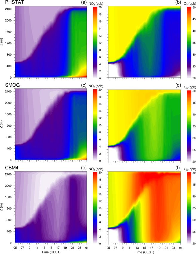
B. Khan et al.: Chemistry model for PALM model system 6.0                                                                  1173

systems which restricts their applicability on large domains      2     Model description
(Maronga et al., 2015, 2019).
   This paper describes the chemistry model that has been         2.1    PALM and PALM-4U
implemented in the PALM model system 6.0 as part of
PALM-4U (PALM for urban applications) components. In              The PALM model system 6.0 consists of the PALM core
the past PALM has been used to study urban turbulence             and PALM-4U (PALM for urban applications) components
structures (Letzel et al., 2008). Some studies also investi-      (Maronga et al., 2020) that have been added to PALM under
gated dispersion of reactive pollutants (NO, NO2 and O3 )         the MOSAIK (model-based city planning and application in
using simple steady-state chemistry in PALM in the urban          climate change) project (Maronga et al., 2019), one of which
street canyons (Cheng and Liu, 2011; Park et al., 2012; Han       is the chemistry module described in this paper. PALM solves
et al., 2018, 2019). The PALM-4U components are essen-            the non-hydrostatic, filtered, incompressible Navier–Stokes
tially designed for urban applications and offer several fea-     equations on a Cartesian grid in Boussinesq-approximated
tures required to simulate urban environments such as an en-      form for up to seven prognostic variables: the three veloc-
ergy balance solver for urban and natural surfaces, radiative     ity components (u, v, w) on a staggered Arakawa C grid and
transfer in the urban canopy layer, biometeorological anal-       four scalar variables, namely potential temperature (θ ), water
ysis products, self-nesting to allow very high resolution in      vapour mixing ratio (qv ), a passive scalar s and the subgrid-
regions of special interest, atmospheric aerosols, and gas-       scale turbulent kinetic energy (SGS-TKE) e (in LES mode)
phase chemistry (Raasch and Schröter, 2001; Maronga et al.,       (Maronga et al., 2019, 2020).
2015, 2020).                                                          By default, these SGS terms are parameterized using a 1.5-
   In order to offer the latter feature, an “online” coupled      order closure after Deardorff (1980). The model uses a fifth-
chemistry model has been implemented in the PALM model,           order advection scheme of Wicker and Skamarock (2002)
which is presented in this paper. The chemistry model in-         and a third-order Runge–Kutta scheme for time-stepping.
cludes chemical transformations in the gas phase, a simple        Monin–Obukhov similarity theory (MOST) is assumed be-
photolysis parameterization, dry deposition processes and an      tween every individual surface element and the first compu-
emission module to read anthropogenic pollutant emissions.        tational grid level. For details on meteorological and urban
The gas-phase chemistry has been implemented using the Ki-        climate features and available parameter options, see Resler
netic PreProcessor (KPP) (Damian et al., 2002) allowing au-       et al. (2017) and Maronga et al. (2020). Additionally, PALM
tomatic generation of the corresponding model code in order       includes options of fully interactive surface and radiation
to obtain the necessary flexibility in the choice of chemical     schemes, and a turbulence closure based on the RANS mode.
mechanisms. Due to the very high computational demands            Details of the dynamic core of the model are described in
of an LES-based urban climate model, this flexibility with re-    Maronga et al. (2015, 2020).
spect to the degree of detail of the gas-phase chemistry mech-
anism is of critical importance. A number of ready-to-use         2.2    The chemistry model
chemical mechanisms with varying complexity and detail are
supplied with PALM. Furthermore, the gas-phase chemistry          Atmospheric chemistry is integrated into the PALM code as
is coupled to the aerosol module SALSA (a sectional aerosol       a separate module (Fig. 1) that utilizes the meteorological
module for large-scale applications; Kokkola et al., 2008) im-    fields of PALM as input. Chemistry is coupled “online” with
plemented in PALM (Kurppa et al., 2019), which includes a         the PALM model; i.e. the prognostic equations for the chem-
detailed description of the aerosol number size distribution,     istry compounds are solved consistently with the equations
chemical composition and aerosol dynamic processes.               for momentum, heat and water constituents. This implemen-
   The analysis provided in this work is mostly qualitative       tation of chemistry allows for a future consideration of the
and intended to show the first applications of the chemistry      impact of trace gases and aerosol particles on meteorology by
model in a real urban environment, thereby demonstrating          radiative effects and aerosol–cloud interactions. As shown in
its capabilities and its flexibility. A detailed description of   Fig. 1 the main chemistry driver module calls and exchanges
the chemistry model and its implementation to PALM is pro-        data with separate modules for the chemistry solver, photol-
vided in Sect. 2. The model application and details of the nu-    ysis, handling of lateral boundary conditions, concentration
merical set-up for a case study representing a selected area      changes due to emissions and deposition.
in central Berlin, Germany, are described in Sect. 3, whereas        Depending on the need, a user can select a chemistry
results of the application of the chemistry model and com-        mechanism of different complexity. The Fortran code for the
parison of simulation results with observations are provided      selected gas-phase chemistry mechanism is generated by a
in Sect. 4. In the end, concluding remarks are provided in        preprocessor based on KPP (Damian et al., 2002). The latter
Sect. 5.                                                          is described in more detail in Sect. 2.2.2. Besides chemical
                                                                  transformations in the gas phase and a simple photolysis pa-
                                                                  rameterization (Sect. 2.2.3) the chemistry module includes
                                                                  dry deposition (Sect. 2.2.5), an interface to the aerosol mod-

https://doi.org/10.5194/gmd-14-1171-2021                                            Geosci. Model Dev., 14, 1171–1193, 2021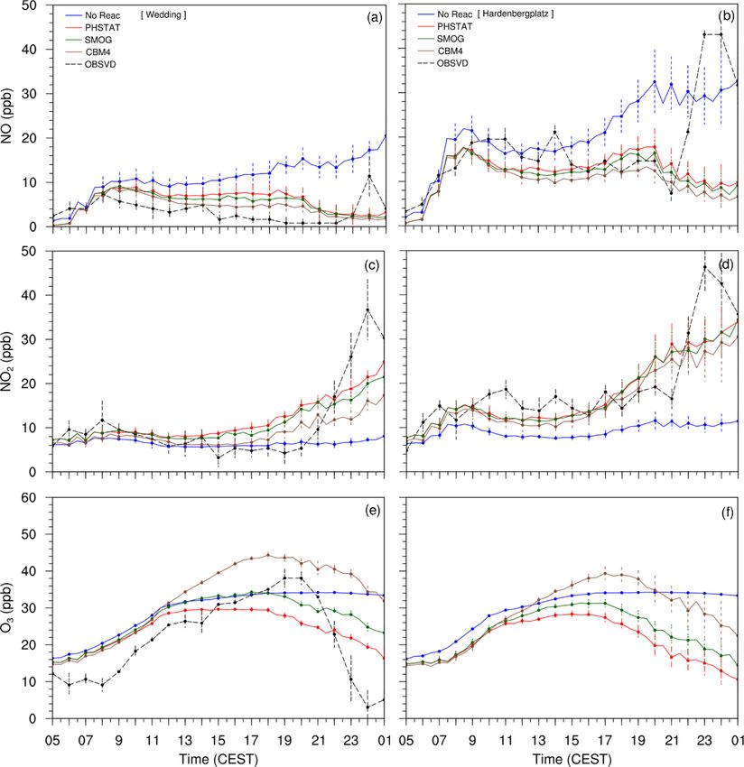
1174                                                               B. Khan et al.: Chemistry model for PALM model system 6.0

                                                                      reactions the rates are dependent on temperature and pres-
                                                                      sure. The last term in Eq. (1) (9n ) stands for sources (i.e.
                                                                      emissions) and sinks (i.e. deposition and scavenging). The
                                                                      number of prognostic equations depends on the number of
                                                                      species included in the chemical mechanism, and it is de-
                                                                      termined automatically during the KPP preprocessing step
                                                                      (Sect. 2.2.2).

                                                                      2.2.2   Gas-phase chemistry implementation

                                                                      The Fortran subroutines for solving the chemical reactions of
                                                                      a given gas-phase chemistry mechanism are generated auto-
                                                                      matically with the KPP, version 2.2.3 (Damian et al., 2002;
                                                                      Sandu et al., 2003; Sandu and Sander, 2006). KPP creates the
                                                                      code from a list of chemical reactions that represent a cer-
                                                                      tain chemical mechanism. Within the PALM environment,
                                                                      the subroutines with the integrator for the desired gas-phase
Figure 1. Schematic representation of the chemistry model (PALM-
4U component) of the PALM model system. The arrows show inter-        chemistry mechanism are generated by a preprocessor named
action between the PALM model core, the chemistry driver module       kpp4palm, which is based on the KP4 preprocessor (Jöckel
and sub-modules. The dashed box indicates the chemical prepro-        et al., 2010). As a first step, kpp4palm starts the KPP prepro-
cessor which generates subroutines to solve chemical reactions.       cessor. As a second step, the code from KPP is transformed
                                                                      into a PALM subroutine. As described by Jöckel et al. (2010),
                                                                      the preprocessing also includes an optimization of the LU
ule SALSA (Kurppa et al., 2019) (Sect. 2.2.4) and an option           (lower–upper) decomposition of the sparse Jacobian of the
for anthropogenic emissions (Sect. 2.3).                              ordinary differential equation system for the chemistry rate
                                                                      equations.
2.2.1   Prognostic equations
                                                                         KPP offers a variety of numerical solvers for the system of
When gas-phase chemistry is invoked, N additional prognos-            coupled ordinary differential equations describing the chemi-
tic equations are solved, with N being the number of variable         cal reactions. Tests comparing the performance of the Rosen-
compounds of the chemical reaction scheme. Except for the             brock solvers implemented in KPP have shown that the use
SGS flux terms, the overbar indicating filtered quantities is         of the most simple Rosenbrock solver, Ros-2, did not lead to
omitted to improve readability. The three-dimensional prog-           significantly different results than the use of the Rosenbrock
nostic equation for an atmospheric pollutant then reads as            solvers with higher orders (Sandu and Sander, 2006; Jöckel
follows:                                                              et al., 2010). Therefore, the Ros-2 solver was chosen as the
                                                                      default solver for the PALM-4U chemistry model.
                                  00
           1 ∂ ρ uj cn 1 ∂ ρ uj cn00

∂ cn                                     ∂ cn                            The automatic code generation by kpp4palm and KPP al-
      =−              −              +             + 9n ,
 ∂t       ρ ∂ xj        ρ ∂ xj            ∂ t chem                    lows for high flexibility in the choice of gas-phase chem-
          with i, j ∈ (1, 2, 3) ,                         (1)         ical mechanisms and numerical solvers. Since the number
                                                                      of chemical compounds of a mechanism from KPP is used
where cn (n = 1, N ) is the concentration of the respective air       to determine the number of prognostic equations (Eq. 1),
constituent, which can be either a reactive or passive gas-           it is also possible to add prognostic equations for an arbi-
phase species or an aerosol particulate matter compound. The          trary number of passive tracers by simply including reac-
term on the left-hand side is the total time derivative of the        tions of the form A → A in the list of chemical reactions,
pollutant concentration. The first two terms on the right-hand        which serves as input for KPP. For example, the passive
side represent the explicitly resolved and the SGS transport          tracer mechanism “passive” contains the following equations
of the scalar chemical quantity in x, y and z directions. A           in the passive.eqn file:
double prime indicates a SGS variable. The third term repre-          { 1.} PM10 = PM10 :                 1.0 ;
sents the change in concentration (cn ) of the trace gas n over       { 2.} PM25 = PM25 :                 1.0 ;
time due to production and loss to chemical reactions, which          (see Sects. S2–S9 of the Supplement for all .eqn files).
can be described as follows:

  ∂ cn
                                                                       The chemistry model includes a number of ready-to-use
             = φn (cm6=n ) + ϕn (cm6=n ) · cn ,             (2)       chemical mechanisms summarized in Table 1. The first two
   ∂t chem
                                                                      mechanisms describe only one or two passive tracers which
where φn and ϕn indicate the production and loss, respec-             represent PM10 and PM2.5 (particulate matter with the aero-
tively, of species n. For most of these production and loss           dynamic diameter ≤ 10 and ≤ 2.5 µm, respectively) with-

Geosci. Model Dev., 14, 1171–1193, 2021                                               https://doi.org/10.5194/gmd-14-1171-2021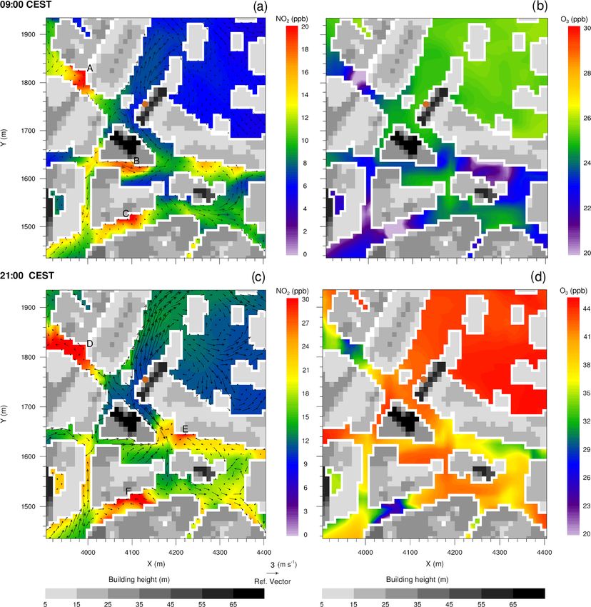
B. Khan et al.: Chemistry model for PALM model system 6.0                                                                1175

out any chemical transformations. As a representative of a      due to buildings, which is already implemented for the short-
“full” gas-phase mechanism, the well known Carbon Bond          wave radiation in the PALM-4U urban surface model but so
Mechanism 4 (CBM4) (Gery et al., 1989) is included. Al-         far not for the simple photolysis scheme.
though CBM4 has been replaced by the more detailed CB5
and CB6 mechanisms in the meantime, it is still applied in      2.2.4   Coupling to SALSA aerosol module
some models. The CBM4 mechanism was implemented in
the PALM model, since – with 32 compounds – it is the           The sectional aerosol module SALSA2.0 (Kokkola et al.,
smallest of the full mechanisms. Nevertheless, the compara-     2008) has recently been implemented into PALM, and a de-
tively large number of species precludes the use of the CBM4    tailed description is given in Kurppa et al. (2019). SALSA
mechanism for practical applications over larger domains.       describes the aerosol number size distribution, aerosol chem-
Therefore, we also included less computationally demanding      ical composition and aerosol dynamic processes. Currently,
mechanisms, such as the SMOG mechanism and its simpli-          the full SALSA implementation in PALM includes the fol-
fied version, the “SIMPLE” mechanism. By far, the photo-        lowing chemical compounds in the particulate phase: sul-
stationary equilibrium (PHSTAT mechanism) represents the        fate (SO2+4 ), organic carbon (OC), black carbon (BC), nitrate
most simple mechanism, consisting of only three species and     (NO−                       +
                                                                     3 ), ammonium (NH4 ), sea salt, dust and water (H2 O).
two reactions. The latter two mechanisms are also supplied      Aerosol particles can grow by condensation and dissolution
with an additional passive tracer which can be used to rep-     to liquid water of gaseous sulfuric acid (H2 SO4 ), nitric acid
resent PM10 (PHSTATP and SIMPLEP mechanisms). Three             (HNO3 ), ammonia (NH3 ), and semi- and non-volatile organ-
more mechanisms which can be used in combination with           ics (SVOCs and NVOCs), which establishes a link between
the sectional aerosol module SALSA (Kurppa et al., 2019)        SALSA and the chemistry module.
are described in Sect. 2.2.4.                                      SALSA is coupled to the gas-phase chemistry when the
   Two of the currently available mechanisms, SMOG and          gas-phase compounds listed above (H2 SO4 , HNO3 , NH3 ,
SIMPLE, include only major pollutants such as ozone (O3 ),      SVOCs and NVOCs) are either included in the gas-phase
nitric oxide (NO), nitrogen dioxide (NO2 ), carbon monoxide     chemistry scheme or are derived from prognostic variables
(CO), a highly simplified chemistry of volatile organic com-    of the gas-phase chemistry. Currently, PALM-4U includes
pounds (VOCs) and a very small number of products. For the      three different mechanisms in which SALSA is coupled
convenience of the users, it is not required to run kpp4palm    with the chemistry model. In the mechanisms “SALSAGAS”
for the ready-to-use mechanisms (Table 1) as their Fortran      and “SALSA+PHSTAT”, H2 SO4 , HNO3 , NH3 , SVOCs and
subroutines are already supplied with PALM. Currently, PH-      NVOCs are treated as passive compounds and are only
STATP is the default mechanism which will automatically         transported within the gas-phase chemistry model, whereas
be compiled with the rest of the PALM source code when          in “SALSA+SIMPLE”, HNO3 is formed by the reaction
the chemistry option is switched on. However, users can also    NO2 + OH → HNO3 . Additionally, any of the other mech-
add modified versions of the existing chemical mechanisms       anisms given in Table 1 or any user-supplied mechanism can
or define completely new mechanisms according to their spe-     also be coupled to SALSA.
cific needs.
                                                                2.2.5   Deposition
2.2.3   Photolysis frequencies
                                                                Deposition is a major sink of atmospheric pollutant con-
The parameterization of the photolysis frequencies is           centrations. Currently, only dry deposition processes are in-
adopted from the Master Chemical Mechanism (MCM) v3             cluded as precipitation (leading to wet deposition of pollu-
according to Saunders et al. (2003). Photolysis frequencies     tants) is not yet included in PALM. For dry deposition, a
are described as a function of the solar zenith angle ϑ and     resistance approach is taken where the exchange flux is the
three parameters, which are specific for each photolysis re-    result of a concentration difference between atmosphere and
action:                                                         earth surface and the resistance between them. Several path-
J = l (cos ϑ)m exp(−n sec ϑ) .                            (3)   ways exist for this flux, each with its own resistance and
                                                                concentration. The aerodynamic resistance depends mainly
Values for l, m and n are given for the relevant photolysis     on the atmospheric stability. In PALM, it is calculated via
reactions in Saunders et al. (2003) and on the MCM web          MOST, based on roughness lengths for heat and momentum
page (http://mcm.leeds.ac.uk/MCM/parameters/photolysis_         and the assumption of a constant flux layer between the sur-
param.htt, last access: 12 July 2020). Currently only a sim-    face and the first grid level.
ple parameterized photolysis scheme is available for photo-        For gases, the quasi-laminar layer resistance depends on
chemical reactions. More extensive photolysis schemes such      the atmospheric conditions and diffusivity of the deposited
as the Fast-J photolysis scheme (Wild et al., 2000) that are    gas, and it is calculated following Simpson et al. (2003). Fi-
based on the radiative transfer modelling will be included in   nally, the surface (canopy) resistance for gases, which is the
the future. These models will also make use of the shading      most challenging resistance to estimate due to the enormous

https://doi.org/10.5194/gmd-14-1171-2021                                          Geosci. Model Dev., 14, 1171–1193, 2021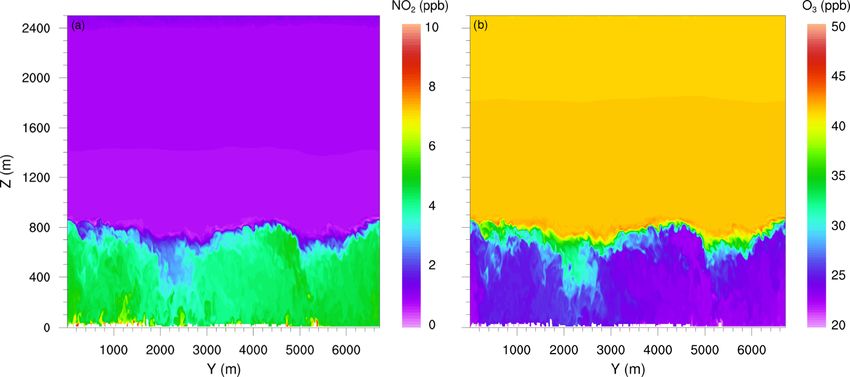
1176                                                                      B. Khan et al.: Chemistry model for PALM model system 6.0

Table 1. Description of built-in chemical mechanisms.

                      No.     Mechanism           Var.      Fixed                              KPP           Real       Photolysis
                                               species      species                        reactions     reactions
                      1       PASSIVE1                1     –                                      1a             0               0
                      2       PASSIVE                 2     –                                      2b             0               0
                      3       PHSTAT                  3     –                                       2             2               1
                      4       PHSTATP                 4     –                                      3a             2               1
                      5       SIMPLE                  9     water vapour                            7             7               2
                      6       SIMPLEP                10     water vapour                           8a             7               2
                      7       SMOG                   13     water vapour, O2 , CO2                 12            12               2
                      8       CBM4                   32     water vapour                           81            81              11
                    a Includes one passive compound which is realized in the KPP environment by the “reaction” PM → PM . b Includes
                                                                                                                 10   10
                    passive compounds which are realized in the KPP environment by the “reactions” PM10 → PM10 and PM2.5 → PM2.5 .

diversity of surfaces, is calculated using the DEPAC mod-                       levels of detail (LODs), depending on the amount of infor-
ule (Van Zanten et al., 2010). DEPAC is widely used in the                      mation available at the user’s disposal. With LOD 0 (“PA-
flux modelling community (e.g. Manders et al., 2017; Sauter                     RAMETERIZED”, mode), traffic emissions are parameter-
et al., 2016). The surface resistance parameterizations are                     ized based on emission factors specific to particular street
different for different land use types defined in the model. In                 types. All street segments contained in the domain will be
DEPAC, three deposition pathways for the surface resistance                     classified into “main” and “side” street segments. A mean
are taken into account:                                                         surface emission flux tendency for each chemical species
                                                                                contained the active chemical mechanism, in kilograms per
  – through the stomata                                                         square metre per day, and will be provided together with
  – through the external leaf surface                                           a weighting factor for main- and side-street emissions in
                                                                                the PALM parameter file. Street type classification based
  – through the soil.                                                           on OpenStreetMap definitions (OpenStreetMap contributors,
                                                                                2017) is to be included in the PALM static driver (Maronga
DEPAC is extensively described in a technical report by Van
                                                                                et al., 2020). A diurnal profile derived from traffic counts is
Zanten et al. (2010). It also includes a compensation point
                                                                                implemented to disaggregate total emissions into hourly in-
for ammonia which is currently set to zero in PALM.
                                                                                tervals. Currently a default profile is applied to all species
   For the passive particulate matter in the chemistry model,
                                                                                for main and side street segments, and details can be found
the land-use-dependent deposition scheme of Zhang et al.
                                                                                in the online documentation for the PALM-4U chemistry
(2001) has been implemented into PALM. The formulations
                                                                                model (https://palm.muk.uni-hannover.de/trac/wiki/doc, last
have been chosen as they include an explicit dependence on
                                                                                access: 12 September 2020). Future plans include expansion
aerosol size. For particulate matter, the deposition velocity
                                                                                of the LOD 0 emission model to accommodate further modes
is calculated by the gravitational settling or sedimentation
                                                                                of anthropogenic emissions such as domestic heating. More
velocity (mainly relevant for the larger particles), the aero-
                                                                                detailed traffic emission data can be provided in gridded form
dynamic resistance (see above), and the surface resistance.
                                                                                in PALM-specific NetCDF files (Maronga et al., 2020). LOD
The sedimentation velocity mainly depends on particle prop-
                                                                                1 emissions are gridded annual emission data for each sector
erties, the gravitational acceleration and the viscosity coef-
                                                                                (e.g. industry, domestic heating, traffic), which will be tem-
ficient of air. The formulation for the surface resistance is
                                                                                porally disaggregated using sector-specific standard time fac-
empirical with parameters that are based on a few field stud-
                                                                                tors. With LOD 2, the user can introduce preprocessed grid-
ies including the collection efficiencies for Brownian diffu-
                                                                                ded emission data that are already temporally disaggregated,
sion, impaction and interception, respectively, and a correc-
                                                                                e.g. in hourly intervals.
tion factor representing the fraction of particles that stick to
the surface depending on the surface wetness. Further details
                                                                                2.4    Initial and boundary conditions
can be found in Zhang et al. (2001).

2.3    Traffic emissions                                                        Lateral boundary conditions for chemical compounds can
                                                                                be chosen in the same way as the lateral boundary condi-
The chemistry model of PALM-4U includes a module for                            tion for other scalars, e.g. potential temperature, being ei-
reading gaseous and passive anthropogenic emission input                        ther cyclic conditions or non-cyclic (Maronga et al., 2020).
from traffic sources and converting it to the appropriate for-                  In most urban applications, chemistry requires non-cyclic
mat. These emission data can be provided in three possible                      boundary conditions, because cyclic conditions lead to accu-

Geosci. Model Dev., 14, 1171–1193, 2021                                                              https://doi.org/10.5194/gmd-14-1171-2021
B. Khan et al.: Chemistry model for PALM model system 6.0 1177
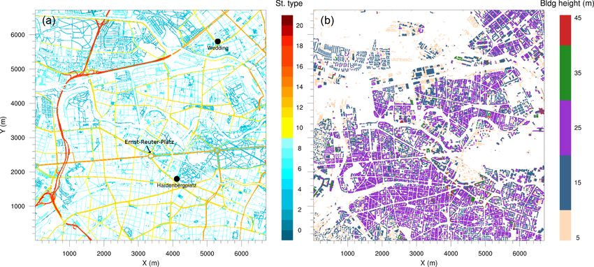
mulation of pollutants to the modelling domain if pollutant The topographic data with streets, buildings, water bod-
emissions exist. As part of the PALM-4U components, nest- ies, vegetation and other urban land surface features at a
ing has been implemented to the chemistry module. In offline 10 m resolution have been processed for Berlin by the Ger-
nesting, PALM can be coupled to a larger-scale (mesoscale, man Space Agency (DLR) (Heldens et al., 2020). The street
regional or global) model to provide dynamic boundary con- types shown in Fig. 2a are based on OpenStreetMap (Open-
ditions for the meteorological variables as well as air pollu- StreetMap contributors, 2017). The model domain includes
tants. As larger-scale models do not fully resolve turbulence, 13 types of one-way and two-way roads. The building height
a synthetic turbulence inflow generator has been introduced data are based on CityGML data from FIS Broker Berlin
(Gronemeier et al., 2015). (Senatsverwaltung für Stadtentwicklung und Wohnen, 2020)
Initial concentrations of primary compounds to control the (Fig. 2b). With the exception of 10 buildings with a height be-
chemistry model are controlled by the chemistry name list tween 45 and 65 m and two buildings which are higher than
”&chemistry_parameters” in the PALM parameter file. Op- 70 m, the building heights in the simulation domain are be-
tions for prescribing initial conditions are available for both tween 5 and 45 m.
surface initial conditions and initial vertical profiles for the The simulation domain contains five types of vegetation
area or region of interest. There are no default initial con- categories that include grass and shrubs of different height.
centrations and the user is responsible for providing these Trees resolved by the canopy model are characterized by the
values based on, for example, the measured background con- three-dimensional leaf area density (LAD) per unit volume.
centration of primary chemical compounds for whom initial For the model configuration used here, LAD is considered
concentrations are defined. These primary compounds must for a maximum height of up to 40 m above the ground and
be part of the applied chemical mechanism. assumes values up to 3.1 m2 m−3 with an average value of
0.44 m2 m−3 . Lake, river, pond and fountain categories are
included in the domain for water types. Considering the ur-
3 Chemistry model application ban surface, soil type of the entire domain is classified as
“coarse”, whereas pavement types in the domain are defined
In order to demonstrate the ability of the chemistry imple-
with six different categories of asphalt, concrete and stones.
mentation, we performed simulations for an entire daily cy-
cle in a realistic urban environment and compared simulation
3.2 Observational data
results against observational data. To analyse the effect of
different chemical mechanisms with different complexity on
In addition to routine observations of near-surface tempera-
the resulting concentrations, we performed simulations with
ture, cloud cover, and wind speed and direction at the Berlin
three chemical mechanisms and one passive case where only
Tegel airport from the open-access Climate Data Center
transport and dry deposition were considered.
(CDC) of the German Weather Service (Deutscher Wetterdi-
3.1 Modelled episode and modelling domain enst, 2020), we also analysed radiosonde data from Linden-
berg (Oolman, 2017) and aerosol backscatter observations
The model was run for 24 h from 00:00 to 24:00 UTC for from a ceilometer for 16 and 17 July 2017 to understand
17 July 2017 (02:00 Central European Summer Time (CEST) the vertical structure of the atmosphere in the area of inter-
17 July 2017 to 02:00 CEST 18 July 2017) for a city quarter est. Ceilometer observations of aerosol back-scatter profiles
located around the Ernst-Reuter-Platz in Berlin, Germany. were performed on the roof of the Charlottenburg building of
This particular day was chosen as it represents an “ideal” the Technical University of Berlin (52.5123◦ N, 13.3279◦ E)
Berlin summer day with mostly clear sky, some scattered as part of the Urban Climate Observatory (UCO) operated
clouds in the morning after a partly cloudy night, and only a by the Chair of Climatology at Technische Universität Berlin
few passing clouds in the afternoon. The temperature ranged for long-term observations of atmospheric processes in cities
between 289 and 298 K with moderate winds predominantly (Scherer et al., 2019a; Wiegner et al., 2002) and contributed
from westerly direction. 17 July 2017 was a Monday; there- to the research program Urban Climate Under Change [UC]2
fore, the diurnal cycle of the traffic emissions can be de- (Scherer et al., 2019b). Mixing layer heights were derived
scribed as a typical weekday with relative maxima during from the aerosol backscatter signal according to Geiß et al.
the morning and evening rush hours. (2017).
Figure 2 shows the computational domain that covers an Observations from radiosondes and ceilometers indicate
area of 6.71 km × 6.71 km (671 × 671 grid points) with a strong showers during the previous days that resulted in a
model top at 3.6 km above the surface. The horizontal grid very well mixed (almost moist adiabatic) layer in the lower
spacing in x and y direction is 10 m. In the vertical, with 312 troposphere that lead to an almost constant potential temper-
layers, the grid spacing is 10 m up to 2700 m, above which it ature gradient above the inversion; therefore, there was no
increases by an expansion factor of 1.033 until the grid spac- residual layer at midnight on 17 July, when the model was
ing in the z direction reaches 40.0 m. initialized for a 24 h run. The ceilometer observations for
17 July 2017 also did not show disturbances by clouds; the
https://doi.org/10.5194/gmd-14-1171-2021 Geosci. Model Dev., 14, 1171–1193, 2021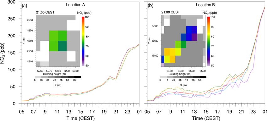
1178                                                               B. Khan et al.: Chemistry model for PALM model system 6.0

Figure 2. Simulation domain: (a) street type, (b) building height. The black dots show the location of the observational monitoring stations
Wedding and Hardenbergplatz.

mixed-layer top, however, remained below 2000 m through-                made available on the Senate department web pages (Senate-
out the diurnal cycle.                                                  Berlin, 2017).
   The air quality measurements that are compared with the
simulations are conducted at automated stations of the so-              3.3    Model configuration and initialization
called BLUME network of the Berlin Department for the En-
vironment, Transport and Climate Protection (Senate-Berlin,             The PALM model system, version 6.0, revisions 4450 and
2017). Two stations, Wedding and Hardenbergplatz (Fig. 2),              4601 (only for flux profiles of chemical compounds), has
are located within the model domain. The average height of              been used in this study. A multigrid scheme has been used
the air quality sensors at both stations is 4 m above ground.           to calculate pressure perturbations in the prognostic equa-
   The roadside air quality station at Hardenbergplatz is lo-           tions for momentum (Maronga et al., 2015), and a third-order
cated at a busy junction with high traffic flow and in close            Runge–Kutta scheme (Williamson, 1980) has been used for
proximity to the train and bus stations. The station records            time integration. The advection of momentum and scalars
only NO and NO2 . The height of the buildings in the vicinity           was discretized by a fifth-order advection scheme by Wicker
of the station ranges from 10 to 30 m. The dense road net-              and Skamarock (Wicker and Skamarock, 2002). Following
work of small and big streets to the north, south and west              Skamarock (2006) and Skamarock and Klemp (2008), we
of the station warrants transport of traffic-related pollutants         employed a monotonic limiter for the advection of chemical
towards Hardenbergplatz when the station is located down-               species along the vertical direction in order to avoid unreal-
wind of these directions. To the north-east of the station is           istically high concentrations within the poorly resolved cav-
the Berlin Zoo and Tiergarten park that spread over 5.2 km2 .           ities (e.g. courtyards represented by only a few grid points)
Thus, with a NE flow, the Hardenbergplatz air quality sta-              which can occasionally occur due to stationary numerical os-
tion would be downwind of the large vegetated area, and less            cillations near buildings. Rayleigh damping has been used
anthropogenic pollutants would be advected to the station,              above 2500 m in order to weaken the effect of gravity waves
although the concentration of biogenic volatile organic com-            above the boundary-layer top.
pounds (BVOCs) is expected to be larger.                                   The Rapid Radiative Transfer Model (RRTMG) (Clough
   The background air quality station of Wedding is located             et al., 2005), which is included in PALM, has been used
to the north in the outskirts of the city away from heavy               to calculate radiation fluxes and radiation heating rates.
traffic flow. Wedding air quality station records PM10 , NO,            Natural-type surfaces are treated by the land-surface model
NO2 and O3 . The city centre is located to the south of the             of PALM, while building surfaces are treated by the urban-
station, so the station would likely record higher levels of            surface model (Resler et al., 2017; Maronga et al., 2020). The
NOx and PM10 during southerly flow. Both stations collect               surface roughness length is set according to the given build-
data every 5 min which are then averaged to hourly data and             ing, vegetation, pavement and water types and based on the
                                                                        information from the static driver. The MOST then provides

Geosci. Model Dev., 14, 1171–1193, 2021                                                   https://doi.org/10.5194/gmd-14-1171-2021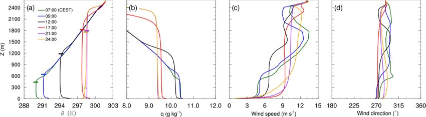
B. Khan et al.: Chemistry model for PALM model system 6.0                                                                   1179

surface fluxes of momentum (shear stress) and scalar quan-        put of the operational mesoscale weather prediction model
tities (heat, moisture) at the lower boundary condition. The      COSMO-DE/D2 (COnsortium for Small-scale MOdelling;
application of MOST assumptions on urban surfaces has not         Baldauf et al., 2011) for 17 July 2017. The INIFOR tool was
been thoroughly evaluated. However, similar studies, for ex-      used to prepare these initial conditions in a format that can
ample Letzel et al. (2008) and Gronemeier et al. (2020), show     be read by PALM (Kadasch et al., 2020). The initial profiles
that LES results were in good agreement with wind-tunnel          of pollutant concentration are based on the mean observed
data representing an urban setting. Based on these findings,      near-surface concentrations of NO, NO2 and O3 from the
it is assumed that MOST is applicable in the simulated urban      stations of the BLUME network (Sect. 3.2). Initial concen-
surface.                                                          trations of NO, NO2 and O3 above 495 m were set to 0.0,
    Three chemical mechanisms, namely PHSTAT, SMOG                2.0 and 40.0 ppb respectively. Considering the strong impact
and CBM4, along with one no-reaction case have been ap-           of traffic emissions on local pollutant concentrations, all grid
plied (Table 1). The CBM4 (Gery et al., 1989) mechanism is        points of the model domain were initialized with identical
the most complex mechanism currently included in PALM-            pollutant profiles.
4U. It includes VOC and HOx (hydrogen oxide radicals),                At the lateral boundaries, cyclic boundary conditions are
chemistry and formation of ozone, and further photochemi-         applied for the velocity components, θ , q and the chemi-
cal products. Assuming that the CBM4 is more accurate than        cal compounds. The application of cyclic boundary condi-
the more simple mechanisms due to its more complete rep-          tions may be justified by low variability in wind direction
resentation of atmospheric chemistry, the baseline simula-        with prevailing westerly winds throughout the major part of
tion of this study was performed with CBM4. The SMOG              17 July 2017 and the large extent of the urban area upwind of
photochemical mechanism was included for comparison as            the model domain. One main reason for not applying bound-
it contains a strongly simplified NOx –HOx –VOC chemistry         ary conditions from COSMO-DE/D2 was that it requires a
with VOC just described by one single representative com-         very large fetch to develop turbulence, as turbulence quan-
pound (Table 1). Due to a smaller number of species and           tities are not supplied by the boundary conditions from the
reactions, the SMOG mechanism is much faster compared to          mesoscale COSMO-DE/D2 simulation. Furthermore, chem-
the CBM4 mechanism. The objective of including the SMOG           istry fields for the lateral boundaries were not available from
mechanism was to assess computational efficiency at the cost      COSMO-DE/D2. Thus, cyclic boundary conditions were ap-
of accuracy of the description of the VOC chemistry. The          plied that ensure cyclic inflow of meteorological and chem-
most simple mechanism, PHSTAT, describes only the photo-          istry variables that left the domain from the opposite lateral
stationary equilibrium between NO, NO2 and O3 and does            boundary. Therefore, a continuous inflow and outflow of pol-
not include any VOC chemistry or formation of any sec-            lutants in and out of the simulation domain is assumed. This
ondary compounds besides ozone. In a fourth experiment,           is reasonable, as the simulation domain is located in the mid-
the photostationary mechanism (PHSTAT) was applied with           dle of a large highly urbanized area.
the gas-phase chemistry turned off; i.e. the chemical com-            At the bottom boundary, a Dirichlet condition is applied
pounds were treated as passive tracers and only transport and     to flow, θ and q, whereas a Neumann condition is applied
dry deposition were allowed.                                      to e, p and chemical compounds. Moreover, a canopy drag
    Only traffic emissions, which are parameterized de-           coefficient Cd = 0.3 has been applied while the roughness
pending on the street type (“PARAMETERIZED” option,               is specified internally depending on vegetation type. At the
LOD=0), were considered. Since the area of interest is in         top boundary, Dirichlet boundary conditions are applied to
the inner part of the city with many major roads, and domes-      flow and p only, and initial gradient is applied to θ while
tic heating emissions are neglectable in July, this restriction   Neumann boundary conditions are applied to q and chemical
seems justified. The traffic emissions of the “PARAMETER-         compounds.
IZED” option are based on emission factors derived from
HBEFA (HandBook Emission FActors road transport; Haus-
berger and Matzer, 2017) and traffic counts provided by the       4   Results and discussion
Senate Department for the Environment, Transport and Cli-
                                                                  The results of the chemistry model simulations are pre-
mate Protection of Berlin. A mean surface emission of 4745
                                                                  sented for 20 h from 03:00 UTC (05:00 CEST) to 23:00 UTC
and 1326 µmol m−2 d−1 is applied for NO and NO2 , respec-
                                                                  (01:00 CEST 18 July 2017). All plots and data in this case
tively, and weights of 1.667 for main streets and 0.334 for
                                                                  study are presented in CEST. The simulation output was ex-
side streets are applied for the current study. Considering the
                                                                  ported to file every 10 min as instantaneous values and ev-
diurnal cycle of emissions a typical temporal profile of traf-
                                                                  ery 30 min as temporal averages. Since observational data are
fic emissions (see Sect. S1 of the Supplement), with maxima
                                                                  available in hourly averaged data, we used the 30 min aver-
at 08:00 and 18:00–19:00 CEST based on traffic counts at
                                                                  aged model data for comparison with observations. For all
Ernst-Reuter-Platz, was applied.
                                                                  other plots we used instantaneous data.
    As initial conditions profiles of θ , q, u, v and w, soil
moisture and soil temperature were obtained from the out-

https://doi.org/10.5194/gmd-14-1171-2021                                            Geosci. Model Dev., 14, 1171–1193, 2021
1180 B. Khan et al.: Chemistry model for PALM model system 6.0
4.1 Meteorology mixing during further growth of the mixed layer as well as
the fast reaction with O3 (Reaction R1). The NO concentra-
Figure 3 shows vertical profiles of potential temperature, tions above the inversion are much lower and mostly influ-
mixing ratio, wind speed and wind direction over the diur- enced by the background levels thus making NO vertical flux
nal cycle. The profiles of potential temperature indicate a positive (Fig. 4e) showing upward transport of NO.
vertically well mixed boundary layer during daytime, evolv- Unlike NO, the NO2 concentration profiles in Fig. 4b
ing from approximately 500 m at 07:00 CEST to more than show only small differences in the morning hours (07:00 and
2300 m at 21:00 CEST, while in the evening hours the near- 09:00 CEST). In the afternoon (12:00 and 17:00 CEST) when
surface layer stabilizes. The mixed-layer depth agrees fairly the convection is stronger, the NO2 concentration is the low-
well with the observed values from ceilometer measurements est due to the combined effect of upward vertical mixing in-
(horizontal bars in Fig. 3a), except for the late afternoon and dicated by Fig. 4f and photolysis of NO2 (Reaction R2).
evening hours, where the modelled boundary-layer depth is Reactions (R1)–(R3) between NO, NO2 and O3 do not re-
over-predicted by up to 15 %. This can have various causes; sult in a net gain of O3 unless additional NO2 is supplied (e.g.
e.g. in our simulations we neglected larger-scale processes primary NO2 from traffic emissions) and O3 is formed by Re-
such as subsidence or mesoscale advection. The wind comes actions (R2) and (R3). However, OH radical chain reactions
from westerly directions at a mean wind speeds of about 6– of VOCs result in the formation of excess NO2 (Reactions R4
9 m s−1 within the mixed layer. and R5) and thus O(3 P) (Reaction R2), which results in a net
O3 gain (Cao et al., 2019). In a schematic form, the formation
4.2 Vertical mixing of NO2 and O3 of NO2 due to VOC oxidation can be summarized by
Figure 4 shows mean profiles of concentrations and verti- OH + RH + O2 → RO2 , (R4)
cal fluxes of NO, NO2 , O3 and CO for the selected times
of the diurnal cycle on 17 July 2017, simulated with the RO2 + NO → RO + NO2 , (R5)
CBM4 mechanism. Profiles and fluxes of CO are added to
where RH stands for any explicitly described or lumped non-
represent transport characteristics of passive species. Posi-
methane hydrocarbon and RO2 represents any organic per-
tive fluxes with a negative vertical gradient can be observed
oxy radical.
for NO and NO2 , indicating net upward transport of the re-
In addition to Reaction (R3), the O3 levels within the
spective compounds from the surface towards higher levels
mixed layer are also replenished through down-welling from
during the entire diurnal cycle. The emitted NO from traffic
above the inversion during the day, which is evident from the
sources oxidized to NO2 by reaction with the available O3 :
negative flux profiles of O3 (Fig. 4g). As a result O3 con-
NO + O3 → NO2 + O2 . (R1) centration gradually increased from 18 ppb at 07:00 CEST to
43 ppb at 17:00 CEST.
This leads to an increase in NO2 and a decrease in O3 within In the evening hours (21:00 CEST onward), the NO con-
the boundary layer. As indicated by Fig. 4g the growth of the centration is reduced to 1 ppb near the surface while it is
boundary layer after sunrise leads to downward transport of completely removed from the residual layer. In the reduced
O3 since ozone concentrations in the residual layer are higher (no) solar radiation, NO2 photolysis (Reaction R2) slows
than within the mixed layer. At the same time, photolysis of down (stops), whereas emission and a limited Reaction (R1)
NO2 (Reaction R2) and photochemical formation of O3 (Re- reaction (because of very low available NO) favours an in-
action R3) by VOC chemistry retained and slightly increased crease in the NO2 mixing ratio. This resulted in the highest
the O3 concentration within the boundary layer as well as in near-surface NO2 concentrations at 24:00 CEST in the noc-
the residual layer. turnal stable layer. In the well mixed residual layer above, the
NO2 concentration at 24:00 CEST is up to 1 ppb lower than
NO2 + hν → NO + O(3 P) (R2) NO2 concentrations at 21:00 CEST. Ozone is also reduced to
3
O2 + O( P) + M → O3 + M (R3) 3 ppb at 24:00 CEST but remains well mixed in the residual
layer above the shallow nocturnal stable boundary layer. Car-
Near-surface concentrations of NO are 1 to 2 ppb higher bon monoxide has been added to the analysis as a proxy to
than the remaining mixed layer throughout the diurnal passive species (Fig. 4d). In the morning hours, the concen-
course. At 09:00 CEST, owing to emissions from traffic tration is highest, then it gradually decreases due to turbulent
sources, the NO concentration increases from 3 to 5 ppb in mixing in the rapidly growing mixed layer and partly due to
the first few metres above the surface then evenly dilutes in dry deposition.
the shallow mixed layer and stabilizes with a mixing ratio of Figure 5 shows YZ vertical cross sections at Hardenberg-
3 ppb. Besides the high NOx emissions in the morning hours, platz for NO2 and O3 . Turbulence and the growth of the
this increase can also be attributed to the onset of NO2 pho- mixed-layer height caused downward vertical mixing and O3
tolysis (Reaction R2). During the rest of the day, NO concen- entrainment near the boundary-layer top that resulted in in-
trations gradually reduces, mostly due to dilution by vertical crease in O3 concentration as well as in a decrease in NO2
Geosci. Model Dev., 14, 1171–1193, 2021 https://doi.org/10.5194/gmd-14-1171-2021B. Khan et al.: Chemistry model for PALM model system 6.0 1181
Figure 3. Vertical profiles of (a) potential temperature, (b) mixing ratio, (c) wind speed and (d) wind direction, at different times from
morning to midnight on 17 July 2017. The horizontal bars in (a) indicate the boundary-layer height derived from ceilometer observations.
Figure 4. Mean vertical profiles of species concentration for (a) NO, (b) NO2 , (c) O3 and (d) CO, as well as their total vertical fluxes (e–h)
over the diurnal cycle on 17 July 2017, simulated with the CBM4 mechanism.
concentrations to 2.0 ppb. Near the ground, the NO2 concen- (not shown), which are emitted by road traffic, were high in
tration is still of the order of 10 ppb. At the top of the bound- the morning and evening hours due to stable conditions and
ary layer, the concentration of OH and HO2 were higher than high emissions.
in the surrounding areas, which indicates active NOx –VOC– Most of the high NO2 concentrations in the morning hours
O3 chemistry in the turbulent entrainment zone. (Fig. 6a) are predicted in the street canyons in the south-
ern part of the simulation domain, where numerous buildings
4.3 Spatial distribution of pollutants with a height of approximately 20 m are present (see Fig. 2a).
In the street canyons of this area, wind speeds of less than
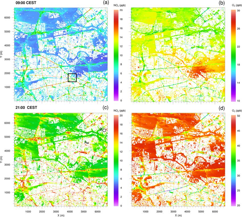
The spatial distribution of NO2 and O3 concentrations 5 m 2 m s−1 were simulated below 20 m, while wind speeds were
above the surface (Fig. 6) are discussed for 09:00 and almost twice as high over the open areas in the northern part
21:00 CEST as simulated with the CBM4 mechanism. The of the model domain (not shown). Therefore, emitted NOx
concentrations of NOx , aldehyde and hydrocarbon species
https://doi.org/10.5194/gmd-14-1171-2021 Geosci. Model Dev., 14, 1171–1193, 20211182 B. Khan et al.: Chemistry model for PALM model system 6.0 Figure 5. YZ vertical cross sections of NO2 and O3 (drawn through Hardenbergplatz, Fig. 2a), simulated with the CBM4 mechanism at 09:00 CEST on 17 July 2017. is more diluted by advection over the open areas. Further- creased to 20 ppb. However, in the open spaces and over veg- more, in the morning hours compared to the open spaces, etation with very low NO, the O3 concentration is of the order vertical mixing and transport in the street canyons is inhib- of 50 ppb. ited mainly due to delayed heating of the ground, which is To provide an overview of the pollutant dispersion at attributed to the shading of the surrounding buildings. There- the street level, a small section of the model domain fore, O3 is predominantly titrated by Reaction (R1) (Fig. 6b) (500 × 500 m) in the Hardenbergplatz area has been analysed over the road network reducing its concentration to the order (Fig. 7). This small urban section is characterized by a typical of 20 ppb, while over open spaces and vegetation (especially urban environment with streets, paved areas, buildings with the southern part of the Tiergarten) a slightly higher O3 mix- varying heights and some vegetated areas of the Tiergarten ing ratio (27 ppb) is found. The initial O3 values near the sur- located to the north-east. The dispersion of air pollutants in face were set to 10 ppb increasing to 40 ppb around 500 m a street canyon generally depends on the aspect ratio (ratio above the surface. A higher concentration of O3 (30 ppb) of building height to street width) and rate at which the street near the surface in the open spaces indicates strong verti- exchanges air vertically with the above roof-level atmosphere cal mixing and downward transport of O3 in the morning and laterally with connecting streets (N’Riain et al., 1998). hours of the day. In the evening, however, the NO2 distri- Figure 7 shows the dispersion and chemical transformation bution is somewhat more uniform over the entire road net- of NO2 and O3 in the street canyons and surrounding ar- work (Fig. 6c). This is attributed to emissions from traffic eas. The vegetated area of the Tiergarten north-east of the with reduced or absent photolysis of NO2 (Reaction R2) and domain has relatively high O3 levels and small NO2 con- titration of O3 . Under the low-wind conditions below 50 m, centrations, which is attributed to the low NO concentrations ventilation is reduced and leads to an increase in NO2 over over the vegetation that lead to reduced O3 titration (Reac- street crossings and main and side roads. Consequently, the tion R1). The model has emissions only from traffic sources, NO2 concentration increased by 30 % in the evening hours and therefore availability of the primary species other than over roads and adjacent paved areas, whereas over the vege- roads depends upon the dispersion of the primary chemical tated areas (grass, crops, shrubs and trees), NO2 concentra- compounds such as NO. In the street canyons, O3 is titrated tions were around 5 ppb in the morning hours and reached up by NO by Reaction (R1) resulting in production of NO2 . to 10 ppb in the evening hours. The daytime NOx –O3 –VOC In the morning hours, NO2 concentration increases in chemistry resulted in elevated O3 levels which increased by some sections of the street canyons (locations A, B and C more than 100 % as compared to the morning concentrations, in Fig. 7a) which are located to the west/southwest of the mostly due to photochemical production of O3 (Reactions tall buildings and thus lie under the shade of the building R2 and R3) during daytime. In the evening hours (Fig. 6d), structures. Due to the particular street geometry, and flow O3 is largely titrated by Reaction (R1) over the road net- dynamics above the urban canopy, these sections also ex- work. In certain sections of the street canyons where micro- perience weak wind conditions. The elevated NO2 concen- meteorological conditions are more favourable, O3 levels de- trations are due to later onset of the turbulence and vertical Geosci. Model Dev., 14, 1171–1193, 2021 https://doi.org/10.5194/gmd-14-1171-2021
You can also read