FALL3D-8.0: a computational model for atmospheric transport and deposition of particles, aerosols and radionuclides - Part 1: Model physics and ...
←
→
Page content transcription
If your browser does not render page correctly, please read the page content below
Geosci. Model Dev., 13, 1431–1458, 2020
https://doi.org/10.5194/gmd-13-1431-2020
© Author(s) 2020. This work is distributed under
the Creative Commons Attribution 4.0 License.

FALL3D-8.0: a computational model for atmospheric transport and
deposition of particles, aerosols and radionuclides –
Part 1: Model physics and numerics
Arnau Folch1 , Leonardo Mingari1 , Natalia Gutierrez1 , Mauricio Hanzich1 , Giovanni Macedonio2 , and Antonio Costa3
1 CASE    Department, Barcelona Supercomputing Center, Barcelona, Spain
2 Istituto Nazionale di Geofisica e Vulcanologia, Osservatorio Vesuviano, Naples, Italy
3 Istituto Nazionale di Geofisica e Vulcanologia, Sezione di Bologna, Bologna, Italy

Correspondence: Arnau Folch (afolch@bsc.es)

Received: 4 November 2019 – Discussion started: 13 December 2019
Revised: 10 February 2020 – Accepted: 16 February 2020 – Published: 24 March 2020

Abstract. This paper presents FALL3D-8.0, the last ver-           1   Introduction
sion release of an open-source code with 15+ years of track
record and a growing number of users in the volcanolog-           FALL3D is an open-source offline Eulerian model for atmo-
ical and atmospheric communities. The code has been re-           spheric passive transport and deposition based on the so-
designed and rewritten from scratch in the framework of           called advection–diffusion–sedimentation (ADS) equation.
the EU Centre of Excellence for Exascale in Solid Earth           The model, originally developed for inert volcanic particles
(ChEESE) in order to overcome legacy issues and allow for         (tephra), has a track record of 50+ publications on differ-
successive optimisations in the preparation of the code to-       ent model applications and code validation, as well as an
wards extreme-scale computing. However, this baseline ver-        ever-growing community of users worldwide, including aca-
sion already contains substantial improvements in terms of        demic, private and research institutions and several institu-
model physics, solving algorithms, and code accuracy and          tions tasked with the operational forecast of volcanic ash
performance. The code, originally conceived for atmospheric       clouds. The first versions of FALL3D (v1.x series) appeared
dispersal and deposition of tephra particles, has been ex-        back in 2003 (Costa and Macedonio, 2004); at that time, the
tended to model other types of particles, aerosols and ra-        code was serial and written in Fortran 77. Code improve-
dionuclides. The solving strategy has also been changed,          ments at different levels have been continuously incorporated
replacing the former central-difference scheme for a high-        since then, including relevant milestones leading to code ver-
resolution central-upwind scheme derived from finite vol-         sion upgrades, e.g. the coupling with 1-D buoyant plume the-
umes, which minimises numerical diffusion even in the pres-       ory (BPT) models to define eruption column sources (v2.x,
ence of sharp concentration gradients and discontinuities.        2004), the introduction of the Lax–Wendroff (LW) central-
The parallelisation strategy, input/output (I/O), model pre-      difference scheme for solving the ADS equation (v3.x, 2005)
process workflows and memory management have also been            and other algorithmic improvements (Costa et al., 2006), full
reconsidered, leading to substantial improvements on code         code rewriting in Fortran 90 and distributed memory par-
scalability, efficiency and overall capability to handle much     allelisation by means of Message Passing Interface (MPI)
larger problems. All these new features and improvements          (v5.x, 2007), first implementations of operational workflows
have implications on operational model performance and al-        to forecast ash cloud dispersal and fallout (Folch et al., 2008,
low, among others, adding data assimilation and ensemble          2009), and several other improvements (e.g. de la Cruz et al.,
forecast in future releases. This paper details the FALL3D-       2016) until the v7.3.4 release in 2018.
8.0 model physics and the numerical implementation of the            Along these 15+ years, FALL3D has been used in multi-
code.                                                             ple applications (e.g. Folch, 2012) including, among others,
                                                                  assessment of hazards from tephra fallout at different vol-

Published by Copernicus Publications on behalf of the European Geosciences Union.
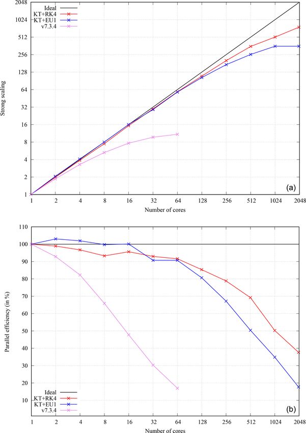
1432                                                                                      A. Folch et al.: FALL3D-8.0 – Part 1

canoes (e.g. Scaini et al., 2012; Selva et al., 2014; Sandri       comparison of model performance and scalability with re-
et al., 2016), impacts of ash cloud dispersal on civil aviation    spect to v7.x. This paper shows only one illustrative exam-
(e.g. Sulpizio et al., 2012; Bonasia et al., 2013; Biass et al.,   ple of FALL3D-8.0 model results for ash dispersal from the
2014; Scaini et al., 2014), obtaining relevant eruption source     2011 Cordón Caulle eruption. A companion paper (Prata
parameters (e.g. Folch et al., 2012; Parra et al., 2016; Poret     et al., 2020) contains the second part, including a detailed
et al., 2017), impacts of past super-eruptions on climate, en-     FALL3D-8.0 model validation for several simulations that
vironment and humans (e.g. Costa et al., 2012, 2014; Martí         are part of the new benchmark suite of the code. Finally,
et al., 2016), operational forecast of ash clouds and tephra       Sect. 7 wraps the conclusions of the paper and outlines which
fallout (e.g. Bear-Crozier et al., 2012; Collini et al., 2013;     will be the next steps for further model optimisation.
Poulidis et al., 2019), modelling of ash resuspension events
(e.g. Folch et al., 2014; Mingari et al., 2017) or model val-
idation (e.g. Scollo et al., 2010; Corradini et al., 2011; Os-     2    New features in v8.0
ores et al., 2013). However, as in other long-lived commu-
nity codes, code legacy limitations have appeared with time        FALL3D-8.0 introduces substantial improvements at differ-
on, e.g. lack of code performance and poor scalability on          ent levels. From the point of view of model physics, the fol-
hundreds/thousands of cores, constraints on portability and        lowing points apply:
adaption to emerging hardware architectures and difficulties
for code refactoring that is needed in order to widen the spec-        – The code has been generalised to deal with species dif-
trum of model applications. With time, properly addressing               ferent from tephra, including other kinds of particles,
these aspects required of substantial code refactoring or even           aerosols and radionuclides. Different types of species
code rewriting, a substantially time-consuming task in terms             have been defined and can be simulated using indepen-
of human effort. This has recently been possible in the frame-           dent sets of bins.
work of the European Centre of Excellence for Exascale in
Solid Earth (ChEESE), which includes FALL3D as one of its              – Weibull and bi-Weibull particle total grain size distribu-
flagship codes.                                                          tions (TGSDs) can now be generated in addition to log-
   This paper describes FALL3D-8.0, a new model version                  normal distributions. On the other hand, FALL3D-8.0
upgrade in which the code has been completely written from               can estimate TGSDs of tephra particles directly from
scratch, mostly in Fortran 90 but mixed with some For-                   magma viscosity (magma composition) and eruption
tran 2003 functionalities. In addition to dramatic improve-              column height following the fit proposed by Costa et al.
ments on different levels (extended model physics and appli-             (2016a).
cations, numerical algorithmic and code performance), v8.0
also provides with a baseline that will allow the incorpora-           – An “effective bin” flag has been introduced. For a given
tion of developments and optimisations. However, the het-                species, only those bins having this flag “on” are actu-
erogeneity of model users has been considered when rewrit-               ally simulated, whereas bins tagged as “off” are frozen
ing the code, which can still run on platforms spanning from             in terms of transport and used only for source term
a laptop to a large supercomputer.                                       characterisation. This option has been added because
   This paper starts first outlining what is new in FALL3D-              volcanic plume source parameterisations depend on the
8.0 (Sect. 2) with respect to the previous code release (v7.3.4)         whole granulometric spectrum of particles but, at the
and then describes the physical model and related governing              same time, model users are often interested only on a
equations and parameterisations (Sect. 3). The next section              subset of the particle spectra (e.g. fine volcanic ash for
focuses on the numerical implementation (Sect. 4), includ-               long-range tephra dispersal simulations).
ing coordinate mappings and scaling, spatial discretisation
and a new solving strategy based on the Kurganov–Tadmor                – For the species “tephra”, several classes of particle ag-
scheme (Kurganov and Tadmor, 2000) that can be combined                  gregates can now be defined in certain aggregation op-
either with a fourth-order Runge–Kutta or with a first-order             tions, differently than the single-class aggregation op-
Euler to integrate explicitly in time. These two solver options          tion available in v7.x.
allow users to choose, respectively, between better solver ac-
curacy or higher computational efficiency. In any case, it will        – Model parameterisations for physics have been revised
be shown how the Kurganov–Tadmor finite-volume-like for-                 to include more recent studies. Meteorological drivers
mulation is much less diffusive than the previous scheme im-             have also been updated to add recent datasets (e.g.
plemented in v7.x, an important feature when one aims at                 ERA5) and to remove deprecated options.
modelling substances encompassing sharp gradients of con-
centration. Sections 5 and 6 focus, respectively, on the (pre-         – Periodic boundary conditions are now possible, permit-
process) model workflow and on the new code parallelisa-                 ting simulations on domains spanning from local to
tion strategy and related memory optimisations, including a              semi-global (pole singularities still remain).

Geosci. Model Dev., 13, 1431–1458, 2020                                               www.geosci-model-dev.net/13/1431/2020/
A. Folch et al.: FALL3D-8.0 – Part 1 1433
– For some species, the initial model condition can be fur- 3 Physical model
nished from satellite retrievals. This “data insertion” op-
tion is a preliminary step towards a full model data as- 3.1 Model governing equations
similation using ensembles.
In continuum mechanics, the general form describing the
From the point of view of numerics and code performance, passive transport of a substance mixed within a fluid (air) in a
the following points apply: domain derives from mass conservation which, in conser-
vative flux form and using the Eulerian specification, reads
– The solving strategy has been changed to a high- (see Tables 1 and 2 for list of symbols)
resolution central-upwind scheme (Kurganov and Tad-
mor, 2000), optionally combined with a fourth-order ∂c
+ ∇ · F + ∇ · G + ∇ · H = S − I in , (1)
Runge–Kutta explicit scheme. This replaces the former ∂t
LW central-difference scheme, which was known to be
where F = c u is the advective flux, G = c us is the sedimen-
over-diffusive in the case of sharp concentration gradi-
tation flux, H = −K∇c is the diffusive flux, and S and I are
ents or discontinuities.
the source and sink terms, respectively. In the expressions
– New coordinate mappings have been added. These in- above, t denotes time, c is concentration (in kg m−3 ), u is the
clude a new vertical σ -coordinate system with linear fluid velocity vector (i.e. wind velocity), us is the terminal
decay that smooths numerical oscillations over complex settling velocity of the substance, and K is the diffusion ten-
terrains (Schar et al., 2002). sor (in m2 s−1 ). Note that the definition of the diffusive flux
H explicitly assumes Fick’s first law of diffusion.
– A new parallelisation strategy exists based on a full 3- Boundary conditions are imposed at the Dirichlet 0D (in-
D domain decomposition. The former trivial paralleli- flow), Neumann 0N (outflow) and Robin 0R (ground) parts
sation on particle bins in v7.x has been removed be- of the boundary of the computational domain 0 (with 0 =
cause, in the case of interaction among bins, it yielded to 0D ∪ 0N ∪ 0R and 0D ∩ 0N ∩ 0R = 0) as
unnecessary communication penalties, resulting in poor
code scalability. c = c
at 0D ;
n·H = 0 at 0N ; (2)
– A much more efficient memory management exists to
n · (H + G) = n · D at 0R ,
exploit contiguous cache memory positions along each
spatial dimension. In some model configurations, this
where c is the concentration prescribed at inflow (typically
can imply a substantial gain on computing time.
c = 0), n is the outwards unit normal vector, and D = cud is
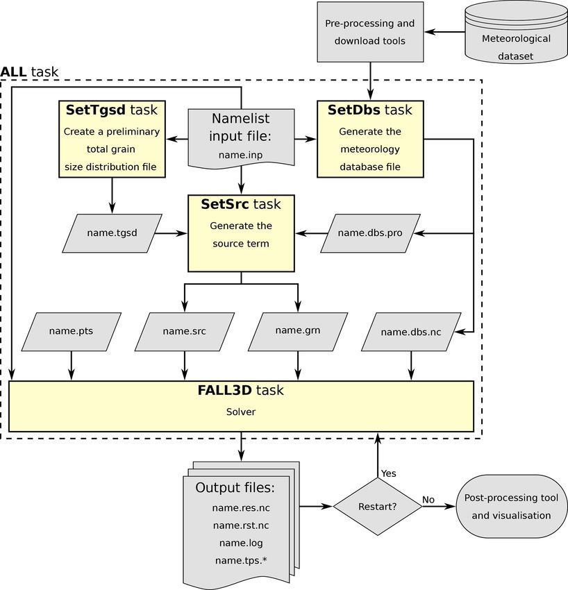
– Parallel model I/O using NetCDF and parallel model the ground deposition flux (ud is the ground deposition ve-
pre-process. In addition, all the pre-process auxiliary locity). Note that when the deposition flux D coincides with
programmes have been embedded within the main code the sedimentation flux G (i.e. when us = ud ), the boundary
(a single multipurpose executable exists in v8.0). The condition at ground reduces to the standard free-flow condi-
code can now be run to perform different tasks indi- tion imposed at 0N .
vidually or sequentially through a single parallel work- Equation (1) is the so-called ADS equation and, in
flow. As a result, all the pre-process, modelling and FALL3D-8.0, has been extended to handle other substances
post-process workflows can now run as a single exe- different from tephra. Note that the passive transport equa-
cution concatenating all tasks and without needing to tion (Eq. 1) neglects inertial terms and, consequently, as-
write/read intermediate files to/from disk. In large prob- sumes a low (≤ 1) particle Stokes number. In a general sense,
lems, this saves substantial disk space and I/O time be- substances in FALL3D-8.0 are grouped in three broad cat-
cause the required model input data (e.g. interpolated egories: particles, aerosols and radionuclides. The category
meteorological fields) are already stored in each proces- “particles” includes any inert substance characterised by a
sor memory when running the FALL3D model task. sedimentation velocity. In the context of FALL3D-8.0, the
category “aerosol” refers to substances potentially non-inert
– A hierarchy of MPI communicators has been defined. (i.e. with chemical or phase changes mechanisms) and hav-
This is actually not active yet in v8.0 but gives flexibil- ing a negligible sedimentation velocity. Finally, the category
ity to extend some code functionalities in a near future “radionuclides” refers to isotope particles subject to radioac-
with little refactoring effort. For example, plans for fu- tive decay. Each of these categories admits, in turn, different
ture versions include ensemble modelling using the Par- subcategories or “species”, defined internally as structures of
allel Data Assimilation Framework (PDAF) or model data that inherit the parent category properties (see Table 3).
nesting. These will require of teams of processors asso- For example, particles can be subdivided into tephra or min-
ciated with different ensemble members or model grids, eral dust; aerosol species can include H2 O, SO2 , etc.; and ra-
respectively. dionuclides can include several isotope species. Finally, each
www.geosci-model-dev.net/13/1431/2020/ Geosci. Model Dev., 13, 1431–1458, 2020
1434                                                                                               A. Folch et al.: FALL3D-8.0 – Part 1

                                                                           Table 1. Continued.
Table 1. List of Latin symbols. Bold and doubled-lined fonts indi-
cate vector and tensor quantities, respectively.                            Symbol    Units           Definition
                                                                            R         m               radius of gravity current
 Symbol    Units        Definition                                          Re        m               radius of the Earth
 As        –            Suzuki parameter (controls the vertical loca-       ra        s m−1           aerodynamic resistance
                        tion of the maximum of the emission)                rb        s m−1           quasi-laminar resistance
 C         kg m−3       scaled concentration (c)                            Re        –               Reynolds number
 Ca        J kg−1 K−1   air specific heat capacity at constant pressure     Ri        –               Richardson number
 Cd        –            particle drag coefficient                           Rib       –               Richardson bulk number
 Cs        J kg−1 K−1   solid (particles) specific heat capacity at con-    S         kg m−3 s−1      mass source term per unit time and volume
                        stant pressure                                      Sc        –               Schmidt number
 Cv        J kg−1 K−1   gas specific heat capacity at constant pressure     St        –               Stokes number of particles
 c         kg m−3       mass concentration of a substance mixed             t         s               time
                        within a fluid (air)                                t1/2      s               radioactive element half live
 D         kg m−2 s−1   ground deposition mass flux (D = c ud )             Ta        K               air temperature
 Df        –            fractal exponent                                    To        K               magma (mixture) temperature at the vent
 d         m            particle sphere equivalent diameter                 U         m s−1           scaled velocity U = (U, V , W )
 dA        m            diameter of particle aggregates                     u         m s−1           fluid velocity vector (wind velocity)
 dn        m            average between particle minimum (d3 ) and                                    u = (u, v, w)
                        the maximum (d1 ) dimensions                        ud        m s−1           ground deposition velocity vector
 ds        m            equivalent diameter of saltating particles          us        m s−1           settling (terminal) velocity vector
 F         kg m−2 s−1   advective mass flux (F = c u)                                                 us = (0, 0, −ws )
 FV        kg m−2 s−1   vertical resuspension emission flux                 uh        m s−1           horizontal wind velocity modulus
 FH        kg m−2 s−1   horizontal flux of saltating particles              ur        m s−1           radial velocity
 fi        –            mass fraction of the ith bin                        u∗        m s−1           friction velocity
 G         kg m−2 s−1   sedimentation mass flux (G = c us )                 u∗t       m s−1           threshold friction velocity
 Gh        –            stability function (see Eq. 18)                     V         m3              volume (of a computational grid cell)
 Gm        –            stability function (see Eq. 17)                     X         m               scaled coordinates X = (X1 , X2 , X3 )
 g         m s−2        gravity acceleration modulus                        z         m               vertical coordinate; distance from the ground
 H         kg m−2 s−1   diffusive mass flux (H = −K∇c)                      zb        m               top bottom height (above terrain)
 H         m            eruption column height                              zo        m               ground roughness height
 HT        m            top of the computational domain                     zt        m               emission top height (above terrain)
 h         m            terrain height (topography)
 hc        m            cloud thickness
 hp        m            height of the atmospheric boundary layer
                        (ABL)
                                                                           subcategory of species is tagged with an attribute name that
 I         kg m−3 s−1   mass sink term per unit time and volume            is used for descriptive purposes only.
 K         m2 s−1       diffusion tensor                                      Depending on the species under consideration, the mass
 kf        –            fractal pre-factor                                 source S and sink I terms in Eq. (1) can be decomposed as
 kh        m2 s−1       horizontal component of the diffusion tensor
 kht       m2 s−1       horizontal diffusion by transport (see Eq. 7)      S =S e + S a + S r + S c
 khn       m2 s−1       horizontal numerical diffusion (see Eq. 8)
 kr        s−1          isotope decay rate
                                                                           I =I w + I a + I r + I c ,                                             (3)
 kv        m2 s−1       vertical component of the diffusion tensor
 L         m            Monin–Obukhov length                               where the superscripts denote emission source terms (S e ; see
 lc        m            characteristic length scale                        Sect. 3.2.3), wet deposition sinks (I w ; see Sect. 3.2.4), parti-
 M         –            Jacobian transformation matrix (components         cle aggregation source and sinks (S a and I a , respectively; see
                        mij )                                              Sect. 3.2.6), radioactive decay source and sinks (S r and I r ,
 Mip       kg s−1       emission rate for bin i at source point p
                                                                           respectively; see Sect. 3.2.7), and chemical reactions’ source
 Mo        kg s−1       total emission rate (source strength)
 mi        –            mapping factors (m1 , m2 , m3 ) (diagonal          and sinks (S c and I c ). Note that FALL3D-8.0 does not ac-
                        terms of Jacobian matrix)                          count for aerosol chemistry yet. However, the code has been
 n         –            outwards unit normal vector                        designed to allow incorporating this functionality in future
 N         s−1          Brunt–Väisälä frequency                            versions in a straightforward manner.
 nb        –            number of species discrete bins
 no        –            gas mass fraction
                                                                              When the ADS equation (Eq. 1) is discretised, species in
 np        –            number of point sources in emission schemes        the mixture are binned in nb discrete “classes” or bins, so that
           m−3 s−1                                                         the total concentration c at any point of the domain
 ṅtot                  total particle decay per unit volume and time
                                                                                                                               Pnb decom-
 Prt       –            turbulent Prandtl number                           poses as the sum of bin concentrations, i.e. c = i=1      ci . Sub-
 pmn       –            relative probability of decay of the isotope m
                                                                           stitution of bin discretisation in Eq. (1) yields to nb equations
                        to the isotope n
 q         m3 s−1       volumetric flow rate into the plume umbrella       (one per discrete bin), each formally identical to Eq. (1):
                        region
                                                                           ∂ci
                                                                               + ∇ · F i + ∇ · Gi + ∇ · H i = Si − Ii i = 1 : nb .                (4)
                                                                           ∂t

Geosci. Model Dev., 13, 1431–1458, 2020                                                       www.geosci-model-dev.net/13/1431/2020/
A. Folch et al.: FALL3D-8.0 – Part 1                                                                                                                            1435

Table 2. List of Greek symbols.

        Symbol      Units          Definition
        α           –              constant of Smagorinsky
        αe          –              radial plume entrainment coefficients
        αs          m s−2          sandblasting efficiency coefficient
        βe          –              cross-wind plume entrainment coefficients
        ϕ           –              particle aspect ratio (see Eq. 22)
        φ           Rad            latitude
        φ           –              flux limiter function
        φh          –              atmospheric stability function for temperature
        1g          m              characteristic grid cell measure
        1t          s              time increment (step)
        0           –              boundary of the computational domain (divided in Dirichlet 0D , Neumann 0N and Robin 0R parts)
        γ           Rad            colatitude
        γ           s−1            mean shear rate of wind
        3           s−1            wet deposition scavenging coefficient
        λ           Rad            longitude
        λs          –              Suzuki parameter (controls the distribution of the emitted mass around the maximum)
        λc          m              asymptotic length scale (λc = 30 m assumed)
        λg          –              empirical constant in plume gravity currents (λg = 0.2 assumed)
        κ           –              von Karman constant (κ = 0.4 assumed)
        9           –              particle sphericity
        ρa          kg m−3         fluid (air) density
        ρp          kg m−3         particle density
        θ           K              potential temperature
        θ∗          K              potential temperature scale
        θv          K              potential virtual temperature
        νa          Pa s           fluid (air) kinematic viscosity
        ξ           –              particle shape factor (sphericity to circularity ratio)

Table 3. Types of categories and related subcategories of species in FALL3D-8.0.

                   Category               Subcategory          Name              Bins                  Comments
                                          (species)            (tag)             (number)
                                                               lapilli           user defined1         tephra with 82 < −1
                                          tephra               coarse ash        user defined          tephra with −1 ≤ 8 ≤ 4
                   Particles
                                                               fine ash          user defined          tephra with 8 > 4
                                                               aggregate         one or more           aggregation model dependent
                                          mineral dust         dust              user defined1
                                          H2 O                 H2O               1                     water vapour
                   Aerosols
                                          SO2                  SO2               1                     sulfur dioxide only3
                                          134 Cs               CS-134            user defined1         cesium-134, decays to a stable isotope
                                          137 Cs               CS-137            user defined          cesium-137, decays to a stable isotope
                   Radionuclides          131 I                I-131             user defined          iodine-131, decays to a stable isotope
                                          90 Sr                SR-90             user defined          strontium-90, decays to yttrium 90
                                          90 Y                 Y-90              user defined          yttrium-90, decays to a stable isotope
                 1 For any species in the category particles or radionuclides, users can specify the number of effective bins from a grain size distribution.
                 2 For tephra, the 8 number is defined as d = 2−8 , where d is the particle diameter in millimetres. 3 SO chemistry not included yet in
                                                                                                                           2
                 v8.0.

www.geosci-model-dev.net/13/1431/2020/                                                                              Geosci. Model Dev., 13, 1431–1458, 2020
1436 A. Folch et al.: FALL3D-8.0 – Part 1
Table 4. Parameterisations available in FALL3D-8.0 depending on each category and related subcategory (species). Note that, except for
radioactive decay, all physical phenomena were already included in v7.x. However, several parameterisations have been updated to account
for more recent developments.
Category Particles Aerosols Radionuclides
Subcategory (species) tephra dust (all species) (all species)
√ √ √ √
Diffusion (Sect. 3.2.1)
√ √ √
Particle sedimentation (Sect. 3.2.2)
√ √ √
POINT
√ √ √
HAT
√ √1 √
Emissions (Sect. 3.2.3) SUZUKI
√ √1
PLUME
√ √
RESUSPENSION
√ √ √ √
dry deposition 2
Deposition mechanisms (Sect. 3.2.4) √ √ √ √
wet deposition 3
√ √1
Gravity current (Sect. 3.2.5)
√
Aggregation (Sect. 3.2.6)
√
Radioactive decay (Sect. 3.2.7)
√(4)
Chemical reactions
1 Only for volcanic aerosols. 2 Applies only to particles/aerosols smaller than 100 µm. 3 Cut-off at 100 and 1 µm assumed for below- and
in-cloud scavenging, respectively. 4 Not included yet in v8.0.
Note that the nb equations for bins can be coupled by In the case of FALL3D-8.0, the horizontal coefficient kh can
means of the source and sink terms, which define the even- be either assumed constant or parameterised as in Byun and
tual transfer of mass among different bins, e.g. in the case Schere (2006):
of particle aggregation/disegregation, chemical reactions and
formation of child radionuclides. 1 1 1
= + , (6)
kh kht khn
3.2 Model parameterisations
where
Parameterisations in FALL3D have been revised and up- q
dated, removing deprecated options and adding new options kht = 2 α 2 12g S02 + S3
2
available from more recent studies. Table 4 shows the param-
s
∂u ∂v 2 ∂u ∂v 2
eterisations implemented in FALL3D-8.0 that are described 2 2
= α 1g − + + (7)
in the following subsections. ∂x ∂y ∂x ∂y
3.2.1 Diffusion tensor
1ref
khn = kref . (8)
The atmospheric flow is characterised by large horizontal- 1g
to-vertical aspect ratios of wind velocities and length scales,
as well as by an anisotropic momentum diffusion with the In the equations above, 1g is a characteristic grid cell mea-
horizontal diffusion coefficient being typically much larger sure (e.g. the equivalent area length), α ∼
= 0.28 denotes the
than the vertical one (e.g. Schaefer-Rolffs and Becker, 2013). Smagorinsky constant, S0 and S3 are the stretching and
For this reason, model diffusion that accounts for subgrid- shear strength (i.e. the two components of the bi-dimensional
scale atmospheric eddies is typically assumed anisotropic, wind deformation), and kref is a reference horizontal diffu-
with two distinct eddy diffusion coefficients along the hor- sion for a reference grid cell size 1ref (FALL3D-8.0 con-
izontal and vertical dimensions: siders kref = 8000 m2 s−1 for 1ref = 4 km). Equation (6) was
proposed by Byun and Schere (2006) to overcome the de-
kh 0 0 pendency of horizontal diffusion on grid resolution and com-
K = 0 kh 0 . (5) bines a Smagorinsky subgrid-scale (SGS) model giving the
0 0 kv diffusion by transport (kht ) with a formula that counteracts
Geosci. Model Dev., 13, 1431–1458, 2020 www.geosci-model-dev.net/13/1431/2020/A. Folch et al.: FALL3D-8.0 – Part 1 1437
numerical over-diffusion in coarse discretisations (khn ) so 1979; Jacobson, 1999)
that the smaller one between kht and khn dominates. In this g [θv (zr ) − θv (zo )] (zr − zo )
way, the effect of the transportive diffusion is minimised for Rib = , (14)
coarse grids, whereas for fine discretisations the numerical θ v uh (zr )2
diffusion term is reduced. where zr and zo denote the reference and the ground rough-
The vertical diffusion coefficient kv can also be either as- ness heights, and θ v denotes the average between the two
sumed constant or parameterised according to the similarity vertical levels. Given Rib , one can estimate u∗ and θ∗ as
theory and distinguishing among surface layer, atmospheric κuh (zr ) p
boundary layer (ABL) and free atmosphere (e.g. Neale et al., u∗ ≈ Gm (Rib ) (15)
ln(zr /zo )
2010):
κzu∗
φh
for z
hp κ 2 uh [θv (zr ) − θv (zo )] p
κzu∗ z 2
θ∗ ≈ Gh (Rib ), (16)
kv = φh 1 − h for z < hp (9) u∗ Prt ln2 (zr /zo )
l 2 ∂uh Fc (Ri) for z > hp ,
c ∂z where Prt is the turbulent Prandtl number (Prt ≈ 1) and the
stability functions Gm and Gh are given by (Louis, 1979;
where κ is the von Karman constant (κ = 0.4), z is the dis- Jacobson, 1999)
tance from the ground, u∗ is wind friction velocity, φh is
9.4Rib
the atmospheric stability function for temperature, hp is the 1 − Rib ≤ 0
1+70κ 2 (|Rib |zr /zo )0.5 /ln2 (zr /zo )
ABL height, lc is a characteristic length scale, uh is the hor- Gm = (17)
1
izontal wind velocity modulus, and Fc is a stability func-
(1+4.7Ri )2 Rib > 0
b
tion which depends on the Richardson number Ri. For lc and
Fc , FALL3D-8.0 adopts the relationships used by the Com-
1 − 9.4Rib
Rib ≤ 0
munity Atmosphere Model (CAM) 4.0 model (Neale et al., 1+50κ 2 (|Rib |zr /zo )0.5 /ln2 (zr /zo )
Gh = (18)
2010): 1
Rib > 0.
(1+4.7Rib )2
1 −1
1 3.2.2 Sedimentation velocity
lc = + (10)
κz λc
Particle bins in the model are assumed to settle down with a
( sedimentation velocity us = (0, 0, −ws ) equal to its terminal
1
1+10Ri(1+8Ri) stable (Ri > 0) velocity:
Fc (Ri) = √ (11)
1 − 18Ri unstable (Ri < 0), s
4g (ρp − ρa ) d
where λc is the so-called asymptotic length scale (λc ≈ ws = , (19)
3 Cd ρa
30 m). The atmospheric stability function for temperature φh
is calculated as where ρa and ρp denote air and particle density, d is the par-
ticle equivalent diameter, and Cd is the drag coefficient that
βh + Lz z/L > 1 stable atmosphere depends on the Reynolds number, Re = dus /νa (νa = µa /ρa
being the kinematic viscosity of air and µa its dynamic vis-
φh = 1 + βh Lz 0 ≤ z/L ≤ 1 nearly neutral cosity). For irregular particles, the drag coefficient Cd has to
be obtained from experimental measurements. FALL3D-8.0
1 − γh z
−1/2
z/L < 0 unstable atmosphere,
L includes several parameterisations derived from laboratory
(12) results using natural and synthetic particles and that cover
a wide range of particle sizes and shapes (characterised by
where βh = 5, γh = 15, and L is the Monin–Obukhov length, sphericity, by circularity, or by some other model shape fac-
defined as tor). Model options for the drag coefficient Cd include the
following:
u2∗ θ v
L= , (13)
κgθ∗ 1. The GANSER model (Ganser, 1993) shows that
24 n o
with g denoting gravity, θ v the mean potential virtual tem- Cd = 1 + 0.1118(Re K1 K2 )0.6567 (20)
perature and θ∗ the potential temperature scale. The param- ReK1
eters in Eq. (13) (i.e. L or u∗ /θ∗ ) are ideally furnished by 0.4305K2
+ 3305
,
the driving meteorological model. If not, and alternatively, 1 + ReK K
1 2
FALL3D-8.0 estimates the friction velocity u∗ and the po-
tential temperature scale θ∗ from the potential virtual tem- where K1 = 3/[(dn /d) + 29 −0.5 ] and K2 =
1.8148(−Log9)0.5743
perature θv and the Richardson bulk number Rib as (Louis, 10 are two shape factors, dn is
www.geosci-model-dev.net/13/1431/2020/ Geosci. Model Dev., 13, 1431–1458, 20201438 A. Folch et al.: FALL3D-8.0 – Part 1
the average between the minimum and the maximum a data structure made of np discrete points, each “tagged”
axis, and 9 is the particle sphericity (9 = 1 for with a time-varying position and bin emission rate (source
spheres). For calculating the sphericity, it is practical strength) Mip (in kg s−1 ). As a result, Sie in a model grid cell
to use the concepts of “operational” and “working results from summing emissions from all point sources lay-
sphericity”, 9work introduced by Wadell (1933) and ing within the cell volume V :
Aschenbrenner (1956), which are based on the deter-
np
mination of the volume and of the three dimensions of X
Sie = Mip /V . (24)
a particle, respectively:
p=1
(P 2 Q)1/3 The total source strength Mo results from summing over all
9work = 12.8 p ,
1 + P (1 + Q) + 6 1 + P 2 (1 + Q2 ) source points and bins, i.e.
(21) np
nb X nb
X X
Mo = Mip = Mi . (25)
with P = d3 /d2 , Q = d2 /d1 , where d1 is the longest
i=1 p=1 i=1
particle dimension, d2 is the longest dimension perpen-
dicular to d1 , and d3 is the dimension perpendicular to
Table 5 summarises the different (exclusive) options avail-
both d1 and d2 .
able in FALL3D-8.0 for the emission term and related source
2. The PFEIFFER model (Pfeiffer et al., 2005), based on strength.
the interpolation of previous relationships by Walker
1. The POINT option assumes that all mass is emitted from
et al. (1971) and Wilson and Huang (1979), shows
a single point (np = 1) located at height zt above ground
24 −0.828 √ level:
Re ϕ
+2 1−ϕ Re ≤ 102 (
Cd = 1 − 1−Cd |Re=102 (103 − Re) 102 ≤ Re ≤ 103 fi Mo z = zt
900 Mi1 = (26)
Re ≥ 103 , 0 z 6 = zt ,
1
(22)
where fi is the ith bin mass fraction.
where ϕ = (b + c)/2a is the particle aspect ratio (a ≥ 2. The HAT option defines a uniform vertical line of np
b ≥ c denote the particle semi-axes). source points spanning in height from zb (bottom) to zt
3. The DIOGUARDI model (Dioguardi et al., 2018) (top) above the ground (i.e. with thickness zt − zb ):
demonstrates that (f M
i o
np zb ≤ z ≤ zt
0.25 Mip = (27)
24 1 − ξ 0 otherwise.
Cd = +1
Re Re
24 0.08 0.4251 Note that this option includes as end-members the
+ (0.1806Re0.6459 )ξ −Re , POINT option (if zb = zt ) and a vertically uniform emis-
Re 1 + 6880.95
2 ξ
5.05
Re sion from ground to top (if zb = 0).
(23)
3. The SUZUKI option (Suzuki, 1983; Pfeiffer et al., 2005)
where ξ is a particle shape factor (sphericity to circular- assumes a mushroom-like vertical distribution of np
ity ratio), for which Dioguardi et al. (2018) suggested an emission points depending on two dimensionless pa-
empirical correlation with sphericity 9 as ξ = 0.839. rameters (As and λs ):
Note that, in any case, the terminal velocity ws is defined z λs
fi M o z A −1
by a triplet (d, ρp , 9). As a result, particles with similar val- Mip = 1− e s zt 0 ≤ z ≤ zt . (28)
ues of the three parameters can be grouped within the same np zt
model bin.
The Suzuki parameter As controls the vertical location
3.2.3 Emissions of the maximum of the emission profile, whereas the
parameter λs controls the distribution of the emitted
The emission source term for the ith bin (Sie term in the bin mass around the maximum. When any of the previous
equations; see Eq. 4) gives the mass per unit of time and vol- source options are defined for volcanic plumes, it is use-
ume (units of kg m−3 s−1 ) released at each point (cell) of the ful to prescribe the total source strength (eruption mass
computational domain. FALL3D-8.0 can generate and han- flow rate) Mo in terms of the eruption column height
dle multiple types of emission sources, internally defined as H because this parameter is easier to be obtained from
Geosci. Model Dev., 13, 1431–1458, 2020 www.geosci-model-dev.net/13/1431/2020/A. Folch et al.: FALL3D-8.0 – Part 1 1439
Table 5. Options available in FALL3D-8.0 for vertical distribution of mass and total source strength depending on the type of emission
source S e .
Type of source Vertical distribution of mass Total source strength Mo options Comments
POINT Prescribed (same for all bins) (i) Prescribed; (ii) given by Vertical distributions valid for any
HAT Eq. (29); (iii) given by Eq. (30) type of bin but source strength op-
SUZUKI tions (ii) and (iii) are for volcanic
particles only
PLUME Computed by the FPLUME-1.0 (i) Prescribed; (ii) computed by Only for volcanic particles/
model (bin dependent) FPLUME-1.0 model from eruption aerosols
column height (inverse problem)
RESUSPENSION Distributed linearly within the ABL Computed from surface cell area Only for resuspended particles
or assigned to the first vertical and vertical flux using emission (ash and dust)
model layer (bin dependent) schemes (Eqs. 33, 34 or 36)
direct observations. To this purpose, FALL3D-8.0 in- 1-D cross-section-averaged eruption column model
cludes two relationships that correlate Mo with H based based on the buoyant plume theory (BPT). The model
on empirical observations and on 1-D plume model sim- accounts for plume bending by wind, entrainment of
ulations, respectively. The first and simplest case con- ambient moisture, effects of water phase changes, parti-
siders the fit proposed by Mastin et al. (2009): cle fallout and re-entrainment, and a model for wet ag-
gregation of ash particles in the presence of liquid water
Mo = aH 4.15 , (29) or ice. As opposed to the previous cases, the PLUME
where a = 140.8 is a constant and H is the eruption source option automatically determines a bin-dependent
column height expressed in kilometres above the erup- vertical distribution of mass and computes height from
tive vent. Alternatively, the 1-D model fit by Woodhouse Mo , or vice versa by solving an inverse problem.
et al. (2016) can also be used to provide Mo depending
on the surrounding atmospheric conditions:
5. The RESUSPENSION option considers the remobilisa-
Mo = co N 3 H 4 f (W ), (30) tion and resuspension by wind of soil particles (e.g.
where N is the Brunt–Väisälä frequency, co is a con- mineral dust or volcanic ash previously deposited on
stant, and f is a function of the parameter W = the ground). Up to three different emission schemes are
1.44γ /N given by available in FALL3D-8.0 to obtain the vertical flux of
suspended particles, from which Mo is obtained by mul-
2 4
!
1 + bW + cW tiplying by the associated surface cell area (see Folch
f (W ) = , (31) et al., 2014, for details). Typically, the emission schemes
1 + aW
for mineral dust are formulated in terms of the fric-
with the coefficients a = 0.87 + 0.05βe /αe , b = 1.09 + tion velocity. For example, emission scheme 1 (West-
0.32βe /αe , and c = 0.06+0.03βe /αe , with αe and βe the phal et al., 1987) considers
radial and cross-wind plume entrainment coefficients
(Costa et al., 2016b) and γ the mean shear rate of wind. (
0 u∗ < u∗t
The constant co in Eq. (30) depends on the conditions at FV = (33)
the vent: 10−5 u4∗ u∗ ≥ u∗t ,
0.35 αe2 ρa Ca Ta
co = , (32)
g [(Cv no + Cs (1 − no ))To − Ca Ta ] where FV is the vertical flux (in kg m−2 s−1 ), occurring
with Cs , Cv and Ca the specific heat capacities at con- only above a (constant) threshold friction velocity u∗t
stant pressure of the solid pyroclasts, gas phase and air, (u∗ given in m s−1 ). An important limitation of Eq. (33)
respectively, Ta and To the air and vent magma mixture is that the vertical flux does not depend on either parti-
temperatures, and n0 the gas mass fraction. cle size or soil moisture. However, despite its simplic-
ity, this parameterisation can be useful when informa-
4. The PLUME option, valid only for volcanic plumes, tion on soil characteristics (e.g. particle sizes and densi-
uses the FPLUME-1.0 model (Folch et al., 2016) em- ties, moisture, roughness) is unavailable or poorly con-
bedded in FALL3D-8.0. FPLUME-1.0 is a steady-state strained. Emission scheme 2 (Marticorena and Berga-
www.geosci-model-dev.net/13/1431/2020/ Geosci. Model Dev., 13, 1431–1458, 20201440 A. Folch et al.: FALL3D-8.0 – Part 1
metti, 1995; Marticorena et al., 1997) considers 3.2.4 Deposition mechanisms
0
u∗ < u∗t In FALL3D-8.0, dry and wet deposition mechanisms can be
FV = ρa 3
2
u∗t
u∗t
activated for any type of bin below a certain particle/aerosol
Sc u∗ 1 − 2
1+ u∗ ≥ u∗t , size.
g u∗ u∗
Dry deposition on the ground is imposed prescribing the
(34)
deposition velocity through a Robin boundary condition in
where the experimental coefficient Sc (in cm−1 ) de- Eq. (2). FALL3D-8.0 admits two dry deposition parame-
pends on the amount of available fine particles in the terisations which describe the vertical depositional fluxes
soil, and the threshold friction velocity is given by by Brownian diffusion and inertial impaction, parameterised
through the Schmidt and the Stokes numbers, respectively.
u∗t = The first option considers the mass-consistent formulation
proposed by Venkatram and Pleim (1999):
(
0.129 K
(1.928Re0.092 −1)0.5
0.03 < Re ≤ 10
0.129K(1 − 0.0858e−0.0617(Re−10) ) Re > 10, ws 1
|ud | = ws + ≈ ws + , (39)
(35) 1 − e a +rb )ws
−(r ra + rb
r
where ra describes the effects of aerodynamic resistance and
ρp gd
with K = ρa 1 + ρ0.006
gd 2.5 and Re = 1331 × d 1.56
p rb the quasi-laminar resistance (e.g. Brandt et al., 2002, and
(the lower bound of the fit corresponds to particles of references therein). The aerodynamic resistance ra can be
≈ 10 µm in size). Note that in Eq. (35), ρp and ρa are calculated as
particle and air densities (expressed in g cm−3 ), g is z
gravity (in cm s−2 ), d is the particle size (in centime- 1 z
ra = ln − φh , (40)
tres), Re is the Reynolds number parameterised as a ku∗ zo L
function of the particle size, and u∗t is given in cm s−1 .
with zo denoting the ground roughness height and φh the
Finally, emission scheme 3 (Shao et al., 1993; Shao and atmospheric stability function for temperature given by
Leslie, 1997; Shao and Lu, 2000) considers that the up- Eq. (12). The quasi-laminar resistance rb can be expressed
lift from surface of the fine fraction of soil particles is in terms of the Schmidt number Sc = ν/D and Stokes num-
controlled by the bombardment of saltating particles of ber St = ws u2∗ /(gν) (with ν kinematic viscosity of air and D
larger sizes (≥ 63 µm), which breaks the cohesive forces molecular diffusivity of particles) (e.g. Brandt et al., 2002):
of smaller particles.
Based on theoretical and experimental results, Shao 1
rb = . (41)
et al. (1993) found an expression for the vertical flux of u∗ Sc−2/3 + 10−3/St
dust particles of size d ejected by the impact of saltating
particles of size ds : The second option is that proposed by Feng (2008), which
essentially differs from Eq. (39) in the estimation of rb :
αs (d, ds )
FV (d, ds ) = FH (ds ), (36)
u2∗t (d) 1
|ud | = ws + ∗ 2
, (42)
where αs (in m s−2 ) is the coefficient of sandblasting ra + 1/(u∗ c1 e−0.5[(Re −c2 )/c3 ] + aub∗ )
efficiency determined experimentally (Shao and Leslie,
where c1 = 0.0226, c2 = 40300 and c3 = 15330 are dimen-
1997) and FH is the horizontal flux (in kg m−1 s−1 ) of
sionless parameterisation constants, Re∗ is the Reynolds
saltating particles:
number (computed with the friction velocity u∗ ), and a and
0 u∗ < u∗t (ds ) b are coefficients that depend on the particle size and surface
FH (ds ) = ρ u 3
u2 (d ) (37) characteristics. Note that Feng (2008) gives a and b best-
co a ∗ 1 − ∗t 2 s u∗ ≥ u∗t (ds ),
g u ∗ fit values for seven land use categories and four aerosol size
where co is an empirical dimensionless constant close to modes: nuclei (up to 0.1 µm), accumulation (up to 2.5 µm),
1. In this scheme, the threshold friction velocity u∗t (d) coarse (up to 10 µm) and giant (up to 100 µm). A cut-off is
is given by assumed above this size because the sedimentation velocity
s term ws dominates, and therefore the dry deposition contri-
bution can be neglected.
ρp gd γ
u∗ts = 0.0123 + , (38) Wet deposition mechanisms in FALL3D-8.0 are assumed
ρa ρa d
to occur only within the ABL, and the corresponding sink
where γ is an experimental parameter ranging between term in Eq. (3) is parameterised as
1.65×10⁻⁴ and 5×10⁻⁴ kg s2 (a value of 3×10⁻⁴ kg s2
is assumed in FALL3D-8.0). I w = 3 c, (43)
Geosci. Model Dev., 13, 1431–1458, 2020 www.geosci-model-dev.net/13/1431/2020/A. Folch et al.: FALL3D-8.0 – Part 1 1441
where 3 differs for in-cloud (ic) and below-cloud (bc) sinks. Given the radius R, the radial velocity field as a function of
For below-cloud scavenging (precipitation), 3bc is estimated distance r is calculated as (Costa et al., 2013)
from the total precipitation rate as (e.g. Brandt et al., 2002;
1 r2
Jung and Shao, 2006) 3 R
ur (r) = ur (R) 1+ (0 ≤ r ≤ R), (49)
4 r 3 R2
3bc = a P b , (44)
where ur (R) is the front velocity:
where P is the precipitation rate (in mm h−1 ),
and a = 8.4 ×
2λg N q 1/2 1
10−5 and b = 0.79 are two empirical constants. For in-cloud ur (R) = √ . (50)
scavenging (rainout), the model considers a parameterisation 3π R
based on the atmospheric relative humidity (RH; in %) as in In order to avoid sudden jumps at the gravity current front,
Brandt et al. (2002): FALL3D-8.0 interpolates the front velocity ur (R) with far
field wind velocity using an exponential decay function of
0 for RH < RHt
3ic = RH−RHt (45) the cloud thickness hc as
ARH RH s −RHt
for RH ≥ RHt ,
exp[−r/(4hc )], (51)
with ARH = 3.5 × 10⁻⁵ , RHt = 80 % (threshold value) and
RHs = 100 % (saturation value). Two critical particle cut-off where r is the distance from the current front.
sizes of 100 and 1 µm are assumed for below- and in-cloud
3.2.6 Aggregation
scavenging, respectively.
Aggregation of tephra particles can occur inside the erup-
3.2.5 Gravity spreading of the umbrella region
tive columns or even downwind in ash clouds during atmo-
Large explosive volcanic eruptions can generate gravity- spheric dispersion, thereby affecting the sedimentation dy-
driven transport mechanisms that dominate over passive namics and deposition of volcanic ash. FALL3D-8.0 includes
transport close to the vent and cause a radial spreading of some simple a priori aggregation options and a wet aggrega-
the cloud (e.g. Woods and Kienle, 1994; Sparks et al., 1997). tion model (Costa et al., 2010; Folch et al., 2010) that can
In order to simulate this mechanism, FALL3D-8.0 includes be activated for tephra bins. The a priori options consist of
a gravity current model (see Costa et al., 2013, and the erra- user-defined or empirically based predefined fractions of ag-
tum published in June 2019). This option consists on adding gregating classes being transferred to one or more class of
a radial velocity field to the background wind, so that con- aggregates at the source points (i.e. aggregation is performed
tributions from both passive and density-driven mechanisms before transport). In contrast, in the wet aggregation model,
are accounted for. The added radial wind is centred above ash particles aggregate on a single effective class of diame-
the eruptive vent in the umbrella region and extended up to a ter dA ; i.e. aggregation only affects tephra bins with diameter
radius R given by smaller than dA , typically in the range 100–300 µm. This op-
tion can run embedded in FPLUME-1.0 or as a stand-alone
1/3 module. Consider a tephra grain size distribution in which
3λg N q
R= t 2/3 , (46) k particle bins can aggregate. Then, the aggregation model
2π
defines the source (S a ) and sink (I a ) bin terms for the corre-
where t is time since eruption onset, λg is an empirical con- sponding k + 1 bins as
stant constrained to ≈ 0.2 from direct numerical simulations (
a = kj =1 Ija
P
(Suzuki and Koyaguchi, 2009), N is the Brunt–Väisälä fre- Sk+1
πd ρ (52)
quency, and q is the volumetric flow rate into the umbrella Ija = 6j j ṅj j = 1 : k,
region, estimated as (Morton et al., 1956; Suzuki and Koy-
aguchi, 2009; Costa et al., 2013, as correct in the erratum where dj (< dA ) and ρj are, respectively, the diameter and
published in 2019) density of particles in bin j , and ṅj is the number of particles
per unit volume and time that aggregate. The model assumes
1/2 3/4 that this is proportional to the total particle decay per unit
c ke Mo
q= , (47) volume and time ṅtot , i.e.
N 5/4
where Mo is the total source strength (i.e. mass eruption rate), Nj
ṅj ≈ Pk ṅtot , (53)
ke is the air entrainment coefficient, and c is a constant that i=1 Ni
from varies from tropical to midlatitude/polar locations:
where
(
0.43 m3 kg−3/4 s−3/2 for tropical
dA
df
c= (48) Nj = kf (54)
0.87 m3 kg−3/4 s−3/2 midlatitude/polar. dj
www.geosci-model-dev.net/13/1431/2020/ Geosci. Model Dev., 13, 1431–1458, 20201442 A. Folch et al.: FALL3D-8.0 – Part 1
Table 6. List of radionuclides implemented in the model. Table shows half life, decay rate (in s−1 ) and resulting child product.
Radionuclide t1/2 t1/2 (s) kr (s−1 ) Product
134 Cs 2.065 years 6.51 × 10⁷ 1.06 × 10⁻⁸ 134 Ba (stable)
137 Cs 30.17 years 9.51 × 10⁸ 7.29 × 10⁻¹⁰ 137 Ba (stable)
131 I 8.0197 days 6.93 × 10⁵ 1.00 × 10⁻⁶ 131 Xe (stable)
90 Sr 28.79 years 9.08 × 10⁸ 7.63 × 10⁻¹⁰ 90 Y (unstable)
90 Y 2.69 days 2.33 × 10⁵ 2.98 × 10⁻⁶ 90 Zr (stable)
is the number of primary particles of diameter dj in an ag- and decays to the stable isotope 90 Zr. The production rate Snr
gregate of diameter dA , kf is a fractal pre-factor (kf ≈ 1), and of 90 Y is therefore equivalent to the decay rate of 90 Sr.
Df is the fractal exponent (Df ≤ 3). The model estimates the In FALL3D-8.0, the radioactive decay is implemented by
total particle decay per unit time ṅtot integrating the coagu- firstly transporting the radionuclides for a time step 1t and
lation kernel over all particle sizes, depending on the stick- then by evaluating the decay during the same time step. For
ing efficiency times a collision frequency function which ac- radionuclides that decay to a stable isotope (134 Cs, 137 Cs and
counts for Brownian motion, collision due to turbulence as 131 I), it is considered that after a time step 1t the concentra-
a result of inertial effects, laminar and turbulent fluid shear, tion decreases as
and differential sedimentation (see Costa et al., 2010; Folch
et al., 2016, for details). c(t + 1t) = c(t) e−kr 1t , (57)
3.2.7 Radioactive decay whereas for decay to an unstable isotope (yttrium), the con-
centration varies as
FALL3D-8.0 can handle the fate of radioactive material dis- h i
persed from accidental releases (e.g. Brandt et al., 2002; cY (t + 1t) = cSr (t)(1 − e−kSr 1t ) + cY (t) e−kY 1t , (58)
Leelössya et al., 2018). Five common species of radionu-
clides have been implemented: cesium (134 Cs, 137 Cs) and io- where cY and cSr are, respectively, the concentrations of 90 Y
dine (131 I), which decay to stable isotopes, and 90 Sr, which and 90 Sr, and kY and kSr are the corresponding decay rates.
decays to the unstable isotope 90 Y (see Table 6).
Radionuclide species need to specify the source (Snr ) and 3.3 Data insertion
the sink (Inr ) terms in Eq. (3) associated with the radioactive
Instrumentation aboard the new generation of geostationary
production or decay of the isotope n, respectively. The ra-
satellites provides an unprecedented level of spatial resolu-
dioactive decay term indicates the mass per unit volume of
tion and temporal frequency (2 to 4 km pixel size and 10
the isotopes of type n that decays per unit time:
to 15 min observation period; see Table 7), yielding a quasi-
Inr = kr cn , (55) global coverage considering the overlap of different existing
platforms. This is very suitable for high-resolution model
where cn is concentration (expressed in kg m−3 ) and kr a con- data assimilation and related uncertainty quantification, as
stant specific of each isotope (decay rate) that can be cal- well as to implement ensemble-based dispersal forecast sys-
culated from the radioactive element half life t1/2 as kr = tems. These aspects are still under development and hope-
ln(2)/t1/2 . Values of t1/2 and kr for common radionuclides fully will be part of next FALL3D model distributions. How-
are reported in Table 6. Note that the decay term is more rel- ever, FALL3D-8.0 already includes the possibility of ini-
evant for isotopes with short half lives, e.g. for 131 I, which tialising a model run from satellite retrievals. This option,
has t1/2 ' 8 d (Brandt et al., 2002; Leelössya et al., 2018). known as data insertion, is typically used in dispersal of vol-
The radioactive decay term of the isotope n constitutes a canic ash and aerosols (mainly SO2 ) in order to reduce model
sink Inr for the isotope itself. However, the decay of the iso- uncertainties coming from the eruption source term.
tope m, father of isotope n, constitutes a source Snr for the Satellite retrievals giving cloud column mass of fine vol-
isotope n: canic ash and aerosols can be furnished to the model to-
Snr = pmn Imr , (56) gether with values of cloud thickness, with the latter needed
in order to compute initial concentration (in kg m−3 ) from
where pmn is the relative probability of decay of the isotope column mass (in kg m−2 ). In the model initialisation step,
m to the isotope n. If the isotope m has only one child n, the gridded satellite data are interpolated into the model grid im-
relative probability of the branch m 7 −→ n is pmn = 1. Note posing conservation of mass when concentration values are
from Table 6 that 134 Cs, 137 Cs and 131 I decay to stable iso- computed for each model grid cell, i.e. ensuring that the re-
topes, whereas 90 Sr decays to 90 Y which, in turn, is unstable sulting column mass in the model (computed concentration
Geosci. Model Dev., 13, 1431–1458, 2020 www.geosci-model-dev.net/13/1431/2020/A. Folch et al.: FALL3D-8.0 – Part 1 1443
Table 7. Characteristics of sensors for ash and SO2 detection aboard the new generation of geostationary satellites. Table courtesy of Andrew
Prata.
Satellite Sensor Coverage Spatial res. (km) Temporal res. (min) Ash/SO2 bands (µm) Lifetime
Meteosat-11 SEVIRI Europe and Africa 3 15 7.35, 8.7, 10.8, 12 2015–2022
FY-4A AGRI S. Asia and Oceania 4 15 8.5, 10.7, 12 2016–2021
Himawari-8 AHI S. Asia and Oceania 2 10 7.35, 8.6, 10.45, 11.2, 12.35 2014–2029
GOES-17 ABI N. America 2 10 7.4, 8.5, 10.3, 11.2, 12.3 2018–2029
GOES-16 ABI S. America 2 10 7.4, 8.5, 10.3, 11.2, 12.3 2016–2027
multiplied by cloud thickness) equals that of satellite data map physical domains (e.g. accounting for Earth’s curvature
over the same cell area. Examples showing how data inser- and topography) to a “brick-like” computational domain (see
tion improves model accuracy are given in the companion Fig. 1) by using coordinate-dependent horizontal and verti-
paper (Prata et al., 2020). cal mappings. On the other hand, a generalised form simpli-
fies the structure and implementation of the code because the
model can be solved on various horizontal (Cartesian, spher-
4 Numerical implementation ical, Mercator, polar stereographic, etc.) and vertical (terrain-
following, σ -coordinate, etc.) coordinate systems using only
4.1 Coordinate mappings and scaling
one solving routine. To this purpose, one needs first to scale
Consider the ADS equation (Eq. 1) written in a Cartesian the model coordinates and some terms in the equation us-
system of coordinates (x, y, z) assuming a diffusion tensor ing adequate mapping and scaling factors, then solve for the
as in Eq. (5) and a sedimentation velocity us = (0, 0, −ws ) scaled concentration C in the regular computational domain
aligned with the vertical coordinate z: c (as in Cartesian coordinates) and, finally, transform the
scaled concentration back to the original one.
∂c ∂(cu) ∂(cv) ∂(cw) ∂(cws ) In general and given two orthogonal coordinate systems,
+ + + −
∂t ∂x ∂y ∂z ∂z (x1 , x2 , x3 ) and (X1 , X2 , X3 ), coordinate mapping factors are
∂
∂c
∂
∂c
∂
∂c
given by the terms mij of the Jacobian transformation matrix
− kh − kh − kv = S − I. (59) M:
∂x ∂x ∂y ∂y ∂z ∂z
∂xi
It is straightforward to discretise the above equation in a mij = , (61)
∂Xj
“brick-like” computational domain c using a structured
regular (i.e. equally spaced) mesh, although the regularity but, for the transformations considered here, M will always
condition is typically relaxed across the vertical direction so be diagonal with three non-zero components (m1 , m2 and
that the vertical grid resolution increases close to ground, m3 ). For example, in the horizontal transformation to spher-
where higher gradients are expected. In order to use other ical Earth surface coordinates (λ, φ), one has
coordinate systems, Eq. (59) can be written on a generalised
x = Re sin γ λ ≡ sin γ X1
orthogonal system of coordinates (X1 , X2 , X3 ) (e.g. Toon
et al., 1988; Byun and Schere, 2005): y = Re φ ≡X2 , (62)
∂C ∂(CU ) ∂(CV ) ∂(CW ) ∂(CWs ) where Re is the radius of the Earth, and λ, φ and γ
+ + + − are the longitude, latitude and colatitude, respectively (in
∂t ∂X1 ∂X2 ∂X3 ∂X3
Rad). Trivially, this transformation yields to m1 = sin γ and
∂ ∂C ∂ ∂C ∂ ∂C m2 = 1. Table 8 gives horizontal mapping factors for differ-
− K1 − K2 − K3
∂X1 ∂X1 ∂X2 ∂X2 ∂X3 ∂X3 ent coordinate systems (Toon et al., 1988). In most prac-
∗ ∗ tical cases, FALL3D-8.0 simulations only consider spher-
= S −I ,
(60) ical coordinates, but other options are in principle possi-
ble. For vertical transformations, FALL3D-8.0 incorporates
where C is the scaled concentration, (U, V , W ) are the scaled a new σ -coordinate system with linear decay (Gal-Chen and
wind components, (K1 , K2 , K3 ) are the scaled diffusion co- Somerville, 1975) in which
efficients, and S ∗ and I ∗ are the scaled source and sink HT − h
terms. The implementation of a generalised equation like z= X3 + h x3 ∈ [0, HT ], (63)
HT
Eq. (60) presents two major advantages. On one hand, the
generalised equation reads formally equal to that in Carte- where h(x, y) is the terrain height and HT the height of the
sian coordinates, so that little computational penalty exists to top of the computational domain. In the σ -coordinate system,
www.geosci-model-dev.net/13/1431/2020/ Geosci. Model Dev., 13, 1431–1458, 2020You can also read