InitMIP-Antarctica: an ice sheet model initialization experiment of ISMIP6 - The Cryosphere
←
→
Page content transcription
If your browser does not render page correctly, please read the page content below
The Cryosphere, 13, 1441–1471, 2019
https://doi.org/10.5194/tc-13-1441-2019
© Author(s) 2019. This work is distributed under
the Creative Commons Attribution 4.0 License.

initMIP-Antarctica: an ice sheet model initialization
experiment of ISMIP6
Hélène Seroussi1 , Sophie Nowicki2 , Erika Simon2 , Ayako Abe-Ouchi3 , Torsten Albrecht4 , Julien Brondex5 ,
Stephen Cornford6 , Christophe Dumas7 , Fabien Gillet-Chaulet5 , Heiko Goelzer8,9 , Nicholas R. Golledge10 ,
Jonathan M. Gregory11 , Ralf Greve12 , Matthew J. Hoffman13 , Angelika Humbert14,15 , Philippe Huybrechts16 ,
Thomas Kleiner14 , Eric Larour1 , Gunter Leguy17 , William H. Lipscomb17 , Daniel Lowry10 , Matthias Mengel4 ,
Mathieu Morlighem18 , Frank Pattyn9 , Anthony J. Payne19 , David Pollard20 , Stephen F. Price13 , Aurélien Quiquet7 ,
Thomas J. Reerink8,21 , Ronja Reese4 , Christian B. Rodehacke22,14 , Nicole-Jeanne Schlegel1 , Andrew Shepherd23 ,
Sainan Sun9 , Johannes Sutter14,26 , Jonas Van Breedam16 , Roderik S. W. van de Wal8,24 , Ricarda Winkelmann4,25 , and
Tong Zhang13
1 Jet Propulsion Laboratory, California Institute of Technology, Pasadena, CA, USA
2 NASA    Goddard Space Flight Center, Greenbelt, MD, USA
3 University of Tokyo, Tokyo, Japan
4 Potsdam Institute for Climate Impact Research (PIK), Member of the Leibniz Association, Potsdam, Germany
5 Univ. Grenoble Alpes, CNRS, IRD, Grenoble INP, IGE, 38000 Grenoble, France
6 Swansea University, Swansea, UK
7 Laboratoire des Sciences du Climat et de l’Environnement, LSCE/IPSL, CEA-CNRS-UVSQ,

Université Paris-Saclay, 91191 Gif-sur-Yvette, France
8 Institute for Marine and Atmospheric research Utrecht, Utrecht University, Utrecht, the Netherlands
9 Laboratoire de Glaciologie, Université libre de Bruxelles, Brussels, Belgium
10 Antarctic Research Centre, Victoria University of Wellington, Wellington, New Zealand
11 National Center for Atmospheric Science, University of Reading, Reading, UK
12 Institute of Low Temperature Science, Hokkaido University, Sapporo, Japan
13 Fluid Dynamics and Solid Mechanics Group, Los Alamos National Laboratory, Los Alamos, NM 87545, USA
14 Alfred Wegener Institute Helmholtz Centre for Polar and Marine Research, Bremerhaven, Germany
15 Department of Geoscience, University of Bremen, Bremen, Germany
16 Earth System Science & Departement Geografie, Vrije Universiteit Brussel, Brussels, Belgium
17 Climate and Global Dynamics Laboratory, National Center for Atmospheric Research, Boulder, CO, USA
18 Department of Earth System Science, University of California Irvine, Irvine, CA, USA
19 University of Bristol, Bristol, UK
20 Earth and Environmental Systems Institute, Pennsylvania State University, University Park, PA, USA
21 Royal Netherlands Meteorological Institute (KNMI), De Bilt, the Netherlands
22 Danish Meteorological Institute, Arctic and Climate, Copenhagen, Denmark
23 University of Leeds, Leeds, UK
24 Geosciences, Physical Geography, Utrecht University, Utrecht, the Netherlands
25 University of Potsdam, Institute of Physics and Astronomy, Potsdam, Germany
26 Climate and Environmental Physics, Physics Institute, and Oeschger Centre for Climate Change Research, University of

Bern, Bern, Switzerland

Correspondence: Hélène Seroussi (helene.seroussi@jpl.nasa.gov)

Received: 8 December 2018 – Discussion started: 17 January 2019
Revised: 18 March 2019 – Accepted: 24 April 2019 – Published: 14 May 2019

Published by Copernicus Publications on behalf of the European Geosciences Union.
1442                                                            H. Seroussi et al.: An ice sheet model initialization experiment

Abstract. Ice sheet numerical modeling is an important tool          sheet will evolve over the coming centuries, and in partic-
to estimate the dynamic contribution of the Antarctic ice            ular how much it will contribute to sea level, has therefore
sheet to sea level rise over the coming centuries. The in-           become a major field of research.
fluence of initial conditions on ice sheet model simulations,           Projections of 21st century Antarctic ice sheet evolution,
however, is still unclear. To better understand this influence,      however, vary widely, with projected upper bounds ranging
an initial state intercomparison exercise (initMIP) has been         from 30 cm of sea level equivalent (Ritz et al., 2015) to over
developed to compare, evaluate, and improve initialization           1 m (DeConto and Pollard, 2016), depending on model char-
procedures and estimate their impact on century-scale simu-          acteristics and physical processes, as well as the climate sce-
lations. initMIP is the first set of experiments of the Ice Sheet    narios adopted. Previous efforts from the ice sheet model-
Model Intercomparison Project for CMIP6 (ISMIP6), which              ing community for the IPCC-AR5 (Intergovernmental Panel
is the primary Coupled Model Intercomparison Project Phase           for Climate Change Fifth Assessment Report; Church et al.,
6 (CMIP6) activity focusing on the Greenland and Antarctic           2013) tried to estimate the ice sheet evolution under several
ice sheets. Following initMIP-Greenland, initMIP-Antarctica          climate scenarios (Bindschadler et al., 2013; Nowicki et al.,
has been designed to explore uncertainties associated with           2013a, b). These results had a large spread for all scenar-
model initialization and spin-up and to evaluate the impact          ios, as a consequence of differences in model characteristics
of changes in external forcings. Starting from the state of the      and processes included, initialization methods, and the inter-
Antarctic ice sheet at the end of the initialization procedure,      pretation and application of model forcings (Nowicki et al.,
three forward experiments are each run for 100 years: a con-         2013b).
trol run, a run with a surface mass balance anomaly, and a              A limitation of these previous efforts was the use of cli-
run with a basal melting anomaly beneath floating ice. This          mate forcing that could be considered as outdated by the time
study presents the results of initMIP-Antarctica from 25 sim-        of the experiments. For example, the SeaRISE initiative (Sea
ulations performed by 16 international modeling groups. The          level Response to Ice Sheet Evolution; Bindschadler et al.,
submitted results use different initial conditions and initial-      2013) used results from IPCC-AR4 scenarios, while at the
ization methods, as well as ice flow model parameters and            same time IPCC-AR5 climate simulations became available.
reference external forcings. We find a good agreement among          In order to better coordinate the ice sheet modeling and cli-
model responses to the surface mass balance anomaly but              mate modeling communities, the Ice Sheet Model Intercom-
large variations in responses to the basal melting anomaly.          parison Project for CMIP6 (ISMIP6) was designed to be the
These variations can be attributed to differences in the extent      primary activity within the Coupled Model Intercomparison
of ice shelves and their upstream tributaries, the numerical         Project Phase 6 (CMIP6) that focuses on the Greenland and
treatment of grounding line, and the initial ocean conditions        Antarctic ice sheets (Nowicki et al., 2016).
applied, suggesting that ongoing efforts to better represent            Previous ice sheet intercomparison efforts (Pattyn et al.,
ice shelves in continental-scale models should continue.             2012, 2013; Bindschadler et al., 2013; Goelzer et al., 2018)
                                                                     highlighted the importance of better assessing the causes of
                                                                     the spread in model results and separating differences asso-
                                                                     ciated with model grid resolution, ice dynamics (e.g., choice
1   Introduction                                                     of stress balance equation), physical processes included (e.g.,
                                                                     calving, hydrofracture, and cliff failure), and initialization
The Antarctic ice sheet is the largest reservoir of freshwater       procedure (e.g., data assimilation, spin-up, or relaxation).
on Earth and contains enough ice to raise global mean sea            While the impact of many processes and parameters can be
level by 58.3 m (Fretwell et al., 2013). Reconstructions of          assessed by running large ensembles (e.g., Ritz et al., 2015;
past sea-level variations show that the volume of the Antarc-        Pollard et al., 2016) or using uncertainty quantification (e.g.,
tic ice sheet has varied significantly over time, with for ex-       Schlegel et al., 2013, 2015, 2018), analyzing the impact of
ample an ice loss of up to 15 m sea level equivalent (SLE) at        initial conditions is more difficult. Ice sheet models rely pri-
a rate of up to 1 mm yr−1 during the Pliocene, around 5.3–           marily on two methods to construct their initial state: (1) long
2.6 million years before present (Miller et al., 2012). Sev-         transient simulations of ice sheet evolution since the Last
eral regions of the Antarctic ice sheet are currently changing       Glacial Maximum or earlier, with forcing based on past cli-
rapidly (Rott et al., 2002; Scambos et al., 2004; De Ange-           mates (e.g., Huybrechts, 2002; Greve and Herzfeld, 2013;
lis and Skvarca, 2003; Khazendar et al., 2013; Mouginot et           Aschwanden et al., 2013; Golledge et al., 2015), or (2) data
al., 2014; Rignot et al., 2014; Christie et al., 2016). These        assimilation of observed present-day conditions at a given
changes have been attributed to changes in ocean circulation         time (e.g., Morlighem et al., 2010, 2013; Gillet-Chaulet et
(e.g., Thomas et al., 2004; Payne et al., 2004; Jenkins et al.,      al., 2012; Favier et al., 2014; Arthern et al., 2015; Cornford et
2010, 2018; Jacobs et al., 2012) and atmospheric conditions          al., 2015). The first captures the climate history and ensures
(e.g., Doake and Vaughan, 1991; Vaughan and Doake, 1996;             that modeled variables are mutually consistent, but the sim-
Scambos et al., 2000). Understanding how the Antarctic ice

The Cryosphere, 13, 1441–1471, 2019                                                      www.the-cryosphere.net/13/1441/2019/
H. Seroussi et al.: An ice sheet model initialization experiment                                                            1443

ulated present-day ice state might differ significantly from       2.1   Experiments description
the current observed state, which can impact the sensitivity
to perturbations (Pollard and DeConto, 2012a). The second          InitMIP-Antarctica consists of an initial state, init, describ-
method reproduces present-day ice sheet geometry and ve-           ing the initial state of the Antarctic ice sheet model, fol-
locity well but does not capture past climate evolution and        lowed by three experiments, each designed for continental-
current trends of ice mass, due to inconsistencies between         scale Antarctic simulations. Modeling groups are asked to
datasets (Seroussi et al., 2011), also impacting the ice sheet     describe the ice sheet geometry and other characteristics at
response to perturbations. To combine the best of these two        the end of their initialization procedure, which is left to the
approaches, models using long transient spin-ups have inte-        discretion of each group. The following three experiments
grated simple inverse methods to match present ice sheet ge-       are 100-year simulations of the Antarctica ice sheet evolu-
ometry (Pollard and DeConto, 2012a), while models using            tion under different forcing scenarios.
data assimilation have run short-term relaxation periods to           In ctrl, the control run, climate forcing is assumed to
limit the initial shock caused by inconsistent datasets (Gillet-   be similar to present-day conditions, so atmospheric and
Chaulet et al., 2012). These additions are widening the spec-      oceanic forcings at the end of the init experiment are con-
trum of initialization methods (see also Goelzer et al., 2018).    tinued unchanged. The total SMB or basal melt applied to
   Since ice sheets have a slow response time, their initial       the ice sheet can however change, due to, e.g., variations in
conditions influence their evolution for centuries to millen-      ice extent during the ctrl simulation.
nia. Understanding the impact of initialization methods is            In asmb, the SMB anomaly experiment, atmospheric forc-
therefore critical for projections of sea level in the 21st cen-   ing evolves under a climate-change scenario associated with
tury and beyond. The initMIP experiments were thus de-             high greenhouse gas emissions, similar to Representative
signed as the first part of ISMIP6, with the goal of under-        Concentration Pathway (RCP) 8.5. The prescribed anomaly
standing the effects of initialization procedures on model re-     is the average change in Antarctic SMB for six models:
sults under simplified and relatively large climate forcings.      five publicly available CMIP5 RCP8.5 model simulations
This effort is intended to show the impact of model initial        (Taylor et al., 2012) with large SMB changes between
conditions on the variations in sea level contribution from        2006–2010 and 2095–2100, along with one regional model
Antarctica but not to provide improved estimates of sea level      (RACMO2.1; Ligtenberg et al., 2013). As RACMO2.1 re-
evolution. A previous effort, initMIP-Greenland (Goelzer et        sults for RCP8.5 were not available when the anomaly field
al., 2018), showed that the initial ice sheet extent has a large   was prepared, we used results for the A1B scenario, with
impact on Greenland ice sheet evolution when anomalies in          SMB adjusted linearly to reflect the additional radiative forc-
surface mass balance (SMB) are applied. Here, we describe a        ing (an increase of 8.5 W m−2 by 2100 in RCP8.5, compared
similar effort for the Antarctic ice sheet, using simple climate   to 6 W m−2 in A1B). The RCP8.5 scenario increases precipi-
anomalies applied to both the SMB and to sub-ice-shelf melt-       tation by up to 50 % over the Antarctic ice sheet for some cli-
ing rates. We analyze 25 simulations from 16 international         mate models (Ligtenberg et al., 2013; Palerme et al., 2016).
groups in order to determine the most relevant factors and         SMB anomalies are mostly positive over the ice sheet, with a
to better understand the spread in projections of 21st century     few regions seeing a negative anomaly due to increased sur-
Antarctic ice sheet contributions to sea level.                    face runoff (Fig. 1a). This anomaly is applied over the entire
   We first describe the initMIP-Antarctica experimental de-       ice sheet.
sign in Sect. 2 and the participating models in Sect. 3. In           In abmb, an anomaly in ocean-induced sub-ice-shelf melt
Sect. 4, we analyze simulation results and the spread in           rates is applied under the floating ice to mimic future warm-
model responses, and in Sect. 5 we discuss these results           ing of ocean waters. It is not well understood how changes
and their implications for improving model initialization          in far-field ocean conditions in global climate models trans-
and constraining sea-level projections. We conclude with re-       fer onto the Antarctic continental shelf and into sub-ice-
marks relevant to future modeling efforts.                         shelf cavities; this is an active area of research (Nakayama
                                                                   et al., 2014; Asay-Davis et al., 2017; Donat-Magnin et al.,
                                                                   2017). We therefore apply a simple forcing anomaly equiv-
2   Experiments and model setup                                    alent to the estimated present-day melt rates under floating
                                                                   ice (Depoorter et al., 2013; Rignot et al., 2013). The melt
In this section we describe in detail the initMIP-Antarctica
                                                                   rate anomaly is the average between these two datasets and
experiments, including model requirements and outputs.
                                                                   averaged over ice shelves in each of the 20 ice sheet basins
Complete documentation can be found on the ISMIP6
                                                                   defined, so that a different mean melt rate anomaly is speci-
wiki page (http://www.climate-cryosphere.org/wiki/index.
                                                                   fied for each of the 20 ice sheet basins, with a spatially uni-
php?title=InitMIP-Antarctica, last access: 7 May 2019).
                                                                   form anomaly within each basin (Fig. 1b). Thus, this melt
                                                                   rate anomaly represents a doubling of present-day estimates
                                                                   of melting. The anomaly is applied under all floating ice, in-
                                                                   cluding ice that ungrounds during the experiment.

www.the-cryosphere.net/13/1441/2019/                                                    The Cryosphere, 13, 1441–1471, 2019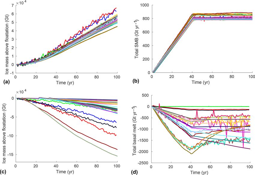
1444                                                           H. Seroussi et al.: An ice sheet model initialization experiment

   For the asmb and abmb experiments, anomalies in SMB              ables are values describing the entire ice sheet (e.g., ice mass,
and sub-shelf melt rates are applied in addition to the forcings    ice mass above floatation, and area-integrated SMB and basal
used in the init and ctrl experiments. The anomalies are ap-        melting). Three kinds of 2-D outputs are requested. State
plied as time-dependent functions, increasing stepwise each         variables (e.g., ice velocity and thickness) are snapshots re-
year over the first 40 simulation years and remaining constant      ported at a given time; flux variables are reported as temporal
over the last 60 years:                                             averages over a given period; and constant variables do not
                                                                    change with time.
                              [t]                                      Scalar outputs are provided for each simulation year and
EX(t) = EXctrl + EXanom ×         ; for 0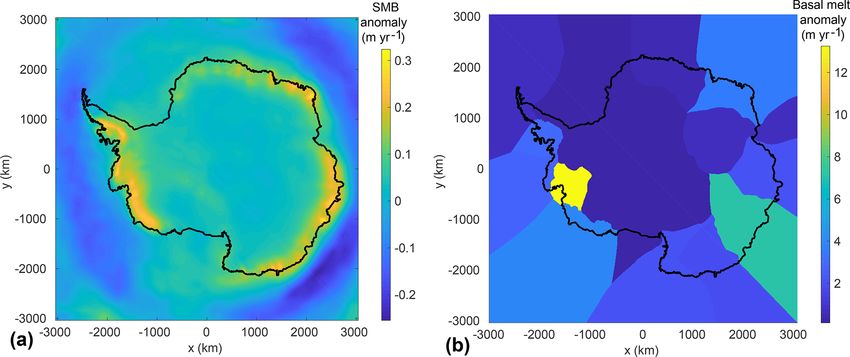
H. Seroussi et al.: An ice sheet model initialization experiment                                                             1445

Figure 1. (a) Surface mass balance anomaly (m yr−1 ) for the asmb experiment and (b) basal melt rate anomaly (m yr−1 ) for the abmb
experiment. Black contours show the current Antarctic ice extent.

described in Pollard and DeConto (2012a). Four models are           have retreat only where the ice melts completely (three sim-
based on a steady-state equilibrium in which the model is run       ulations).
for an extended period of time, until the ice sheet becomes
close to a steady-state equilibrium, with two models also in-
cluding present-day geometry as a target (Pollard and De-           4     Results
Conto, 2012a). The remaining seven initializations are based
                                                                    4.1    init experiment
on data assimilation, with three models also including a short
relaxation period after the data assimilation to limit the im-      Each model reports initial ice sheet conditions at the end of
pact of inconsistent datasets (Seroussi et al., 2011; Gillet-       the initialization procedure (init). The total ice-covered area
Chaulet et al., 2012).                                              varies between 1.35 × 10⁷ and 1.50 × 10⁷ km2 , a range of
   For the external SMB forcing, models use output from             only 10.5 % among models. The ice shelf extent, on the other
RACMO2 (Lenaerts et al., 2012), RACMO2.3 (van Wessem                hand, varies significantly among models, from 0.92 × 10⁶ to
et al., 2014), RACMO2.3p2 (van Wessem et al., 2018), MAR            2.51 × 10⁶ km2 , a range of 6.4 % to 16.7 % of the total ice-
(Agosta et al., 2019), ERA Interim (Dee et al., 2011), or           covered area. Figure 2 summarizes the initial extent of all
Arthern et al. (2006). Five simulations use a positive degree-      models. Some models have ice shelves hundreds of kilome-
day scheme (PDD; Reeh, 1991). These choices generate rel-           ters upstream or downstream of their current observed loca-
atively similar initial SMB (see Sect. 4). For sub-shelf melt-      tion. Although models generally agree on the location of the
ing, three simulations do not apply any melt rate. Four oth-        three largest ice shelves (Ross, Ronne–Filchner, and Amery),
ers apply values estimated from remote sensing, extrapolated        the location and extent of smaller shelves vary widely, in-
to regions that unground during the simulation. Most mod-           cluding in the Amundsen and Bellingshausen Sea sectors.
els apply a parameterization that depends linearly (Martin et       The initial ice mass above floatation varies from 1.79 × 10⁷
al., 2011; eight simulations) or quadratically (DeConto and         to 2.47×10⁷ Gt (between 49.4 and 68.1 m of SLE), while the
Pollard, 2016; four simulations) on the ocean thermal forc-         total ice mass varies from 2.11×10⁷ to 2.56×10⁷ Gt, in part
ing. Three simulations adjust the melt rate using an observed       because of the large discrepancy in ice shelf extent. Table C1
thickness target, and the remaining three simulations use the       details the main scalar variables in init for all simulations.
new Potsdam Ice-shelf Cavity model (PICO) parameteriza-                The ability of models to reproduce the characteristics of
tion (Reese et al., 2018).                                          the present-day ice sheet depends on their initialization pro-
   Most models include a moving ice front, but five simula-         cedure. The root mean square error (RMSE) between ob-
tions have a fixed ice front. Ice front migration is primarily      served (Fretwell et al., 2013) and modeled ice thickness
based on strain rate in most cases (Levermann et al., 2012;         varies between 91.2 and 422.3 m, with generally smaller er-
10 simulations). Some models use ice flux divergence and            rors (between 91.2 and 320.8 m) for models using data as-
accumulated damage at the ice front (Pollard et al., 2015;          similation or present-day geometry as a target in their ini-
three simulations), and some have ice-front retreat based on        tialization and larger errors (between 160.0 and 422.3 m) for
a threshold ice thickness (four simulations), while the others      models using spin-up, a steady state, or long relaxation pro-
                                                                    cedures without a geometry target (Fig. 3a). The RMSE be-

www.the-cryosphere.net/13/1441/2019/                                                     The Cryosphere, 13, 1441–1471, 2019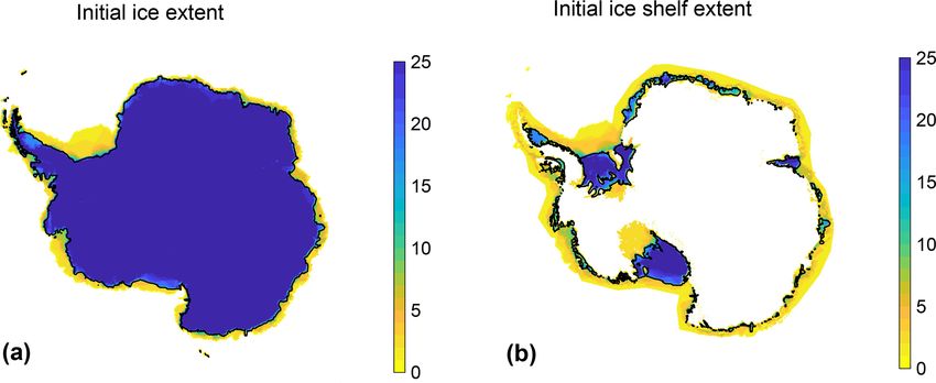
1446                                                             H. Seroussi et al.: An ice sheet model initialization experiment

Table 1. List of participants, modeling groups, and ice flow models in ISMIP6 initMIP-Antarctica.

         Contributors              Group ID     Ice flow model    Group
         Nicholas Golledge         ARC          PISM              Antarctic Research Centre,
         Daniel Lowry                                             Victoria University of Wellington, New Zealand
         Thomas Kleiner            AWI          PISM              Alfred Wegener Institute for Polar and Marine Research,
         Johannes Sutter                                          Bremerhaven, Germany
         Angelika Humbert
         Stephen Cornford          CPOM         BISICLES          Swansea University, UK
         Christian Rodehacke       DMI          PISM              Danish Meteorological Institute, Denmark
         Matthew Hoffman           DOE          MALI              Los Alamos National Laboratory, USA
         Tong Zhang
         Stephen Price
         Julien Brondex            IGE          Elmer/Ice         Institut des Géosciences de l’Environnement, France
         Fabien Gillet-Chaulet
         Ralf Greve                ILTS         SICOPOLIS         Institute of Low Temperature Science,
                                                                  Hokkaido University, Sapporo, Japan
         Heiko Goelzer             IMAU         IMAUICE           Institute for Marine and Atmospheric Research,
         Thomas Reerink                                           Utrecht, the Netherlands
         Roderik van de Wal
         Nicole Schlegel           JPL          ISSM              Jet Propulsion Laboratory, California Institute of Technology,
         Hélène Seroussi                                          Pasadena, USA
         Christophe Dumas          LSCE         Grisli            Laboratoire des Sciences du Climat et de l’Environnement,
         Aurélien Quiquet                                         Université Paris-Saclay, France
         Gunter Leguy              NCAR         CISM              National Center for Atmospheric Research, Boulder, CO, USA
         William Lipscomb
         Torsten Albrecht          PIK          PISM              Potsdam Institute for Climate Impact Research, Germany
         Matthias Mengel
         Ronja Reese
         Ricarda Winkelmann
         David Pollard             PSU          PSU               Earth and Environmental Systems Institute, Pennsylvania
                                                                  State University, University Park, PA, USA
         Mathieu Morlighem         UCIJPL       ISSM              University of California, Irvine, USA
         Helene Seroussi                                          Jet Propulsion Laboratory, California Institute of Technology,
                                                                  Pasadena, USA
         Frank Pattyn              ULB          f.ETISh           Université libre de Bruxelles, Belgium
         Sainan Sun
         Jonas Van Breedam         VUB          AISMPALEO         Vrije Universiteit Brussel, Belgium
         Philippe Huybrechts

tween observed (Rignot et al., 2011a) and modeled surface              are caused by large discrepancies in ice shelves and a few
velocity (Fig. 3b) also has a large spread among models,               fast-flowing ice streams: the RMSE for the logarithm of the
varying from 47.5 to 308 m yr−1 . These values are signifi-            speed, which emphasizes the slower-moving regions, varies
cantly affected by the inclusion of observed surface veloc-            only between 0.62 and 1.51 (Fig. 3c), or 3 times less than
ities during the initialization procedure: the RMSE in sur-            the RMSE of the speed. These errors are in part affected by
face speed varies from 47.5 to 94.5 m yr−1 for models in-              the exact year of the initialization procedure, as observations
cluding data assimilation of surface velocities and from 116           of velocity and thickness are not acquired at the same time.
to 308 m yr−1 for the other models. Most of these errors               However, the temporal variability of observed thickness and

The Cryosphere, 13, 1441–1471, 2019                                                         www.the-cryosphere.net/13/1441/2019/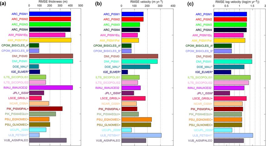
H. Seroussi et al.: An ice sheet model initialization experiment                                                                                1447

Table 2. List of initMIP-Antarctica simulations and main model characteristics. Numerics rely on the finite-difference (FD), finite-element
(FE), or finite-volume (FV) method. Initialization methods are as follows: spin-up (SP), spin-up with target values for the ice thickness (SP+;
see Pollard and DeConto, 2012a), data assimilation (DA), data assimilation with short relaxation (DA+), data assimilation of ice geometry
(DA∗ ), equilibrium state (Eq), and equilibrium state with target values for the ice thickness (Eq+). Initial SMB is derived from the following:
RACMO2 (RA2; Lenaerts et al., 2012), RACMO2.3 (RA2.3; van Wessem et al., 2014), RACMO2.3p2 (RA2.3p2; van Wessem et al., 2018),
MAR (Agosta et al., 2019), ERA Interim (ERA; Dee et al., 2011), Arthern et al. (2006) (Art), and positive degree-day schemes (PDD;
Reeh, 1991). Basal melt rates are based on zero melting (0), linear function of thermal forcing (Lin; Martin et al., 2011), quadratic function
of thermal forcing (Quad; DeConto and Pollard, 2016), melt rates estimated from observations (Obs; Rignot et al., 2013; Depoorter et al.,
2013), ice shelf thickness target (SS), ice shelf thickness target with no refreezing (SS∗ ), and the PICO parameterization (Reese et al., 2018).
Models that have partially floating cells at the grounding line apply melting using a sub-grid scheme (Sub-grid), a floatation condition to
assess if melt should be applied over the entire cell or not (Floating condition), or no melt at all (No) in their partially floating cells. Ice front
migration schemes are primarily based on strain rate (StR; Levermann et al., 2012), retreat only (RO), fixed front (Fix), minimum thickness
height (MH), and divergence and accumulated damage (Div; Pollard et al., 2015). The DMI_PISM1 and DMI_PISM0 differ by the basal
melt applied under the floating ice, with a basal melt reduced by an order of magnitude in DMI_PISM1 compared to DMI_PISM0. Further
details on all the models are given in Appendix B.

        n/a: not applicable.

velocity is small compared to the discrepancies between ob-                  poorter et al., 2013). Similar to the SMB forcing, these differ-
servations and models, so the exact year used for the initial                ences result from the chosen melting parameterization (Ta-
state has a limited impact on the RMSE calculated.                           ble 2) and the geometry of ice shelves.
   Area-integrated external forcings (SMB and basal melt)
also differ substantially among the models (see Table C1 in                  4.2    ctrl experiment
the Appendix C). The total initial SMB varies from 2015
to 3430 Gt yr−1 , depending on the origin of the SMB forc-                   Representing the current state of the ice sheet does not guar-
ing (see Table 2) and the extent of the ice-covered areas.                   antee that the current trends in ice sheet changes are correctly
The total initial ocean-induced basal melt varies from 0 to                  captured, which is what eventually matters in sea level rise
2470 Gt yr−1 , with seven models having values of less than                  projections. In the ctrl experiment, the Antarctic ice sheet
150 Gt yr−1 , while remote sensing estimates of total Antarc-                evolves under a constant climate for 100 years. The total
tic basal melt are ∼ 1400 Gt yr−1 (Rignot et al., 2013; De-                  change of ice mass above floatation varies from a loss of
                                                                             60 500 Gt to a gain of 88 100 Gt (i.e., 243 mm of SLE drop

www.the-cryosphere.net/13/1441/2019/                                                                  The Cryosphere, 13, 1441–1471, 2019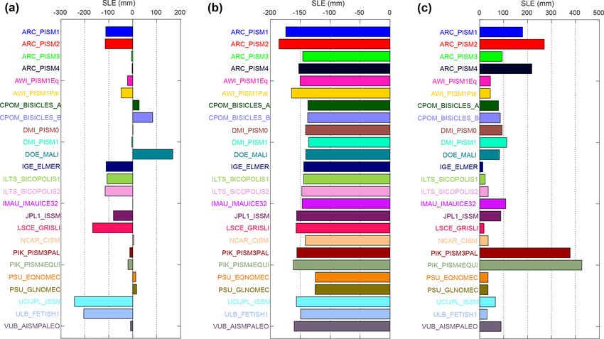
1448                                                                H. Seroussi et al.: An ice sheet model initialization experiment

Figure 2. Initial extent of ice-covered areas and ice shelves for all participating models. All contributions are regridded onto an 8 km standard
grid. Figures indicate how many models include ice (a, b) or floating ice (b) in each grid cell. Black lines show the observed ice extent (a) and
ice shelf extent (b) from Bedmap2 (Fretwell et al., 2013).

Figure 3. Root mean square error (RMSE) of modeled initial conditions compared to observations for (a) initial ice thickness (m), (b) initial
ice surface velocity (m yr−1 ) over the ice sheet and ice shelf, and (c) the logarithm of the initial ice surface velocity (log(m yr−1 )). Please
note that the model–color relationship used in this figure is applied in all subsequent figures. Models that assimilate present-day conditions
during their initialization process are denoted with + if they integrate geometry and ∗ if they integrate velocity and geometry information.

to 167 mm of SLE rise; see Fig. 4a and Table B2), with mass                an absolute change above 80 mm, and four have an abso-
loss in 8 simulations and gain in 17 simulations. This ab-                 lute change between 20 and 80 mm. All the models initial-
solute change in mass above floatation represents less than                ized with a steady-state equilibrium but one have a sea level
0.42 % of the initial volume in all cases, highlighting the                change lower than 20 mm, while all the models using data as-
accuracy required to calculate the Antarctic evolution for                 similation to determine their initial conditions but one have a
sea level projections. A spread of results is observed for all             sea level change above 80 mm. The models based on a paleo-
initialization methods and model resolutions. Eleven mod-                  climate spin-up have a large spread of sea level change in the
els have an absolute change lower than 20 mm, 10 have                      ctrl experiment and are present in all categories. The number

The Cryosphere, 13, 1441–1471, 2019                                                              www.the-cryosphere.net/13/1441/2019/
H. Seroussi et al.: An ice sheet model initialization experiment 1449
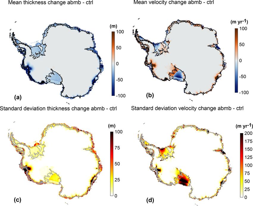
of models in each category is, however, relatively small to SMB anomaly spatial pattern (Fig. 1a), there is a thickening
draw definitive conclusions. of 3.6 m on average over Antarctica, with the largest changes
Figure 5 shows the spatial patterns of thickness and depth- happening along the West Antarctic coasts and the Antarc-
average horizontal ice speed for the ctrl experiment. Regrid- tic Peninsula (Fig. 8a). The standard deviation map (Fig. 8c)
ded results on the 8 km standard grid are used to compute shows that model differences are again concentrated along
modeled mean changes and standard deviation for these two the West Antarctica coast and on the Antarctic Peninsula.
variables. Results are reported only where at least five sim- The average standard deviation over the continent is 5.2 m
ulations have ice at a given grid point. Maps of thickness for this anomaly. The SMB anomaly has a small impact on
and velocity change during the ctrl experiment show that the ice dynamics, as shown in Fig. 8b, with a spatial average
signals are larger along the coast than in the interior of the speed increase of 1.5 m yr−1 over 100 years and a standard
continent and larger in West Antarctica compared to East deviation of 17.6 m yr−1 . Regions where models disagree are
Antarctica. The ice sheet mean thickness change, averaged similar to those for the ctrl experiment. Figure 9a compares
over all models, is equal to 1.2 m in 100 years. The standard for each model the difference in mass between the end of
deviation is calculated for each grid cell of the 8 km standard the asmb experiment and the end of the ctrl experiment with
grid based on the number of models reporting results in each the cumulative SMB anomaly of the asmb experiment inte-
cell and excluding cells where fewer than five models simu- grated over the entire ice sheet. It confirms that the additional
late ice. The standard deviation is much larger than the mean SMB is the primary cause of mass change: the SMB anomaly
changes in many places, with an average value over the simu- explains between 97 % and 130 % of the total mass change.
lated area of 14.8 m. Substantial thickening and thinning (es- The difference between the cumulative SMB anomaly and
pecially of ice shelves) compensate for each other, leading the change in mass is caused by thicker and faster ice (see
to a small spatial average change but large standard devia- Fig. 8) that increases the calving flux, as well as feedbacks
tion. Similarly, the spatial average velocity change is small, on ice shelf basal melt.
with a value of −1.9 m yr−1 , but the standard deviation is
27.4 m yr−1 . Some models have large accelerations in key re- 4.4 abmb experiment
gions, while others have large slowdowns. Regions with the
largest spread in model thickness and velocity changes are In the abmb experiment, an anomaly is applied to the basal
generally similar. melting rate of floating ice shelves, in addition to the basal
The ice extent is relatively temporally stable in all ctrl sim- melting used in the ctrl experiment. The basal melt anomaly
ulations, with less than 1.3 % change in the most sensitive is uniform within each region (see Fig. 1b) and largest in
simulations. Some simulations, however, have large tempo- the Amundsen Sea, where an additional ocean-induced melt
ral changes in ice shelf extent, ranging from a reduction of of 13.2 m yr−1 is applied. This additional melting leads to a
13 % to an increase of 14 %. The area-integrated SMB varies thinning of ice shelves, a reduction of the buttressing they
by up to 6 % for the simulations that experience the largest provide to grounded ice, an acceleration of the ice streams
change in SMB (Fig. 6b). The area-integrated basal melting feeding the shelves, and a retreat of grounding lines. How-
varies by more than 5 % for 15 models, with a maximum ever, unlike what is observed for the asmb experiment, the
change of 29 %, in response to changes in ice shelf extent abmb response varies significantly among models.
and thickness (Fig. 6c). Differences can be attributed in part to different treatments
of basal melt in model cells near the grounding line. Some
4.3 asmb experiment models have no melting in partially floating cells, others ap-
ply melt in partially floating cells based on the fraction of
In the asmb experiment, an SMB anomaly (Fig. 1a) is added floating area, and two models apply melt over the entire cell
to the SMB used in the ctrl experiment. This anomaly leads if it satisfies a floatation criterion (see Table 2). The spread in
to an increase in ice mass above floatation compared to ctrl, ice mass loss above floatation compared to the end of the ctrl
with the mass gain ranging from 4.51 × 10⁴ to 6.72 × 10⁴ Gt experiment varies by 2 orders of magnitude, from 4.7 × 10³
(125–186 mm decrease in SLE; see Fig. 4b). The differences to 1.5 × 10⁵ Gt (or 13–427 mm of SLE; see Fig. 4c and Ta-
among models (Fig. 7a, b) are linked to the extent of the ice- ble B2 in Appendix B), even though the additional melt is
covered areas, as well as ice shelf extent. For most models applied only to floating ice and therefore does not contribute
there is a small increase in grounded area, as some floating directly to sea level rise. The grounded area is reduced for all
areas near grounding lines thicken and reground due to the the models (between 0.10 % and 1.7 % reduction) as ground-
positive SMB anomaly. ing lines retreat. The change in ice shelf extent varies from a
Figure 8 shows the mean and standard deviation of the im- reduction of 25 % to an increase of 12 %, as some ice shelves
pact of this SMB anomaly on the ice thickness and depth- calve during this experiment, depending on the choice made
averaged horizontal velocity. Figure 8 is similar to Fig. 5 but for ice front evolution (see Table 2).
for the difference between the end of the asmb experiment Figure 10 shows that the modeled mean and standard de-
and the end of the ctrl experiment. As expected from the viation for the ice thickness and depth-averaged velocity
www.the-cryosphere.net/13/1441/2019/ The Cryosphere, 13, 1441–1471, 2019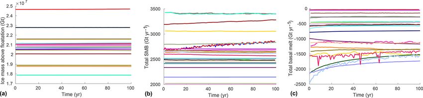
1450 H. Seroussi et al.: An ice sheet model initialization experiment
Figure 4. Antarctic contribution to sea level (mm of sea level equivalent). (a) ctrl experiment, (b) difference between asmb and ctrl experi-
ments, and (c) difference between abmb and ctrl experiments. Negative values of SLE represent a growing ice sheet.
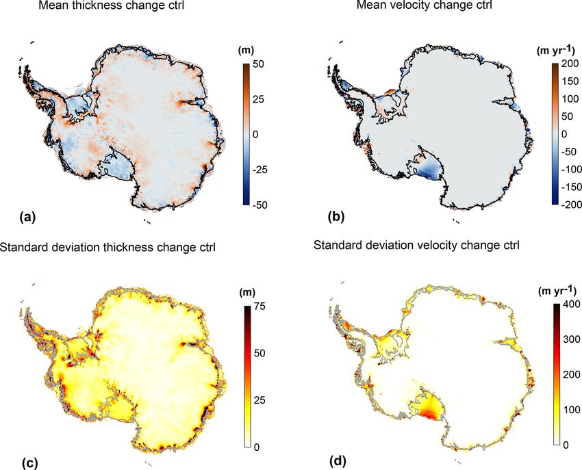
changes are concentrated on the ice shelves and near ground- 5 Discussion
ing lines. Ice thinning is 10.7 m on average, and the standard
deviation is 12.4 m. The dynamic impact of such variations is
not limited to the ice shelves but propagates upstream of the
grounding line, especially in the Amundsen Sea Basin, where The initMIP-Antarctica experiments are designed to analyze
the largest anomalies are applied. The Ross and Filchner– the impact of ice sheet model initial conditions on the evolu-
Ronne ice shelves have acceleration near the grounding line tion of the Antarctic ice sheet and its response to simple cli-
but also a slowdown near the ice front. The modeled mean mate forcings. For this exercise, 16 groups submitted 25 sim-
velocity change over the ice sheet is a small slowdown of ulations, more than 4 times the number of Antarctic simu-
3.3 m yr−1 ; this signal is small compared to the standard de- lations submitted for the SeaRISE project (Bindschadler et
viation of 29.6 m yr−1 . Regions where models show a large al., 2013), highlighting the importance and the fast evolution
spread of thickness and velocity changes are different from of this research field (Pattyn et al., 2017). The simulations
the ctrl and asmb simulations. Large deviations among mod- represent a large diversity of initialization methods, forcing
els extend upstream from the present-day grounding lines datasets, and model parameters, and the results show a large
and over the ice streams feeding the ice shelves, reflecting spread in the mass balance and dynamic evolution of this ice
different model responses to this oceanic forcing. Figure 9b sheet in century-scale simulations.
compares for each model the difference in mass between the The initial ice volume above floatation varies from 1.8 to
end of the abmb experiment and the end of the ctrl experi- 2.5 × 10⁷ Gt, or almost 32 %, which is much larger than the
ment, with the cumulative basal melt anomaly of the abmb spread of about 8 % in SeaRISE (Nowicki et al., 2013b). This
experiment integrated over the entire ice sheet. It shows that is not surprising given the larger number of model contri-
the additional basal melt only accounts for a fraction of the butions. On the other hand, the largest drifts in the ctrl ex-
mass change: the basal melt anomaly explains between 5 % periment are reduced compared to the SeaRISE project. For
and 125 % of the total mass change. The difference between initMIP-Antarctica, the ctrl sea level contribution varies be-
the cumulative basal melt anomaly and the change in mass is tween −243 and +167 mm of sea level equivalent for the
mainly caused by thinner and slower ice shelves (see Fig. 10) 25 simulations of ISMIP6, while its evolution varied between
that reduce the calving flux. −256 and +1 mm over the first 100 years for the six simu-
lations of SeaRISE. Specifically, four models participated in
both SeaRISE and initMIP-Antarctica, and the large drift that
The Cryosphere, 13, 1441–1471, 2019 www.the-cryosphere.net/13/1441/2019/H. Seroussi et al.: An ice sheet model initialization experiment 1451 Figure 5. Mean (a, b) and standard deviation (c, d) of the change in ice thickness (a and c, in m) and depth-averaged horizontal velocity (b and d, in m yr−1 ) between the beginning and end of the ctrl experiment. Black (a, c) or grey (b, d) lines show the observed current ice front and grounding line positions. Figure 6. Evolution of Antarctic ice sheet mass above floatation and external forcings in the ctrl experiment. (a) Total mass of ice above floatation (Gt), (b) total SMB applied at the ice surface (Gt yr−1 ), and (c) total basal melting rate (Gt yr−1 ). two of them experienced in SeaRISE has been reduced in the SMB anomaly in initMIP-Greenland. In Greenland, large ab- initMIP-Antarctica ctrl experiment. lation rates are applied at the ice sheet periphery, leading to The asmb and abmb experiments are designed to analyze significant ice loss for the models with the largest initial ex- the ice sheet response to simple anomalies in SMB and basal tents (Goelzer et al., 2018). The Antarctic SMB anomaly has melting under the ice shelves. Unlike initMIP-Greenland, less spatial variability, and the initial extent of the ice sheet where Goelzer et al. (2018) observed a large spread of 118 % is closer for the different simulations, which leads to more in the responses in the asmb experiment, the response to the consistent responses to this perturbation. SMB anomaly in initMIP-Antarctica is similar among all the While the response to the SMB anomaly has limited varia- models, with a 39 % variation in the response to this anomaly tions among models, the impact of the basal melting anomaly between the models. The differences can be attributed to the varies significantly among models, with a spread in sea level larger spread in initial ice sheet extent and the pattern of the contribution from 13 mm to more than 400 mm. Several fac- www.the-cryosphere.net/13/1441/2019/ The Cryosphere, 13, 1441–1471, 2019
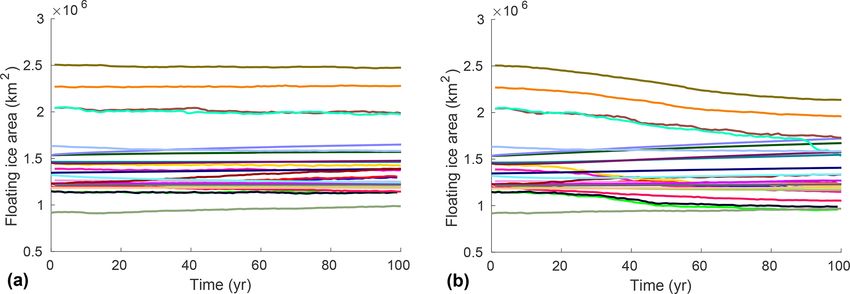
1452                                                             H. Seroussi et al.: An ice sheet model initialization experiment

Figure 7. Evolution of the Antarctic ice sheet and external forcings in the asmb (a and b) and abmb (c and d) experiments compared to the
ctrl experiment. Total amount of ice above floatation for asmb minus ctrl (a) and abmb minus ctrl (c) (in Gt). Evolution of SMB applied at
the ice surface for asmb minus ctrl (b, in Gt yr−1 ) and total basal melting applied in abmb minus ctrl (d, in Gt yr−1 ).

tors explain the wide range of abmb responses. First, mod-             ble B1). As the basal melting anomaly is applied only un-
els vary in their treatment of basal melting near the ground-          der floating ice, the spatial extent and amount of the applied
ing line. Elements and grid cells crossed by the grounding             anomaly therefore vary significantly from one model to the
line are considered partially floating. Some models have no            next. Ice shelf extent also varies during the ctrl and abmb
melting in partially floating cells, others apply melt in par-         experiments, so that the applied melt anomaly evolves differ-
tially floating cells based on the fraction of floating area, and      ently between the simulations. As shown in Fig. 11, floating
two models apply melt over the entire cell if it satisfies a           ice areas stay relatively constant in some models, increase
floatation criterion (see Table 2). These different treatments         because of grounding line retreat in others, and decrease as
can have a significant impact on grounding line evolution, as          ice shelves thin significantly and calve in the remaining ones.
highlighted by previous studies (Arthern and Williams, 2017;              Third, while the SMB applied in init and ctrl is relatively
Seroussi and Morlighem, 2018). This is especially important            similar among the different models, the basal melting varies
for continental-scale simulations that have a resolution vary-         from zero melt to 2140 Gt yr−1 . The latter value is about
ing between several kilometers and several tens of kilome-             50 % larger than values derived from remote sensing ob-
ters, as is the case in initMIP-Antarctica. The four largest           servations (Rignot et al., 2013; Depoorter et al., 2013) (see
sea level contributions in the abmb experiment (> 200 mm)              Fig. 7). The applied basal melting anomaly therefore repre-
come from four models that apply sub-grid melt in par-                 sents about half the initial basal melting for some models but
tially floating cells and have a resolution of 8 km or coarser         a drastic increase for others. The impact on ice shelf thick-
(see Tables 2 and B2). Additionally, two of these models               ness evolution and dynamic response is therefore very differ-
were run without (ARC_PISM1 and ARC_PISM3) and with                    ent, as shown by Fig. 10.
(ARC_PISM2 and ARC_PISM4) a sub-grid melt scheme in                       Finally, surface-elevation feedback processes were not al-
partially floating cells (see Table 2), which resulted in an ad-       lowed in asmb, ensuring that a similar SMB anomaly was ap-
ditional sea level rise of 90 and 124 mm when the sub-grid             plied by all models at a given location. In abmb, no such con-
melt scheme was used.                                                  straint was prescribed, which introduces feedbacks between
   Second, the total ice shelf extent varies by more than              ice shelf and basal melting for some parameterizations. For
100 % among the different models, and their extent within              example, if an ice shelf thins and the grounding line retreats
different basins also varies significantly (see Fig. 2 and Ta-         in a given model, the newly floating ice experiences basal

The Cryosphere, 13, 1441–1471, 2019                                                          www.the-cryosphere.net/13/1441/2019/
H. Seroussi et al.: An ice sheet model initialization experiment                                                                      1453

Figure 8. Mean (a, b) and standard deviation (c, d) of the ice thickness (a and c, in m) and depth-averaged horizontal velocity (b and d,
in m yr−1 ) between the end of the asmb experiment and the end of the ctrl experiment. Black (a, b) or grey (c, d) lines show the current
observed ice front and grounding line positions.

Figure 9. (a) Difference in mass (Gt) between the end of the asmb experiment and the end of the ctrl experiment and the cumulative SMB
anomaly (Gt) of the asmb experiment integrated over the entire ice sheet for the 25 simulations. (b) Difference in mass (Gt) between the end
of the abmb experiment and the end of the ctrl experiment and the cumulative basal melt anomaly (Gt) of the abmb experiment integrated
over the entire ice sheet for the 25 simulations. Black dashed lines show mass change equal to cumulative anomaly change.

www.the-cryosphere.net/13/1441/2019/                                                           The Cryosphere, 13, 1441–1471, 2019
1454                                                              H. Seroussi et al.: An ice sheet model initialization experiment

Figure 10. Mean (a, b) and standard deviation (c, d) of the change in ice thickness (a and c, in m) and depth-averaged horizontal velocity
(b and d, in m yr−1 ) between the end of the abmb experiment and the end of the ctrl experiment. Black (a, b) or grey (c, d) lines show the
current observed ice front and grounding line positions.

melting that can drive further thinning and retreat. The effec-         ing to combine them by either following data assimilation
tive basal melting anomaly therefore varies between the sim-            with short relaxation periods or by assimilating surface ele-
ulations (see Fig. 7d). These results highlight the need for            vation during transient initialization to have an initial geome-
further modeling studies and observations on basal melting              try more consistent with observations (Pollard and DeConto,
patterns near the grounding line.                                       2012a). Combining the best of both approaches is an active
   One objective of ISMIP6 and initMIP-Antarctica is to                 field of research. Assimilating observations over longer time
gather a large and diverse ice sheet modeling community. To             periods looks like a promising option, despite the technical
facilitate participation of a large number of models, only two          challenges (Larour et al., 2014; Goldberg et al., 2015).
constraints were imposed: (1) the inclusion of both grounded               Representation of ice shelves and their connection to
and floating ice and (2) the simulation of dynamic ground-              glaciers upstream is an outstanding cause of differences
ing line migration. This lack of constraints complicates the            among models. Ice shelves are directly affected by varia-
analysis of the simulation differences, since model param-              tions in oceanic (Jacobs et al., 2011; Pritchard et al., 2012;
eters, input forcing, initialization techniques, and physical           Greenbaum et al., 2015; Wouters et al., 2015) and atmo-
processes vary widely among models. Initialization methods              spheric (Scambos et al., 2000; Banwell et al., 2013; Munneke
that are based on the assimilation of present-day conditions            et al., 2014; Bassis and Ma, 2015) conditions, which impacts
usually have lower RMSE in the initial ice thickness and ve-            grounding line and ice front evolution (Favier et al., 2014;
locity compared to observations (Fig. 3) but larger trends              Joughin et al., 2014; Rignot et al., 2014; Bassis and Ma,
in the ctrl experiment (Fig. 4a), while the opposite is true            2015; Scheuchl et al., 2016; Christie et al., 2016; Seroussi
for models relying on paleoclimate spin-up or a steady-state            et al., 2017). Ice shelf evolution over the past few decades
solution. This is similar to what was previously observed               has been complex, with large spatial and temporal variabil-
by Nowicki et al. (2013a, b) and Goelzer et al. (2018). As              ity (Depoorter et al., 2013; Rignot et al., 2013; Paolo et al.,
the two approaches are complementary, models are start-                 2015; Christie et al., 2018) that is not fully understood and

The Cryosphere, 13, 1441–1471, 2019                                                          www.the-cryosphere.net/13/1441/2019/
H. Seroussi et al.: An ice sheet model initialization experiment                                                                      1455

Figure 11. Evolution of Antarctic ice shelf extent for the (a) ctrl and (b) abmb experiments.

typically is not included in numerical models. Representation            broad participation, with 25 model simulations submitted
of ice shelves varies among models: the ice shelf extent, spa-           from 16 groups. Results are improved compared to previ-
tial location, and thickness differ significantly between the            ous similar exercises of continental-scale modeling of the
simulations, resulting in large deviations in ice shelf flow.            Antarctic ice sheet, with enhanced representation of present-
Another major source of disagreement is the boundary con-                day conditions and ice mass loss trend. A first experiment
dition at the ice–ocean interface, with ocean-induced basal              performed with a simple surface mass balance anomaly forc-
melting applied under the floating ice and its temporal evo-             ing produces relatively robust results across the models,
lution based on a wide range of parameterizations. Signifi-              while a second experiment with a simple perturbation in
cant progress was made over the past decade (Pattyn et al.,              basal melting rate under the ice shelves creates very large
2017), but continued improvement of ice shelf representation             discrepancies in the ice sheet response. Variations in the rep-
in continental-scale models should remain a research priority            resentation of ice shelves (e.g., spatial extent, thickness), ice
so that ice shelf representation in continental-scale ice sheet          shelf basal melting, and numerical treatment of grounding
models is in better agreement with observations of the cur-              lines cause this significant spread of results between the sim-
rent state of the Antarctic ice sheet.                                   ulations. Including accurate representations of ice shelves
   The results presented in this study rely on simple atmo-              that are consistent with observations of the current Antarc-
spheric and oceanic forcings that are only loosely based on              tic ice sheet in continental-scale models should therefore re-
RCP scenarios. Furthermore, many participating models did                main an important research subject in the coming years. All
not use their full capabilities. To reduce model differences,            the experiments performed as part of initMIP-Antarctica are
for example, participants were asked to turn off surface-                based on simplified anomaly forcings. Future projections of
elevation feedback schemes, bedrock adjustment capabili-                 the Antarctic ice sheet evolution under different climate sce-
ties, and ice cliff failure. As a result, the initMIP-Antarctica         narios are currently being designed and will be the subject of
simulations are not projections of Antarctic evolution over              future ISMIP6 modeling experiments.
the coming century and should not be compared with pre-
vious Antarctic simulations aiming to simulate this evolution
(e.g., Ritz et al., 2015; Golledge et al., 2015). The next step of       Data availability. The model output from the simulations de-
ISMIP6 will be the assessment of Antarctic evolution under               scribed in this paper and forcing data sets will be made publicly
different scenarios forced with oceanic and atmospheric con-             available with a digital object identifier https://doi.org/10.5281/
ditions derived from CMIP climate models; experiments are                zenodo.2651652. In order to document CMIP6’s scientific impact
                                                                         and enable ongoing support of CMIP, users are asked to acknowl-
now being designed. The initMIP-Antarctic simulations do,
                                                                         edge CMIP6, ISMIP6, and the participating modeling groups.
however, illustrate the spread in ice sheet evolution (hence
sea level) that is due to ice sheet model initial state and mod-
eling choices (e.g., grounding line numerics, calving laws)
and provide insight into uncertainty in simulations of sea
level change.

6   Conclusions

The initMIP-Antarctica experiment, part of the Ice Sheet
Model Intercomparison Project for CMIP6 (ISMIP6), had

www.the-cryosphere.net/13/1441/2019/                                                            The Cryosphere, 13, 1441–1471, 2019
1456 H. Seroussi et al.: An ice sheet model initialization experiment
Appendix A: Outputs and output format
initMIP-Antarctica participants are required to provide out-
put variables according to the data request plan. Three types
of 2-D fields are reported by modeling groups at 5-year in-
tervals: state variables, flux variables, and constants. Also,
scalar outputs (e.g., total ice mass, ice mass above floatation,
SMB, basal melt) are reported every simulation year. Table
A1 provides the complete list of requested variables. In ad-
dition to model output results, a README file describing
model characteristics and details of the initialization proce-
dure was requested from modeling groups for each simula-
tion.
Table A1. Data requests for initMIP-Antarctica. ST: state variable. FX: flux variable. CST: constant.
Variable name Type Standard name Unit
Ice sheet thickness ST land_ice_thickness m
Ice sheet surface elevation ST surface_altitude m
Ice sheet base elevation ST base_altitude m
Bedrock elevation ST bedrock_altitude m
Geothermal heat flux CST upward_geothermal_heat_flux_at_ground_level W m−2
Surface mass balance flux FL land_ice_surface_specific_mass_balance_flux kg m−2 s−1
Basal mass balance flux FL land_ice_basal_specific_mass_balance_flux kg m−2 s−1
Ice thickness imbalance FL tendency_of_land_ice_thickness m s−1
Surface velocity in x direction ST land_ice_surface_x_velocity m s−1
Surface velocity in y direction ST land_ice_surface_y_velocity m s−1
Surface velocity in z direction ST land_ice_surface_upward_velocity m s−1
Basal velocity in x direction ST land_ice_basal_x_velocity m s−1
Basal velocity in y direction ST land_ice_basal_y_velocity m s−1
Basal velocity in z direction ST land_ice_basal_upward_velocity m s−1
Mean velocity in x direction ST land_ice_vertical_mean_x_velocity m s−1
Mean velocity in y direction ST land_ice_vertical_mean_y_velocity m s−1
Ice surface temperature ST temperature_at_ground_level_in_snow_or_firn K
Ice basal temperature ST land_ice_basal_temperature K
Magnitude of basal drag ST magnitude_of_land_ice_basal_drag Pa
Land ice calving flux FL land_ice_specific_mass_flux_due_to_calving kg m−2 s−1
Grounding line flux FL land_ice_specific_mass_flux_due_at_grounding_line kg m−2 s−1
Land ice area fraction ST land_ice_area_fraction 1
Grounded ice sheet area fraction ST grounded_ice_sheet_area_fraction 1
Floating ice sheet area fraction ST floating_ice_sheet_area_fraction 1
Total ice sheet mass ST land_ice_mass kg
Total ice sheet mass above floatation ST land_ice_mass_not_displacing_sea_water kg
Area covered by grounded ice ST grounded_land_ice_area m2
Area covered by floating ice ST floating_ice_shelf_area m2
Total SMB flux FL tendency_of_land_ice_mass_due_to_surface_mass_balance kg s−1
Total BMB flux FL tendency_of_land_ice_mass_due_to_basal_mass_balance kg s−1
Total calving flux FL tendency_of_land_ice_mass_due_to_calving kg s−1
Total grounding line flux FL tendency_of_grounded_ice_mass kg s−1
The Cryosphere, 13, 1441–1471, 2019 www.the-cryosphere.net/13/1441/2019/H. Seroussi et al.: An ice sheet model initialization experiment 1457
Appendix B: Model description and initialization forcing (PISM1Pal), time slice anomalies for the Last Inter-
glacial (LIG) and the Last Glacial Maximum (LGM) from
Below are descriptions of the ice flow models and the initial- the Earth System Model COSMOS (Pfeiffer and Lohmann,
ization procedure performed by the different groups. 2016; Zhang et al., 2014) are used in addition to datasets
for present-day (PD) Antarctic climate (RACMO2.3, van
B1 ARC_PISM Wessem et al., 2014; WOA09, Locarnini et al., 2010). Time-
dependent and spatially variable climate anomaly fields are
We use the Parallel Ice Sheet Model (PISM) version 0.7.1. interpolated during the PISM run between LIG, LGM, and
PISM is a hybrid ice sheet–ice shelf model that combines PD climate time slices with a glacial index method (Sut-
shallow approximations of the flow equations that compute ter et al., 2016), where the glacial index is derived from
gravitational flow and flow by horizontal stretching (Bueler Dome C deuterium depletion (Jouzel et al., 2007). For the
and Brown, 2009). We perform two sets of experiments with SMB, PISM’s positive degree-day (PDD) scheme is used.
different initialization procedures. In the first set (PISM-1,2), Relative sea level forcing (Waelbroeck et al., 2002) and bed
the simulations are initialized from the end of a 120 000-year deformation (Bueler et al., 2007) are applied during the pa-
spin-up using paleoclimate forcing, whereas in the second leo spin-up. In addition to the paleo spin-up, a 100 ka-long
set (PISM-3,4), the simulations are initialized from the end equilibrium-type spin-up (PISM1Eq) with steady present-
of a 100 000-year spin-up using a constant climate forcing. day climate (ocean and atmosphere) and sea level is car-
Both procedures result in a present-day ice sheet configura- ried out with isostatic bed deformation. Instead of precipi-
tion that is in a thermally and dynamically evolved state, with tation and 2 m air temperature (PISM1Pal), SMB and skin
a “present-day” sea-level equivalent volume of 58.35 and temperature from RACMO2.3 are directly applied without
56.38 m, respectively. The combined stress balance of PISM the PDD scheme. The initial geometry for both spin-ups is
allows for a treatment of ice sheet flow that is consistent Bedmap2 (Fretwell et al., 2013), and the geothermal flux is
across non-sliding grounded ice to rapidly sliding grounded from Shapiro and Ritzwoller (2004). Basal shelf melt rates
ice (ice streams) and floating ice (shelves). As with most are calculated via a quadratic form of the melt rate formula
continental-scale ice sheet models, we use flow enhancement in Beckmann and Goosse (2003) using the extrapolated 3-D
factors for the shallow-ice and shallow-shelf components of ocean temperatures at the depth of the ice shelf base. PISM’s
the stress regime (3.5 and 0.5, respectively, for PISM-1,2, sub-grid grounding line scheme for basal sliding (Feldmann
and 2.8 and 0.5, respectively, for PISM-3,4), which allow et al., 2014) is used in all simulations.
us to adjust creep and sliding velocities using simple coeffi-
cients. By doing so we are able to optimize simulations such
B3 CPOM_BISICLES
that modeled behavior is consistent with observed behavior.
The junction between grounded and floating ice is refined
by a sub-grid-scale parameterization (Feldmann et al., 2014) CPOM_BISICLES_A_500m is a block structured adaptive
that smooths the basal shear stress field and tracks an inter- mesh finite-element model based on a vertically integrated
polated grounding-line position through time. This allows for stress balance model (Cornford et al., 2013, 2016) and the
much more realistic grounding-line motion, even with rela- basal friction physics of Tsai et al. (2015). Here, we make
tively coarse spatial grids, such as the 16 km grid used in use of the adaptive mesh to maintain a resolution of 8 km
our experiments. We run duplicate experiments with the sub- in the slow-moving interior, 1 km in ice streams, and 500 m
grid melt turned off (PISM-1,3) or on (PISM-2,4) in order at the grounding line. The initial state is based on ice thick-
to quantify the effect of this scheme. SMB is calculated us- ness and bedrock elevation from Bedmap2 (Fretwell et al.,
ing a positive degree-day model that takes as inputs air tem- 2013), modified according to mass conservation close to the
perature and precipitation from RACMO2.1 (Lenaerts et al., grounding line to avoid the large unphysical thickening rates
2012). In previous simulations (e.g., Golledge et al., 2015) that would otherwise occur, especially in the Amundsen Sea
we have derived evolving melt beneath ice shelves from the Embayment. Ice temperature is taken from Pattyn (2010) and
thermodynamic three-equation model of Hellmer and Ol- is held constant in time over the course of the simulations.
ber (1989), in which the melt rate is primarily controlled by Effective viscosity ϕ(x, y) and effective drag coefficients
salinity and temperature gradients across the ice–ocean inter- β 2 (x, y) are estimated by minimizing the mismatch between
face. For the simplified experiments presented here, however, modeled speed the observed speed of Rignot et al. (2011b),
we set a spatially uniform melt rate as an initial condition and following the methods described in Cornford et al. (2015)
allow our modeled ice sheet to evolve in response to this. The background ocean melt rate M0 (x, y, t) is defined so that
the thinning rate is zero across the ice shelf and varies in time
B2 AWI_PISM accordingly, so that when a melt rate anomaly Ma (x, y, t) is
applied, the ice shelf thinning rate is Ma (x, y, t).
The simulations are performed with PISM version 0.7.3. CPOM_BISICLES_B is similar to CPOM_BISICLES_A
For the 220 ka-long spin-up simulations with paleoclimatic but does not allow accumulation onto the lower surface of the
www.the-cryosphere.net/13/1441/2019/ The Cryosphere, 13, 1441–1471, 2019You can also read