Freshwater pearl mussels from northern Sweden serve as long-term, high-resolution stream water isotope recorders
←
→
Page content transcription
If your browser does not render page correctly, please read the page content below
Hydrol. Earth Syst. Sci., 24, 673–696, 2020
https://doi.org/10.5194/hess-24-673-2020
© Author(s) 2020. This work is distributed under
the Creative Commons Attribution 4.0 License.

Freshwater pearl mussels from northern Sweden serve as long-term,
high-resolution stream water isotope recorders
Bernd R. Schöne1 , Aliona E. Meret2 , Sven M. Baier3 , Jens Fiebig4 , Jan Esper5 , Jeffrey McDonnell6 , and
Laurent Pfister7
1 Institute of Geosciences, University of Mainz, Mainz, 55128, Germany
2 Naturhistoriska  riksmuseet, Stockholm, 114 18, Sweden
3 Agilent Technologies Sales & Services GmbH & Co. KG, Frankfurt am Main, 60528, Germany
4 Institute of Geosciences, J. W. Goethe University, Frankfurt am Main, 60438, Germany
5 Department of Geography, University of Mainz, Mainz, 55128, Germany
6 Global Institute for Water Security, University of Saskatchewan, Saskatoon, SK S7N 3H5, Canada
7 University of Luxembourg, Faculty of Science, Technology and Medicine, 2 Avenue de l’Université,

4365, Esch-sur-Alzette, Luxembourg

Correspondence: Bernd R. Schöne (schoeneb@uni-mainz.de)

Received: 29 June 2019 – Discussion started: 29 July 2019
Revised: 27 November 2019 – Accepted: 16 January 2020 – Published: 17 February 2020

Abstract. The stable isotope composition of lacustrine sed-       consistent ontogenetic trends, but rather oscillated around an
iments is routinely used to infer Late Holocene changes in        average that ranged from ca. −12.00 to −13.00 ‰ among
precipitation over Scandinavia and, ultimately, atmospheric       the streams studied. Results of this study contribute to an
circulation dynamics in the North Atlantic realm. However,        improved understanding of climate dynamics in Scandinavia
such archives only provide a low temporal resolution (ca.         and the North Atlantic sector and can help to constrain eco-
15 years), precluding the ability to identify changes on inter-   hydrological changes in riverine ecosystems. Moreover, long
annual and quasi-decadal timescales. Here, we present a           isotope records of precipitation and streamflow are pivotal
new, high-resolution reconstruction using shells of freshwa-      to improve our understanding and modeling of hydrological,
ter pearl mussels, Margaritifera margaritifera, from three        ecological, biogeochemical and atmospheric processes. Our
streams in northern Sweden. We present seasonally to annu-        new approach offers a much higher temporal resolution and
ally resolved, calendar-aligned stable oxygen and carbon iso-     superior dating control than data from existing archives.
tope data from 10 specimens, covering the time interval from
1819 to 1998. The bivalves studied formed their shells near
equilibrium with the oxygen isotope signature of ambient
water and, thus, reflect hydrological processes in the catch-     1   Introduction
ment as well as changes, albeit damped, in the isotope sig-
nature of local atmospheric precipitation. The shell oxygen       Multi-decadal records of δ 18 O signals in precipitation and
isotopes were significantly correlated with the North Atlantic    stream water are important for documenting climate change
Oscillation index (up to 56 % explained variability), suggest-    impacts on river systems (Rank et al., 2017), improving the
ing that the moisture that winter precipitation formed from       mechanistic understanding of water flow and quality control-
originated predominantly in the North Atlantic during NAO+        ling processes (Darling and Bowes, 2016), and testing Earth
years but in the Arctic during NAO− years. The isotope sig-       hydrological and land surface models (Reckerth et al., 2017;
nature of winter precipitation was attenuated in the stream       Risi et al., 2016; see also Tetzlaff et al., 2014). However, the
water, and this damping effect was eventually recorded by         common sedimentary archives used for such purposes typi-
the shells. Shell stable carbon isotope values did not show       cally do not provide the required, i.e., at least annual, tem-
                                                                  poral resolution (e.g., Rosqvist et al., 2007). In such stud-

Published by Copernicus Publications on behalf of the European Geosciences Union.
674          B. R. Schöne et al.: Freshwater pearl mussels as long-term, high-resolution stream water isotope recorders

ies, the temporal changes in the oxygen isotope signatures         80 years (von Hessling, 1859) to over 200 years (Ziuganov
of meteoric water are encoded in biogenic tissues and abio-        et al., 2000; Mutvei and Westermark, 2001), offering an in-
genic minerals formed in rivers and lakes (e.g., Teranes and       sight into long-term changes in freshwater ecosystems at an
McKenzie, 2001; Leng and Marshall, 2004). In fact, many            unprecedented temporal resolution.
studies have determined the oxygen isotope composition of             Here, we present the first absolutely dated, annually re-
diatoms, ostracods, authigenic carbonate and aquatic cellu-        solved stable oxygen and carbon isotope record of freshwater
lose preserved in lacustrine sediments to reconstruct Late         pearl mussels from three different streams in northern Swe-
Holocene changes in precipitation over Scandinavia and, ul-        den covering nearly 2 centuries (1819–1998). We test the
timately, atmospheric circulation dynamics in the North At-        ability of these freshwater pearl mussels to reconstruct the
lantic realm (e.g., Hammarlund et al., 2002; Andersson et al.,     NAO index and associated changes in precipitation prove-
2010; Rosqvist et al., 2004, 2013). With their short residence     nance using shell oxygen isotope data (δ 18 Os ). We evalu-
times of a few months (Rosqvist et al., 2013), the hydro-          ate how shell oxygen isotope data compare to δ 18 O values
logically connected, through-flow lakes of northern Scandi-        in stream water (δ 18 Ow ) and precipitation (δ 18 Op ) as well
navia are an ideal region for this type of study. Their isotope    as limited existing environmental data (such as stream wa-
signatures – while damped in comparison with isotope sig-          ter temperature); we also evaluate how these variables relate
nals in precipitation – directly respond to changes in the pre-    to each other. We hypothesize that δ 18 Ow and δ 18 Op values
cipitation isotope composition (Leng and Marshall, 2004).          are positively correlated with one another as well as with
However, even the highest available temporal resolution of         the North Atlantic Oscillation index. In other words, during
such records (15 years per sample in sediments from Lake           positive NAO years, oxygen isotope values in stream wa-
Tibetanus, Swedish Lapland; Rosqvist et al., 2007) is still        ter and shells are higher than during negative NAO years,
insufficient to resolve inter-annual- to decadal-scale variabil-   when shell and stream water oxygen isotope values tend to
ity, i.e., the timescales at which the North Atlantic Oscilla-     be more depleted in 18 O. In addition, we explore the phys-
tion (NAO) operates (Hurrell, 1995; Trouet et al., 2009). The      ical controls on shell stable carbon isotope signatures. Pre-
NAO steers weather and climate dynamics in northern Scan-          sumably, these data reflect changes in the stable carbon iso-
dinavia and determines the origin of air masses from which         tope value of dissolved inorganic carbon, which, in turn, is
meteoric waters form. While sediment records are still of vi-      sensitive to changes in primary production. We leverage past
tal importance for century-scale and millennial-scale varia-       work in Sweden that has shown that the main growing season
tions, new approaches are needed for finer-scale resolution        of M. margaritifera occurs from mid-May to mid-October,
on the 1–100-year timescale.                                       with the fastest growth rates occurring between June and Au-
    One underutilized approach for hydroclimate reconstruc-        gust (Dunca and Mutvei, 2001; Dunca et al., 2005; Schöne et
tion is the use of freshwater mussels as natural stream water      al., 2004a, b, 2005a). We use changes in the annual incre-
stable isotope recorders (Dettman et al., 1999; Kelemen et al.,    ment width of M. margaritifera to infer water temperature,
2017; Pfister et al., 2018, 2019). Their shells can provide sea-   because growth rates are faster during warm summers and
sonally to annually resolved, chronologically precisely con-       result in broader increment widths (Schöne et al., 2004a, b,
strained records of environmental changes in the form of           2005a). Because specimens of a given population react sim-
variable increment widths (which refers to the distance be-        ilarly to changes in temperature, their average shell growth
tween subsequent growth lines) and geochemical properties          patterns can be used to estimate climate and hydrological
(e.g., Nyström et al., 1996; Schöne et al., 2005a; Geist et al.,   changes. Consequently, increment series of specimens with
2005; Black et al., 2010; Schöne and Krause, 2016; Geeza           overlapping life spans can be crossdated and combined to
et al., 2019, 2020; Kelemen et al., 2019). In particular, sim-     form longer chronologies covering several centuries (Schöne
ilar to marine (Epstein et al., 1953; Mook and Vogel, 1968;        et al., 2004a, b, 2005a).
Killingley and Berger, 1979) and other freshwater bivalves
(Dettman et al., 1999; Kaandorp et al., 2003; Versteegh et
al., 2009; Kelemen et al., 2017; Pfister et al., 2019), Margar-    2   Material and methods
itifera margaritifera forms its shell near equilibrium with the
oxygen isotope composition of the ambient water (δ 18 Ow )         We collected 10 specimens of the freshwater pearl mussel
(Pfister et al., 2018; Schöne et al., 2005a). If the fractiona-    M. margaritifera from one river and two creeks in Nor-
tion of oxygen isotopes between the water and shell carbon-        rland (Norrbotten County), northern Sweden (Figs. 1, 2;
ate is only temperature-dependent and the temperature dur-         Table 1). Bivalves were collected between 1993 and 1999
ing shell formation is known or can be otherwise estimated         and included nine living specimens and one found dead and
(e.g., from shell growth rate), reconstruction of the oxygen       articulated (bi-valved; ED-GJ-D6R). Four individuals were
isotope signature of the water can be carried out from that        taken from the stream Nuortejaurbäcken (NJB), two from
of the shell CaCO3 (δ 18 Os ). Freshwater pearl mussels, M.        stream Grundträsktjärnbäcken (GTB) and four from Görjeån
margaritifera, are particularly useful in this respect, because    (GJ) River (Fig. 1). Because M. margaritifera is an endan-
they can reach a life span of 60 years (Pulteney, 1781) or         gered species (Moorkens et al., 2018), we refrained from col-

Hydrol. Earth Syst. Sci., 24, 673–696, 2020                                       www.hydrol-earth-syst-sci.net/24/673/2020/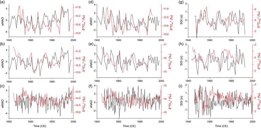
B. R. Schöne et al.: Freshwater pearl mussels as long-term, high-resolution stream water isotope recorders                     675

lecting additional specimens that could have covered the time       tion of the outer shell layer (iOSL, consisting of nacrous mi-
interval between the initial collection and the preparation of      crostructure) perpendicularly to the previous annual growth
this paper; instead, we relied on bivalves that we obtained –       line (Fig. 2c). Annual increment width chronologies were
with permission – for a co-author’s (AEM, formerly known            detrended with stiff cubic spline functions and standardized
as Elena Dunca) postdoctoral project and another co-author’s        to produce dimensionless measures of growth (standardized
(SMB) doctoral thesis.                                              growth indices, i.e., SGI values – σ ) following standard scle-
   The bedrock in the catchments studied is dominated by            rochronological methods (Helama et al., 2006; Butler et al.,
orthogneiss and granodiorite. The vegetation at GTB (ca.            2013; Schöne, 2013). Briefly, for detrending, measured an-
90 m a.s.l., above sea level) and GJ (ca. 200 m a.s.l.) consisted   nual increment widths were divided by the data predicted by
of a mixed birch forest, whereas conifers, shrubs and bushes        the cubic spline fit. From each resulting growth index, we
dominated at NJB (ca. 400 m a.s.l.). Thus, the streams stud-        subtracted the mean of all growth indices and divided the
ied were rich in humin acids. The streams studied were fed          result by the standard deviation of all of the growth indices
by small upstream open (flow-through) lakes.                        of the respective bivalve specimen. This transformation re-
                                                                    sulted in SGI chronologies. Due to low heteroscedasticity,
2.1   Sample preparation                                            no variance correction was needed (Frank et al., 2007). Un-
                                                                    certainties in annual increment measurements resulted in a
The soft tissues were removed immediately after collection          SGI error of ±0.06σ .
and shells were then air-dried. One valve of each specimen
was wrapped in a protective layer of WIKO metal epoxy               2.3   Stable isotope analysis
resin no. 5 and mounted to a Plexiglas cube using Gluetec
Multipower plastic welder no. 3. Shells were then cut perpen-       The other polished shell slab of each specimen was used
dicular to the growth lines using a low-speed saw (Buehler          for stable isotope analysis. To avoid contamination of the
Isomet) equipped with a diamond-coated (low-diamond con-            shell aragonite powders (Schöne et al., 2017), the cured
centration) wafering thin blade (400 µm thickness). One             epoxy resin and the periostracum were completely removed
specimen (ED-NJB-A3R) was cut along the longest axis,               prior to sampling. A total of 1551 powder samples (32–
whereas all of the others were cut along the height axis            128 µg) were obtained from the oOSL by means of mi-
from the umbo to the ventral margin (Fig. 2a). From each            cromilling (Fig. 2c) under a stereomicroscope at 160× mag-
specimen, two ca. 3 mm thick shell slabs were obtained and          nification. An equidistant sampling strategy was applied, i.e.,
mounted onto glass slides with the mirroring sides (the por-        the milling step size was held constant within each annual
tions that were located to the left and right of the saw blade      increment (Schöne et al., 2005c). We used a cylindrical,
during the cutting process) facing upward. This method fa-          diamond-coated drill bit (1 mm diameter; Komet/Gebr. Bras-
cilitated the temporal alignment of isotope data measured in        seler GmbH and Co. KG, model no. 835 104 010) mounted
one slab to growth patterns determined in the other shell slab.     on a Rexim Minimo drill. While the drilling device was af-
The shell slabs were ground on glass plates using suspen-           fixed to the microscope, the sample was handheld during
sions of 800 and 1200 grit SiC powder and subsequently pol-         sampling. In early ontogenetic years, up to 16 samples were
ished with Al2 O3 powder (grain size of 1 µm) on a Buehler          obtained between successive annual growth lines. In the lat-
G-cloth. Between each grinding step and after polishing, the        est ontogenetic portions of specimens ED-NJB-A2R (the last
shell slabs were ultrasonically cleaned with water.                 year of life) and ED-GJ-D6R (the last 9 years of life), each
                                                                    isotope sample represented 2–3 years.
2.2   Shell growth pattern analysis                                    Stable carbon and oxygen isotopes were measured at the
                                                                    Institute of Geosciences at the J.W. Goethe University of
For growth pattern analysis, one polished shell slab was im-        Frankfurt/Main (Germany). Carbonate powder samples were
mersed in Mutvei’s solution for 20 min at 37–40 ◦ C under           digested in He-flushed borosilicate Exetainer vials at 72 ◦ C
constant stirring (Schöne et al., 2005b). After careful rins-       using a water-free phosphoric acid. The released CO2 gas
ing in demineralized water, the stained sections were air-          was then measured in continuous-flow mode with a Ther-
dried under a fume hood. Dyed thick-sections were then              moFisher MAT 253 gas source isotope ratio mass spectrom-
viewed under a binocular microscope (Olympus SZX16) that            eter coupled to a GasBench II. Stable isotope ratios were cor-
was equipped with sectoral dark-field illumination (Schott          rected against an NBS-19 calibrated Carrara marble (δ 13 C =
VisiLED MC1000) and were photographed using a Canon                 +2.02 ‰; δ 18 O = −1.76 ‰). Results are expressed as parts
EOS 600D camera (Fig. 2b). The widths of the annual incre-          per thousand (‰) relative to the Vienna Pee Dee Belem-
ments were determined to the nearest ca. 1 µm with image            nite (VPDB) scale. The long-term accuracy based on blindly
processing software (Panopea, © Peinl and Schöne). Mea-             measured reference materials with known isotope compo-
surements were completed in the outer portion of the outer          sition is better than 0.05 ‰ for both isotope systems. Note
shell layer (oOSL, consisting of prismatic microstructure)          that no correction was applied for differences in fractionation
from the boundary between the oOSL and the inner por-               factors of the reference material (calcite) and shells (arag-

www.hydrol-earth-syst-sci.net/24/673/2020/                                         Hydrol. Earth Syst. Sci., 24, 673–696, 2020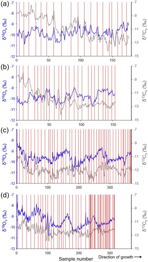
676            B. R. Schöne et al.: Freshwater pearl mussels as long-term, high-resolution stream water isotope recorders

Figure 1. Maps showing the sample sites in northern Sweden. (a) Topographic map of Scandinavia. (b) An enlargement of the red box
in panel (a) showing Norrbotten County (yellow), a province in northern Sweden, and localities where bivalve shells (Margaritifera mar-
garitifera) were collected and isotopes in rivers and precipitation were measured. The shell collection sites (filled circles) are coded as
follows: NJB represents the Nuortejaurbäcken, GTB represents the Grundträsktjärnbäcken and GJ represents Görjeån River. Sk represents
the Skellefte River (near Slagnäs), a GNIR site. The GNIP sites of Racksund and Arjeplog are represented by Rs and Ap, respectively.
The base map in panel (a) is sourced from TUBS and used under a Creative Commons license: https://commons.wikimedia.org/wiki/File:
Sweden_in_Europe_(relief).svg (last access: 5 February 2020). The base map in panel (b) is sourced from Erik Frohne (redrawn by Sil-
verkey) and used under a Creative Commons license: https://commons.wikimedia.org/wiki/File:Sweden_Norrbotten_location_map.svg (last
access: 5 February 2020).

Table 1. Shell of M. margaritifera from three streams in northern Sweden used in the present study for isotope and growth pattern analysis.
The last hyphenated section of the specimen ID represents whether bivalves were collected alive (A) or dead (D), the specimen number and
which valve was used (R denotes right and L denotes left).

        Stream name                      Specimen ID           Coordinates and              Agea       Alive during years (CE)           No. isotope samples
                                                               elevation                  (years)                         (CE)           (coverage of yearsc )
        Nuortejaurbäcken                 ED-NJB-A6R            65◦ 420 13.2200 N,              22                      1972–1993                  175 (1–22b )
                                         ED-NJB-A4R            019◦ 020 31.0100 E,             27                      1967–1993                  154 (2–27b )
                                         ED-NJB-A2R            ca. 400 m a.s.l.                48                      1946–1993                   78 (2–48b )
                                         ED-NJB-A3R                                            24                      1970–1993                   50 (1–24b )
        Grundträsktjärnbäcken            ED-GTB-A1R            66◦ 020 59.9800 N,              51                      1943–1993                   368 (2–49)
                                         ED-GTB-A2R            022◦ 050 02.2500 E,             51                      1943–1993                   315 (3–49)
                                                               ca. 90 m a.s.l.
        Görjeån                          ED-GJ-A1L             66◦ 200 30.7700 N,              80                      1916–1997                  56 (25–80b )
                                         ED-GJ-A2R             020◦ 300 15.0200 E,             82                      1918–1997                    76 (1–78)
                                         ED-GJ-A3L             ca. 200 m a.s.l.               123                      1875–1997                 110 (29–122)
                                         ED-GJ-D5L                                            181                      1819–1999                  169 (1–180)
      a Minimum estimate of life span. b Last sampled year incomplete. c Add 10 years to these values to obtain approximate ontogenetic years.

Hydrol. Earth Syst. Sci., 24, 673–696, 2020                                                                  www.hydrol-earth-syst-sci.net/24/673/2020/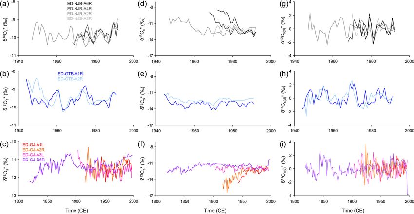
B. R. Schöne et al.: Freshwater pearl mussels as long-term, high-resolution stream water isotope recorders                             677

Figure 2. Sclerochronological analysis of Margaritifera margaritifera. (a) The left valve of a freshwater pearl mussel. The cutting axis is
indicated by a white line. Note the erosion in the umbonal shell portion. (b) A Mutvei-immersed shell slab showing the outer and inner shell
layers (OSL and ISL, respectively) separated by the myostracum (white line). The OSL is further subdivided into an outer and inner portion
(oOSL and iOSL, respectively). The ISL and iOSL consist of a nacreous microstructure, and the oOSL consists of a prismatic microstructure.
(c) An enlargement of panel (b) shows the annual growth patterns. The annual increment width measurements (yellow) were completed as
perpendiculars from the intersection of the oOSL and iOSL toward the next annual growth line. The semitransparent red and orange boxes
schematically illustrate the micromilling sampling technique.

onite; verified by Raman spectroscopy), because the pale-               https://www.smhi.se (last access: 5 February 2020). From
othermometry equation used below (Eq. 2) also did not con-              these data, the monthly stream water temperature (Tw ) was
sider these differences (Füllenbach et al., 2015). However,             computed using the summer air–stream water temperature
the correction of −0.38 ‰ would be required if δ 18 O val-              conversion by Schöne et al. (2004a) and was supplemented
ues of shells and other carbonates were compared with each              by the standard errors of the slope and intercept:
other.
                                                                        Tw = 0.88 ± 0.05 × Ta − 0.86 ± 0.49.                            (1)
2.4   Instrumental data sets                                            2.5    Weighted annual shell isotope data

Shell growth and isotope data were compared to a set of                 Because the shell growth rate varied during the growing sea-
environmental variables including the station-based winter              son – with the fastest biomineralization rates occurring dur-
(DJFM) NAO index (obtained from https://climatedataguide.               ing June and July (Dunca et al., 2005) – the annual growth
ucar.edu, last access: 9 April 2019) as well as oxygen iso-             increments are biased toward summer, and powder samples
tope values of river water (δ 18 Ow ) and weighted (corrected           taken from the shells at equidistant intervals represent dif-
for precipitation amounts) oxygen isotope values of precip-             ferent amounts of time. To compute growing season av-
itation (δ 18 Op ). Data on monthly river water and precipita-          erages (henceforth referred to as “annual averages”) from
tion were sourced from the Global Network of Isotopes in                such intra-annual shell isotope data (δ 18 Os , δ 13 Cs ), weighted
Precipitation (GNIP) and the Global Network of Isotopes                 (henceforth denoted with an asterisk) annual means are thus
in Rivers (GNIR), available at the International Atomic En-             needed, i.e., δ 18 O∗s and δ 13 C∗s values (Schöne et al., 2004a).
ergy Agency:https://nucleus.iaea.org/wiser/index.aspx (last             The relative proportion of time of the growing season rep-
access: 1 April 2019). Furthermore, monthly air temperature             resented by each isotope sample was computed from a pre-
(Ta ) data came from the station Stensele, and are available            viously published intra-annual growth curve of juvenile M.
at the Swedish Meteorological and Hydrological Institute:               margaritifera from Sweden (Dunca et al., 2005). For exam-

www.hydrol-earth-syst-sci.net/24/673/2020/                                               Hydrol. Earth Syst. Sci., 24, 673–696, 2020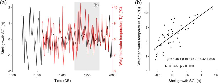
678             B. R. Schöne et al.: Freshwater pearl mussels as long-term, high-resolution stream water isotope recorders

ple, if four isotope samples were taken between two winter           revised (shell growth vs. temperature) model is as follows:
lines at equidistant intervals, the first sample would represent
22.38 % of the time of the main growing season duration,             Tw∗ = 1.45 ± 0.19 × SGI + 8.42 ± 0.08.                      (3)
and the second, third and fourth would represent 20.28 %,
24.47 % and 32.87 % of the time of the main growing sea-             For coherency purposes, we also applied this model to post-
son, respectively (Table 2). Accordingly, the weighted annual        1859 SGI values and computed stream water temperatures
mean isotope values (δ 18 O∗s , δ 13 C∗s ) were calculated by mul-   that were subsequently used to estimate δ 18 O∗wr(SGI) values.
tiplying these numbers (weights) by the respective δ 18 Os and          To assess how well the shells recorded δ 18 Ow values at
δ 13 Cs values and dividing the sum of the products by 100 (see      intra-annual timescales, we focused on two shells from NJB
Supplement). The four isotope samples from the example               (ED-NJB-A4R and ED-NJB-A6R), which provided the high-
above comprise the time intervals from 23 May to 22 June,            est isotope resolution of 1–2 weeks per sample during the few
23 June to 21 July, 22 July to 25 August, and 26 August              years of overlap between the GNIP and GNIR data. Note that
to 12 October, respectively. Missing isotope data due to lost        (only for this bivalve sampling locality) monthly instrumen-
powder, machine error, air in the Exetainer etc. were filled in      tal oxygen isotope data were available from the GNIP and
using linear interpolation in 20 instances. We assumed that          GNIR data sets (data by Burgman et al., 1981). The δ 18 Ow
the timing and rate of seasonal growth remained nearly un-           data were measured in the Skellefte River near Slagnäs, ca.
changed throughout the lifetime of the specimens and in the          40 km SW of NJB (65◦ 340 59.5000 N, 018◦ 100 39.1200 E) and
study region (see also Sect. 4).                                     covered the time interval from 1973 to 1980. The δ 18 Op data
                                                                     came from Racksund (66◦ 020 60.0000 N, 017◦ 370 60.0000 E; ca.
2.6   Reconstruction of oxygen isotope signatures of                 75 km NW of NJB) and covered the time interval from 1975
      stream water on annual and intra-annual                        to 1979. Because precipitation amounts were not available
      timescales                                                     from Racksund, we computed average monthly precipitation
                                                                     amounts from data recorded at Arjeplog (66◦ 020 60.0000 N,
To assess how well the shells recorded δ 18 Ow values on
                                                                     017◦ 530 60.0000 E) from 1961 to 1967 (see Supplement). Ar-
inter-annual timescales, the stable oxygen isotope signature
                                                                     jeplog is located ca. 65 km NW of NJB and ca. 12 km W of
of stream water (δ 18 O∗wr ) during the main growing season
                                                                     Racksund. Equation (2) was used to calculate δ 18 O∗wr values
(“annual” δ 18 O∗wr ) was reconstructed from δ 18 O∗s data and
                                                                     from individual δ 18 O∗s data and water temperature that ex-
the arithmetic average of (monthly) stream water temper-
                                                                     isted during the time when the respective shell portion was
atures, Tw , during the same time interval, i.e., 23 May–
                                                                     formed. Intra-annual water temperatures were computed as
12 October. Using this approach, the effect of temperature-
                                                                     weighted averages, Tw∗ , from monthly Tw considering sea-
dependent oxygen isotope fractionation was removed from
                                                                     sonal changes in the shell growth rate. For example, if four
the δ 18 O∗s data. For this purpose, the paleothermometry equa-
                                                                     powder samples were taken from the shell at equidistant in-
tion of Grossman and Ku (1986; corrected for the VPDB–
                                                                     tervals within one annual increment, 6.29 % of the first sam-
VSMOW scale difference following Gonfiantini et al., 1995)
                                                                     ple was formed in May and 18.63 % was formed in June (sum
was solved for δ 18 O∗wr , Eq. (2):
                                                                     ca. 25 %). The average temperature during that time interval
              19.43 − 4.34 × δ 18 O∗s − Tw                           is computed using these numbers as follows: (Tw of May ×
δ 18 O∗wr =                                .                  (2)    0.0629 + Tw of June × 0.1863)/25. A total of 6.86 % of the
                        −4.34
                                                                     second sample from that annual increment formed in June
Because air temperature data were only available from 1860           and 17.97 % formed in July. Accordingly, the average tem-
onward, Tw values prior to that time were inferred from age-         perature was (Tw of June ×0.0686+Tw of July ×17.47)/25.
detrended and standardized annual growth increment data              Note that annual δ 18 O∗wr values can also be computed from
(SGI values) using a linear regression model similar to that         intra-annual δ 18 O∗wr data, but this approach is much more
introduced by Schöne et al. (2004a). In the revised model,           time-consuming and complex than the method described fur-
SGI data of 25 shells from northern Sweden (15 published             ther above. However, both methods produce nearly identical
chronologies, provided in the article cited above, and 10 new        results (see Supplement).
chronologies from the specimens studied in the present pa-
per) were arithmetically averaged for each year and then re-         2.7   Stable carbon isotopes of the shells
gressed against weighted annual water temperature, hereafter
referred to as annual Tw∗ . The annual Tw∗ data consider vari-       Besides the winter and summer NAO index, weighted an-
ations in the seasonal shell growth rate. A total of 6.29 %,         nual stable carbon isotope data of the shells, δ 13 C∗s values,
25.49 %, 24.52 %, 21.92 %, 16.88 % and 4.90 % of the an-             were compared to shell growth data (SGI chronologies). Be-
nual growth increment was formed in each month between               cause the δ 13 C∗s values could potentially be influenced by on-
May and October, respectively. The values were multiplied            togenetic effects, the chronologies were detrended and stan-
by Tw of the corresponding month and the sum of the prod-            dardized (δ 13 C∗s(d) ) following methods typically used to re-
ucts was divided by 100 to obtain the annual Tw∗ data. The           move ontogenetic age trends from annual increment width

Hydrol. Earth Syst. Sci., 24, 673–696, 2020                                         www.hydrol-earth-syst-sci.net/24/673/2020/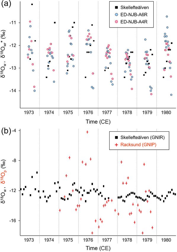
B. R. Schöne et al.: Freshwater pearl mussels as long-term, high-resolution stream water isotope recorders                                                    679

Table 2. Weights for isotope samples of Margaritifera margaritifera. Due to variations in the seasonal shell growth rate, each isotope sample
taken at equidistant intervals represents different amounts of time. To calculate seasonal or annual averages from individual isotope data, the
relative proportion of time of the growing season contained in each sample must be considered when weighted averages are computed. The
duration of the growing season comprises 143 d and covers the time interval from 23 May to 12 October.

    Number of isotope               Weight of nth isotope sample (%) within an annual increment; direction of growth to the right (increasing numbers)
    samples per annual      1st    2nd      3rd      4th      5th      6th     7th      8th      9th     10th     11th    12th     13th     14th     15th    16th
    increment
    1                    100.00
    2                     42.66   57.34
    3                     27.97   31.47   40.56
    4                     22.38   20.28   24.47    32.87
    5                     18.18   15.39   18.88    20.27   27.28
    6                     15.38   12.59   14.69    16.78   18.18    22.38
    7                     13.29   11.88   11.19    13.29   13.99    16.08    20.28
    8                     11.59   10.79    9.09    11.19   12.58    11.89    14.69    18.18
    9                     10.49    9.79    7.69     9.09   10.49    11.89    10.49    13.29    16.78
    10                     9.79    8.39    7.69     7.70    9.09     9.78     9.80    10.49    11.89    15.38
    11                     9.09    7.69    7.70     5.59    7.69     8.39     9.79     8.40    10.49    10.48   14.69
    12                     8.39    6.99    7.00     5.59    6.99     7.70     8.39     8.39     7.69    10.49    9.09    13.29
    13                     7.69    6.30    6.99     5.59    5.60     6.29     7.69     8.40     6.99     7.69    9.79     8.39    12.59
    14                     7.69    5.60    6.29     5.59    4.90     6.29     6.30     6.99     6.99     7.70    6.28     9.10     8.39    11.89
    15                     6.29    6.30    5.59     5.60    4.19     5.60     5.59     6.99     6.30     6.99    6.29     7.00     8.38     7.70    11.19
    16                     6.29    5.60    5.59     4.90    4.19     4.90     5.59     5.60     6.29     4.90    7.69     5.59     7.70     6.99     7.69   10.49

chronologies (see, e.g., Schöne, 2013). Detrending was car-                          values were similar to the previously published coefficient
ried out with cubic spline functions capable of removing any                         of determination for a stacked record using M. margaritifera
directed trend toward higher or lower values throughout the                          specimens from streams across Sweden (R 2 = 0.60; Schöne
lifetime.                                                                            et al., 2005a; note that this number is for SGI vs. an arith-
                                                                                     metic annual Tw ; a regression of SGI against weighted an-
                                                                                     nual Tw returns an R 2 of 0.64).
3        Results
                                                                                     3.2      Shell stable oxygen isotope data
The lengths of the annual increment chronologies of M. mar-
garitifera from the three streams studied (the Nuortejaur-                           The shell oxygen isotope curves showed distinct seasonal
bäcken, Grundträsktjärnbäcken and Görjeån) ranged from                               and inter-annual variations (Figs. 4, 5). The former were par-
21 to 181 years and covered the time interval from 1819                              ticularly well developed in specimens from GTB and NJB
to 1999 CE (Table 1). Because the umbonal shell portions                             (Fig. 4), which were sampled with a very high spatial resolu-
were deeply corroded and the outer shell layer was missing                           tion of ca. 30 µm (ED-GTB-A1R, ED-GTB-A2R, ED-NJB-
– a typical feature of long-lived freshwater bivalves (Schöne                        A4R and ED-NJB-A6R). In these shells, up to 16 samples
et al., 2004a; Fig. 2a) – the actual ontogenetic ages of the                         were obtained from single annual increments translating into
specimens could not be determined and may have been up to                            a temporal resolution of 1–2 weeks per sample. Typically,
10 years higher than the ages listed in Table 1.                                     the highest δ 18 Os values of each cycle occurred at the winter
                                                                                     lines, and the lowest values occurred about half way between
3.1       Shell growth and temperature                                               consecutive winter lines (Fig. 4). The largest seasonal δ 18 Os
                                                                                     amplitudes of ca. 2.20 ‰ were measured in specimens from
The 10 new SGI series from NJB, GTB and GJ were com-                                 GTB (−8.68 ‰ to −10.91 ‰), and ca. 1.70 ‰ was measured
bined with 15 published annual increment series of M. mar-                           in shells from NJB (−8.63 ‰ to −10.31 ‰).
garitifera from the Pärlälven, Pärlskalsbäcken and Böls-                                Weighted annual shell oxygen isotope (δ 18 O∗s ) values fluc-
manån streams (Schöne et al., 2004a, b, 2005a) to form a                             tuated on decadal timescales (common period of ca. 8 years)
revised Norrland master chronology. During the 50-year cal-                          with amplitudes larger than those occurring on seasonal
ibration interval from 1926 to 1975 (the same time interval                          scales, i.e., ca. 2.50 ‰ and 3.00 ‰ in shells from NJB
was used in the previous study by Schöne et al., 2004a, b,                           (−8.63 ‰ to −11.10 ‰) and GTB (−7.84 ‰ to −10.85 ‰),
2005a), the chronology was significantly (p < 0.05; note,                            respectively (Fig. 5a, b). The chronologies from GJ also re-
all p values of linear regression analyses in this paper are                         vealed a century-scale variation with minima in the 1820s
Bonferroni-adjusted) and positively correlated (R = 0.74;                            and 1960s and maxima in the 1880s and 1990s (Fig. 5c). The
R 2 = 0.55) with the weighted annual stream water temper-                            δ 18 O∗s curves of specimens from the same locality showed
ature (Tw∗ ) during the main growing season (Fig. 3). These                          notable agreement in terms of absolute values and visual

www.hydrol-earth-syst-sci.net/24/673/2020/                                                               Hydrol. Earth Syst. Sci., 24, 673–696, 2020
680 B. R. Schöne et al.: Freshwater pearl mussels as long-term, high-resolution stream water isotope recorders
Figure 3. (a) Time series and (b) cross-plot of the age-detrended and standardized annual shell growth rate (SGI values) and water temper-
ature during the main growing season (23 May–12 October). Water temperatures were computed from monthly air temperature data using a
published transfer function and considering seasonally varying rates of shell growth. The gray box in panel (a) denotes the 50-year calibration
interval from which the temperature model (b) was constructed. As seen from the cross-plot in panel (b), 55 % of the variation in annual
shell growth was highly significantly explained by water temperature. Higher temperature resulted in faster shell growth.
agreement (running similarity), specifically specimens from cording to nonparametric t tests, these data sets are statisti-
NJB and GTB (Fig. 5a, b). However, the longest chronology cally indistinguishable. Furthermore, the inter-annual trends
from GJ only showed slight agreement with the remaining of δ 18 O∗wr and δ 18 Ow values were similar (Fig. 6a): val-
three series from that site (Fig. 5c). The similarity among ues declined by ca. 1.00 ‰ between 1973 and 1977 fol-
the series also changed through time (Fig. 5a, b ,c). In some lowed by a slight increase of ca. 0.50 ‰ until 1980. In con-
years, the difference between the series was less than 0.20 ‰ trast to the damped stream water signal (the average sea-
at NJB (N = 4) and GTB (N = 2; 1983) and 0.10 ‰ at GJ sonal range during the 4 years – 1975, 1976, 1978, and
(N = 4; 1953), whereas, in other years, the differences varied 1979 – for which both stream water and precipitation data
by up to 0.82 ‰ at NJB and 1.00 ‰ at GTB and GJ. Average were available was −1.50 ± 0.57 ‰), δ 18 Op values exhibited
shell oxygen isotope chronologies of the three streams stud- much stronger fluctuations at the seasonal scale (on aver-
ied exhibited a strong running similarity (passed the “Gleich- age, −9.37 ± 2.81 ‰; extreme monthly values of −4.21 ‰
läufigkeitstest” by Baillie and Pilcher, 1973, for p < 0.001) and −17.60 ‰; N = 46; station Racksund; Fig. 6b) and
and were significantly positively correlated with each other on inter-annual timescales (unweighted annual averages of
(the R 2 value of NJB vs. GTB was 0.34, NJB vs. GJ was −11.41 ‰ to 13.68 ‰; weighted December–September av-
0.40 and GTB vs. GJ was 0.36 – all at p < 0.0001). erages of −9.54 ‰ to 13.16 ‰).
Despite the limited number of instrumental data, season-
3.3 Shell stable oxygen isotope data and instrumental ally averaged δ 18 O∗wr data showed some – although not al-
records ways statistically significant – agreement with δ 18 Ow and
weighted δ 18 Op data (corrected for precipitation amounts),
At NJB – the only bivalve sampling site for which measured respectively, both in terms of correlation coefficients and ab-
stream water isotope data were available from nearby locali- solute values (Table 3). These findings were corroborated by
ties – the May–October ranges of reconstructed and instru- the regression analyses of instrumental δ 18 Op values against
mental stream water δ 18 O values between 1973 and 1980 δ 18 Ow values (Table 3). For example, the oxygen isotope val-
(excluding 1977 due to missing δ 18 Ow data) were in close ues of summer (June–September) precipitation were signif-
agreement (shells were 2.83 and 3.19 ‰ vs. stream water icantly (Bonferroni-adjusted p < 0.05) and positively corre-
which was 3.20 ‰; Fig. 6a). During the same time interval, lated with those of shell carbonate precipitated during the
arithmetic means ± 1 standard deviation of the shells were same time interval (98 % of the variability was explained
−12.48 ± 0.74 ‰ (ED-NJB-A6R; N = 79) and −12.45 ± in both specimens, but only at p < 0.05 in ED-NJB-A6R).
0.66 ‰ (ED-NJB-A4R; N = 44), whereas the stream water Likewise, δ 18 Ow and δ 18 Op values during summer were
value was −12.33±0.76 ‰ (Skellefte River; N = 42). When positively correlated with each other (R = 0.91), although
computed from growing season averages (N = 7), shell val- less significantly (p = 0.546). Strong relationships were
ues were −12.48 ± 0.29 ‰ and −12.42 ± 0.34 ‰, respec- also found for δ 18 O∗wr and δ 18 Ow values during the main
tively, and the stream water value was −12.30±0.32 ‰. Ac- growing season as well as annual δ 18 O∗wr and December–
Hydrol. Earth Syst. Sci., 24, 673–696, 2020 www.hydrol-earth-syst-sci.net/24/673/2020/B. R. Schöne et al.: Freshwater pearl mussels as long-term, high-resolution stream water isotope recorders 681
Table 3. Relationship between the stable oxygen isotope values in precipitation (amount-corrected δ 18 Op ), river water and shells of Margar-
itifera margaritifera from Nuortejaurbäcken during different portions of the year (during the 4 years for which data from shells, water and
precipitation were available: 1975, 1976, 1978, and 1979; hence N = 4). The arithmetic mean δ 18 O values for each portion of the year are
also given. The rationale behind the comparison of δ 18 O values of winter precipitation and spring (May–June) river water or shell carbonate
is that the isotope signature of meltwater may have left a signal in the water. Statistically significant values (Bonferroni-adjusted p < 0.05)
are marked in bold. Isotope values next to months represent multiyear averages.
δ 18 Op (Racksund) δ 18 Ow (Skellefte River)
Season Dect−1 to Sept Jun to Sep Dect−1 to Febt May to Oct Jun to Sep May to June
−11.39 ‰ −10.98 ‰ −14.18 ‰ −12.46 ‰ −12.39 ‰ −13.08 ‰
δ 18 Ow May–Oct R = 1.00
Skellefte River −12.46 ‰ R 2 = 1.00
p = 0.006
Jun–Sep R = 0.91
−12.39 ‰ R 2 = 0.83
p = 0.546
May–Jun R = 0.95
−13.08 ‰ R 2 = 0.90
p = 1.000
δ 18 O∗wr May–Oct R = 0.98 R = 0.99
ED-NJB-A6R −12.57 ‰ R 2 = 0.96 R 2 = 0.97
p = 0.134 p = 0.065
Jun–Sep R = 0.99 R = 0.86
−12.44 ‰ R 2 = 0.98 R 2 = 0.75
p = 0.045 p = 0.609
May–Jun R = 0.46 R = 0.64
−12.44 ‰ R 2 = 0.21 R 2 = 0.41
p = 1.000 p = 1.000
δ 18 O∗wr May–Oct R = 0.99 R = 0.99
ED-NJB-A4R −12.46 ‰ R 2 = 0.98 R 2 = 0.98
p = 0.035 p = 0.034
Jun–Sep R = 0.99 R = 0.95
−12.43 ‰ R 2 = 0.98 R 2 = 0.91
p = 0.070 p = 0.217
May–Jun R = 0.76 R = 0.89
−12.30 ‰ R 2 = 0.58 R 2 = 0.80
p = 1.000 p = 0.484
September δ 18 Op values. The underlying assumption for the δ 18 O∗wr of −12.57 ‰ and −12.46 ‰) and during summer
latter was that the δ 18 O∗wr average value reflects the com- (δ 18 Ow of −12.39 ‰; δ 18 O∗wr of −12.44 ‰ and −12.43 ‰)
bined δ 18 Op of snow precipitated during the last winter (re- (Table 3). In contrast, isotopes in precipitation and river wa-
ceived as meltwater during spring) and rain precipitated dur- ter showed larger discrepancies (see the text above, Fig. 6b
ing summer. Instrumental data supported this hypothesis, be- and Table 3).
cause stream water δ 18 O values during the main growing
season were highly significantly and positively correlated 3.4 Shell stable oxygen isotope data and synoptic
with December–September δ 18 Op data (Table 3). Conversely, circulation patterns (NAO)
changes in the isotope signal of winter (December–February)
snow were only weakly and not significantly mirrored by Site-specific annual δ 18 O∗wr (and δ 18 O∗wr(SGI) ) chronolo-
changes in stream water oxygen isotope values during the gies (computed as arithmetic averages of all chronologies
snowmelt period (May–June) or in δ 18 O∗wr values from shell at a given stream) were significantly (Bonferroni-adjusted
portions formed during the same time interval (Table 3). Dur- p < 0.05) positively correlated with the NAO indices (Fig. 7,
ing the 4 years under study (1975, 1976, 1978 and 1979), Table 4). In NAO+ years, the δ 18 O∗wr (and δ 18 O∗wr(SGI) ) val-
measured and reconstructed δ 18 Ow values were nearly iden- ues were higher than during NAO− years. The strongest cor-
tical during the main growing season (δ 18 Ow of −12.46 ‰; relation existed between the winter (December–March) NAO
www.hydrol-earth-syst-sci.net/24/673/2020/ Hydrol. Earth Syst. Sci., 24, 673–696, 2020682 B. R. Schöne et al.: Freshwater pearl mussels as long-term, high-resolution stream water isotope recorders
(wNAO) index. Between 1947 and 1991 (the time interval for
which isotope data were available for all sites), the R 2 val-
ues were more similar to each other and ranged between 0.27
and 0.46 (Table 4). All sites reflected well-known features of
the instrumental NAO index series such as the recent (1970–
2000) positive shift toward a more dominant wNAO, which
delivered isotopically more positive (less depleted in 18 O)
winter precipitation to our region of interest (Fig. 7a, b, c).
The correlation between δ 18 O∗wr (and δ 18 O∗wr(SGI) ) values and
the summer (June–August) NAO index was much lower than
for the wNAO, but likewise positive and sometimes signifi-
cant at p < 0.05 (Table 4). Between 1947 and 1991, 7 % to
43 % of the inter-annual oxygen isotope variability was ex-
plained by the summer NAO index.
We have also computed an average δ 18 O∗wr(SGI) curve for
the entire study region (Fig. 8a, b, c). Because the level
(absolute values) of the three streams differed from each
other (average δ 18 O∗wr values of NJB, GTB and GJ from
1947 to 1992 were −12.51 ‰, −12.21 ‰ and −14.16 ‰,
respectively), the site-specific series were standardized and
then arithmetically averaged. The resulting chronology,
δ 18 O∗wr(Norrland) , was strongly positively and statistically sig-
nificantly (Bonferroni-adjusted p value below 0.05) corre-
lated with the wNAO index (56 % of the variability ex-
plained; Fig. 8a). Despite the limited instrumental data set,
δ 18 O values of river water and precipitation were strongly
positively correlated with the wNAO index (R 2 values of
0.72 and 0.84, respectively; Fig. 8d, e), but the Bonferroni-
adjusted p values exceeded 0.05 (note, the uncorrected p val-
ues were 0.07 and 0.03, respectively).
3.5 Shell stable carbon isotope data
Shell stable carbon isotope (δ 13 Cs ) data showed less distinct
seasonal variations than δ 18 Os values, but the highest values
Figure 4. Shell stable oxygen and carbon isotope chronologies
from four specimens of Margaritifera margaritifera from Nuorte-
were also often associated with the winter lines and the low-
jaurbäcken and Grundträsktjärnbäcken that were sampled with very est values occurred between subsequent winter lines (Fig. 4).
high spatial resolution and from which the majority of the isotope The largest seasonal amplitudes of ca. 3.90 ‰ were observed
data were obtained (Table 1): (a) ED-NJB-A6R, (b) ED-NJB-A4R, in specimens from NJB (−8.21 ‰ to −12.10 ‰) and ca. 1 ‰
(c) ED-GTB-A1R and (d) ED-GTB-A2R. Individual isotope sam- smaller ranges at GTB (−10.97 ‰ to −13.88 ‰).
ples represent time intervals of a little as 6 d to 2 weeks in ontoge- Weighted annual δ 13 C∗s curves varied greatly from each
netically young shell portions and up to one full growing season in other in terms of change throughout the lifetime of the
the last few years of life. Red vertical lines represent annual growth organism, among localities and even at the same locality
lines. Because the umbonal shell portions are corroded, the exact (Fig. 5d, e, f). Note that all curves started in early ontogeny
ontogenetic age at which the chronologies start cannot be provided. (below the age of 10), except for ED-GJ-A1L and ED-GJ-
Assuming that the first 10 years of life are missing, sampling in
A3L that began at a minimum age of 25 and 29, respectively
panel (a) started in year 11, in panels (b) and (c) in year 12, and in
panel (d) in year 13 (see also Table 1).
(Table 1). Whereas two specimens from NJB (ED-NJB-
A6R and ED-NJB-A4R) showed strong ontogenetic δ 13 C∗s
trends from ca. −8.70 ‰ to −12.50 ‰, weaker trends to-
ward more negative values were observed in ED-NJB-A2R
and δ 18 O∗wr (and δ 18 O∗wr(SGI) ) values at NJB (44 % to 49 % (ca. −10.00 ‰ to −11.70 ‰) and shells from GTB (ca.
of the variability is explained). At GTB, the amount of vari- −11.50 ‰ to −13.00 ‰). Opposite ontogenetic trends oc-
ability explained ranged between 24 % and 27 %, whereas curred in ED-GJ-A1L and ED-GJ-A2R (ca. −15.00 ‰ to
at GJ only 16 % to 18 % of the inter-annual δ 18 O∗wr (and −12.00 ‰), but no trends at all were found in ED-NJB-
δ 18 O∗wr(SGI) ) variability was explained by the winter NAO A3R, ED-GJ-A3L and ED-GJ-D6R (fluctuations around
Hydrol. Earth Syst. Sci., 24, 673–696, 2020 www.hydrol-earth-syst-sci.net/24/673/2020/B. R. Schöne et al.: Freshwater pearl mussels as long-term, high-resolution stream water isotope recorders 683
Figure 5. Annual shell stable oxygen and carbon isotope chronologies of the specimens of Margaritifera margaritifera studied. Data were
computed as weighted averages from intra-annual isotope data, i.e., growth rate-related variations were taken into consideration. Panels
(a), (d) and (g) represent the stream Nuortejaurbäcken; panels (b), (e) and (h) represent the stream Grundträsktjärnbäcken; and panels (c), (f)
and (i) represent Görjeån River. (a–c) Oxygen isotopes, (d–f) carbon isotopes, and (g–i) detrended and standardized carbon isotope values
are also shown.
Table 4. Site-specific annual isotope chronologies of Margaritifera margaritifera shells linearly regressed against winter and summer NAO
(wNAO and sNAO, respectively) as well as the detrended and standardized shell growth rate (SGI). δ 18 O∗wr data were computed from shell
oxygen isotope data and temperature data were computed from instrumental air temperatures, whereas, in the case of δ 18 O∗wr(SGI) data,
temperatures were estimated from a growth-temperature model. See text for details. Statistically significant values (Bonferroni-adjusted
p < 0.05) are marked in bold.
δ 18 O∗wr δ 18 O∗wr(SGI) δ 13 C∗s(d)
NJB GTB GJ NJB GTB GJ NJB GTB GJ
wNAO R = 0.67 R = 0.49 R = 0.39 R = 0.70 R = 0.52 R = 0.42 R = −0.18 R = −0.31 R = −0.10
(DJFM) R 2 = 0.44 R 2 = 0.24 R 2 = 0.16 R 2 = 0.49 R 2 = 0.27 R 2 = 0.18 R 2 = 0.03 R 2 = 0.10 R 2 = 0.01
p < 0.0001 p = 0.0011 p < 0.0001 p < 0.0001 p = 0.0005 p < 0.0001 p = 1.0000 p = 0.1911 p = 1.0000
wNAO R = 0.65 R = 0.52 R = 0.60 R = 0.68 R = 0.56 R = 0.65 R = −0.17 R = −0.30 R = 0.14
(DJFM) R 2 = 0.43 R 2 = 0.27 R 2 = 0.36 R 2 = 0.46 R 2 = 0.31 R 2 = 0.42 R 2 = 0.03 R 2 = 0.09 R 2 = 0.02
1947–1991 p < 0.0001 p = 0.0008 p < 0.0001 p < 0.0001 p = 0.0002 p < 0.0001 p = 1.0000 p = 0.2657 p = 1.0000
sNAO (JJA) R = 0.38 R = 0.40 R = 0.20 R = 0.29 R = 0.34 R = 0.02 R = 0.12 R = 0.01 R = 0.04
R 2 = 0.14 R 2 = 0.16 R 2 = 0.04 R 2 = 0.09 R 2 = 0.11 R 2 = 0.00 R 2 = 0.01 R 2 = 0.00 R 2 = 0.00
p = 0.0293 p = 0.0138 p = 0.0704 p = 0.1451 p = 0.0593 p = 1.0000 p = 1.0000 p = 1.0000 p = 1.0000
sNAO (JJA) R = 0.65 R = 0.40 R = 0.38 R = 0.27 R = 0.32 R = 0.26 R = 0.13 R = 0.10 R = 0.15
1947–1991 R 2 = 0.43 R 2 = 0.16 R 2 = 0.14 R 2 = 0.07 R 2 = 0.10 R 2 = 0.07 R 2 = 0.02 R 2 = 0.01 R 2 = 0.02
p < 0.0001 p = 0.0212 p = 0.0333 p = 0.2172 p = 0.0985 p = 0.2581 p = 1.0000 p = 1.0000 p = 1.0000
SGI R = −0.28 R = −0.23 R = 0.08
R 2 = 0.08 R 2 = 0.05 R 2 = 0.01
p = 0.3812 p = 0.6938 p = 1.0000
SGI R = −0.27 R = −0.22 R = 0.10
1947–1991 R 2 = 0.07 R 2 = 0.05 R 2 = 0.01
p = 0.4202 p = 0.9238 p = 1.0000
www.hydrol-earth-syst-sci.net/24/673/2020/ Hydrol. Earth Syst. Sci., 24, 673–696, 2020684 B. R. Schöne et al.: Freshwater pearl mussels as long-term, high-resolution stream water isotope recorders
weak negative correlation (10 % explained variability) only
existed between δ 13 C∗s(d) values and the wNAO at NJB. Some
visual agreement was apparent between δ 13 Cs(d) values and
SGI in the low-frequency realm. For example, at NJB, faster
growth during the mid-1950s, 1970s, 1980s and 1990s fell
together with lower δ 13 Cs(d) values (Fig. 7g). Likewise, at
GTB, faster shell growth seemed to be inversely linked to
δ 13 Cs(d) values (Fig. 7h).
4 Discussion
4.1 Advantages and disadvantages of using bivalve
shells for stream water δ 18 O reconstruction;
comparison with sedimentary archives
Our results have shown that shells of freshwater pearl mus-
sels from streams in northern Scandinavia (fed predomi-
nantly by small, open lakes and precipitation) can serve
as a long-term, high-resolution archive of the stable oxy-
gen isotope signature of the water in which they lived. Be-
cause δ 18 Ow values have a much lower seasonal amplitude
than δ 18 Op values (i.e., δ 18 Ow signals are damped relative
to δ 18 Op data as a result of the water transit times through
the catchment of the stream), the observed and reconstructed
stream water isotope signals mirror the seasonal and inter-
annual variability in the δ 18 Op values. The NAO and subse-
quent atmospheric circulation patterns determine the origin
of air masses and, subsequently, the δ 18 O signal in precipita-
tion.
Figure 6. Intra-annual stable oxygen isotope values (1973–1980).
Compared with lake sediments, which have traditionally
(a) Monthly isotopes measured in the Skellefte River (May–
been used for similar reconstructions at nearby localities
October) and weighted seasonal averages (δ 18 O∗wr ) of two shells
(Margaritifera margaritifera) from Nuortejaurbäcken (see Fig. 1). (e.g., Hammarlund et al., 2002; Andersson et al., 2010;
According to nonparametric t tests, instrumental and reconstructed Rosqvist et al., 2004, 2013), this new shell-based archive has
oxygen isotope data are statistically indistinguishable. Also note a number of advantages.
that inter-annual changes are nearly identical. (b) Comparison of The effect of temperature-dependent oxygen isotope frac-
monthly oxygen isotope data in stream water (Skellefte River; May– tionation can be removed from δ 18 Os values so that the sta-
October) and precipitation (Racksund; whole year). ble oxygen isotope signature of the water in which the bi-
valves lived can be computed. This is possible by solving the
paleothermometry equation of Grossman and Ku (1986) for
−12.00 ‰). All curves were also overlain by some decadal δ 18 O∗wr (Eq. 2) and computing the oxygen isotope values of
variability (typical periods of 3–6, 13–16 and 60–80 years). the water from those of the shells and stream water temper-
Even after detrending and standardization (Fig. 5g, h, i), no ature. The stream water temperature during shell growth can
statistically significant correlation at p < 0.05 was found be- be reconstructed from shell growth rate data (Eq. 3; Schöne
tween the average δ 13 C∗s(d) curves of the three sites (NJB– et al., 2004a, b, 2005a) or the instrumental air temperature
GTB: R = −0.11, R 2 = 0.01; NJB–GJ: R = −0.17, R 2 = (Eq. 1; Morrill et al., 2005; Chen and Fang, 2015). However,
0.03; GTB–GJ: R = 0.10, R 2 = 0.01). However, at each similar studies in which the oxygen isotope composition of
site, individual curves revealed reasonable visual agreement, microfossils or authigenic carbonate obtained from lake sed-
specifically at NJB and GTB (Fig. 5g, h). At GJ, the agree- iments were used to infer the oxygen isotope value of the
ment was largely limited to the low-frequency oscillations water merely relied on estimates of the temperature variabil-
(Fig. 5i). ity during the formation of the diatoms, ostracods and abio-
The detrended and standardized annual shell stable carbon genic carbonates among others, as well as how these temper-
isotope (δ 13 Cs(d) ) curves showed no statistically significant ature changes affected reconstructions of δ 18 Ow values (e.g.,
(Bonferroni-adjusted p < 0.05) agreement with the NAO in- Rosqvist et al., 2013). In such studies, it was impossible to
dices or shell growth rate (SGI values) (Fig. 7, Table 4). A reconstruct the actual water temperatures from other proxy
Hydrol. Earth Syst. Sci., 24, 673–696, 2020 www.hydrol-earth-syst-sci.net/24/673/2020/B. R. Schöne et al.: Freshwater pearl mussels as long-term, high-resolution stream water isotope recorders 685 Figure 7. Site-specific weighted annual δ 18 O∗wr (a–f) and δ 13 C∗s(d) (g–i) curves of Margaritifera margaritifera compared to the winter (a–c) and summer (d–f) North Atlantic Oscillation indices as well as the detrended and standardized shell growth rate (g–i). Panels (a), (d) and (g) show Nuortejaurbäcken, panels (b), (e) and (h) show Grundträsktjärnbäcken and panels (c), (f) and (i) show Görjeån. archives. Moreover, at least in some of these archives, such variability. With the new, precisely calendar-aligned data, it as diatoms, the effect of temperature on the fractionation of becomes possible to test hypotheses brought forward in pre- oxygen isotopes between the skeleton and the ambient water vious studies according to which δ 18 O signatures of meteoric is still debated (Leng, 2006). water are controlled by the winter and/or summer NAO (e.g., M. margaritifera precipitates its shell near oxygen isotope Rosqvist et al., 2007, 2013). equilibrium with the ambient water, and shell δ 18 O values Each sample taken from the shells can be placed in a pre- reflect stream water δ 18 O data. This may not be the case in all cise temporal context. The very season and exact calendar of the archives that have previously been used. For example, year during which the respective shell portion formed can ostracods possibly exhibit vital effects (Leng and Marshall, be determined in shells of specimens with known dates of 2004). death based on the seasonal growth curve and annual incre- The shells can provide seasonally to inter-annually re- ment counts. Existing studies suffer from the disadvantage solved data. In the present study, each sample typically rep- that time cannot be precisely constrained, neither at seasonal resented as little as 1 week up to one full growing season nor annual timescales (unless varved sediments are avail- (1 “year”; mid-May to mid-October; Dunca et al., 2005). In able). However, isotope results can be biased toward a par- very slow growing shell portions of ontogenetically old spec- ticular season of the year or a specific years within a decade. imens, individual samples occasionally covered 2 or, in ex- Such biases can be avoided with sub-annual data provided by ceptional cases, 3 years of growth which resulted in a reduc- bivalve shells. tion of variance. If required, a refined sampling strategy and In summary, bivalve shells can provide uninterrupted, computer-controlled micromilling could ensure that time- seasonally to annually resolved, precisely temporally con- averaging consistently remains below 1 year. Such high- strained records of past stream water isotope data that enable resolution isotope data can be used for a more detailed anal- a direct comparison with climate indices and instrumental ysis of changes in the precipitation–runoff transformation environmental data. In contrast to bivalve shells, sedimentary across different seasons. Furthermore, the specific sampling archives come with a much coarser temporal resolution. Each method based on micromilling produced uninterrupted iso- sample taken from sediments typically represents the average tope chronologies, i.e., no shell portion of the outer shell of several years, and the specific season and calendar year layer remained un-sampled. Due to the high temporal reso- during which the ostracods, diatoms, authigenic carbonates lution, bivalve shell-based isotope chronologies can provide etc. grew remains unknown. Conversely, the time intervals insights into inter-annual- and decadal-scale paleoclimatic covered by sedimentary archives are much larger and can re- www.hydrol-earth-syst-sci.net/24/673/2020/ Hydrol. Earth Syst. Sci., 24, 673–696, 2020
You can also read