Impact of stratospheric air and surface emissions on tropospheric nitrous oxide during ATom - Recent
←
→
Page content transcription
If your browser does not render page correctly, please read the page content below
Atmos. Chem. Phys., 21, 11113–11132, 2021
https://doi.org/10.5194/acp-21-11113-2021
© Author(s) 2021. This work is distributed under
the Creative Commons Attribution 4.0 License.

Impact of stratospheric air and surface emissions on tropospheric
nitrous oxide during ATom
Yenny Gonzalez1,2,3 , Róisín Commane1,4,5 , Ethan Manninen1 , Bruce C. Daube1 , Luke D. Schiferl5 ,
J. Barry McManus6 , Kathryn McKain7,8 , Eric J. Hintsa7,8 , James W. Elkins7 , Stephen A. Montzka7 , Colm Sweeney7 ,
Fred Moore7,8 , Jose L. Jimenez8 , Pedro Campuzano Jost8 , Thomas B. Ryerson9 , Ilann Bourgeois8,9 , Jeff Peischl8,9 ,
Chelsea R. Thompson9 , Eric Ray8,9 , Paul O. Wennberg10,11 , John Crounse10 , Michelle Kim10 , Hannah M. Allen12 ,
Paul A. Newman13 , Britton B. Stephens14 , Eric C. Apel15 , Rebecca S. Hornbrook15 , Benjamin A. Nault16 ,
Eric Morgan17 , and Steven C. Wofsy1
1 John A. Paulson School of Engineering and Applied Sciences, Harvard University, Cambridge, MA 02138, USA
2 CIMEL   Electronique, Paris, 75011, France
3 Izaña Atmospheric Research Centre, Santa Cruz de Tenerife, 38001, Spain
4 Dept. of Earth and Environmental Science, Columbia University, New York, NY 10027, USA
5 Lamont-Doherty Earth Observatory, Columbia University, Palisades, NY 10964, USA
6 Center for Atmospheric and Environmental Chemistry, Aerodyne Research Inc., Billerica, MA 01821, USA
7 NOAA Global Monitoring Laboratory, Boulder, CO 80305, USA
8 Cooperative Institute for Research in Environmental Sciences (CIRES),

University of Colorado Boulder, Boulder, CO 80309, USA
9 NOAA Chemical Sciences Laboratory, Boulder, CO 80305, USA
10 Division of Geological and Planetary Sciences, California Institute of Technology, Pasadena, CA 91125, USA
11 Division of Engineering and Applied Science, California Institute of Technology, Pasadena, CA 91125, USA
12 Division of Chemistry and Chemical Engineering, California Institute of Technology, Pasadena, CA 91125, USA
13 NASA Goddard Space Flight Center, Greenbelt, MD 20771, USA
14 Earth Observing Laboratory, National Center for Atmospheric Research (NCAR), Boulder, CO 80301, USA
15 Atmospheric Chemistry Observations and Modeling Lab, NCAR, Boulder, CO 80301, USA
16 Center for Aerosol and Cloud Chemistry, Aerodyne Research, Inc., Billerica, MA 01821, USA
17 Scripps Institution of Oceanography, University of California San Diego, CA 92037, USA

Correspondence: Róisín Commane (r.commane@columbia.edu)

Received: 25 February 2021 – Discussion started: 8 March 2021
Revised: 3 June 2021 – Accepted: 10 June 2021 – Published: 22 July 2021

Abstract. We measured the global distribution of tropo-          improved the precision of our ATom QCLS N2 O measure-
spheric N2 O mixing ratios during the NASA airborne Atmo-        ments by a factor of three (based on the standard deviation
spheric Tomography (ATom) mission. ATom measured con-            of calibration measurements). Our measurements show that
centrations of ∼ 300 gas species and aerosol properties in       most of the variance of N2 O mixing ratios in the troposphere
647 vertical profiles spanning the Pacific, Atlantic, Arctic,    is driven by the influence of N2 O-depleted stratospheric air,
and much of the Southern Ocean basins, nearly from pole to       especially at mid- and high latitudes. We observe the down-
pole, over four seasons (2016–2018). We measured N2 O con-       ward propagation of lower N2 O mixing ratios (compared to
centrations at 1 Hz using a quantum cascade laser spectrom-      surface stations) that tracks the influence of stratosphere–
eter (QCLS). We introduced a new spectral retrieval method       troposphere exchange through the tropospheric column down
to account for the pressure and temperature sensitivity of the   to the surface. The highest N2 O mixing ratios occur close
instrument when deployed on aircraft. This retrieval strategy    to the Equator, extending through the boundary layer and

Published by Copernicus Publications on behalf of the European Geosciences Union.
11114                                                   Y. Gonzalez et al.: Impact of stratospheric air and surface emissions

free troposphere. We observed influences from a complex            tainty due to spatial and temporal heterogeneity (Nevison et
and diverse mixture of N2 O sources, with emission source          al., 1995, 2005; Ganesan et al., 2020; Yang et al., 2020).
types identified using the rich suite of chemical species mea-     According to Tian et al. (2020), anthropogenic sources ac-
sured on ATom and the geographical origin calculated us-           count for ∼ 43 % of global N2 O emissions (7.3 Tg N yr−1 ),
ing an atmospheric transport model. Although ATom flights          with industry and biomass burning emissions estimated to be
were mostly over the oceans, the most prominent N2 O en-           1.6–1.9 Tg N yr−1 , respectively (Syakila and Kroeze, 2011;
hancements were associated with anthropogenic emissions,           Tian et al., 2020) and the rest originating from agriculture.
including from industry (e.g., oil and gas), urban sources, and    N2 O emissions from biogenic sources and fires in Africa
biomass burning, especially in the tropical Atlantic outflow       are estimated at 3.3 ± 1.3 Tg N2 O yr−1 (Valentini et al.,
from Africa. Enhanced N2 O mixing ratios are mostly asso-          2014). Agricultural N2 O emission estimates (up to ∼ 37 %)
ciated with pollution-related tracers arriving from the coastal    range between 2.5 and 5.8 Tg N yr−1 , and between 4.9 and
area of Nigeria. Peaks of N2 O are often associated with indi-     6.5 Tg N yr−1 in the case of natural soils (Kort et al., 2008,
cators of photochemical processing, suggesting possible un-        2010; Syakila and Kroeze, 2011; Tian et al., 2020). Recent
expected source processes. In most cases, the results show         estimates of N2 O emissions from fertilized tropical and sub-
how difficult it is to separate the mixture of different sources   tropical agricultural systems are 3 ± 5 kg N ha−1 yr−1 (Al-
in the atmosphere, which may contribute to uncertainties in        banito et al., 2017). Most of these estimates are derived from
the N2 O global budget. The extensive data set from ATom           short-term local-scale in-situ measurements and are diffi-
will help improve the understanding of N2 O emission pro-          cult to extrapolate with confidence to large regions or to the
cesses and their representation in global models.                  globe.
                                                                      In the atmosphere, N2 O is destroyed by oxidation (10 %,
                                                                   O(1 D) reaction) and photolysis (90 %, 190–230 nm photol-
                                                                   ysis) in the upper stratosphere (> 20 km altitude; SPARC,
1   Introduction                                                   2013), which makes it a good candidate for tracing the air ex-
                                                                   change between the stratosphere and the troposphere (Hintsa
Nitrous oxide (N2 O) is a powerful greenhouse gas and, due         et al., 1998; Nevison et al., 2011; Assonov et al., 2013;
to its oxidation to NOx , a major contributor to both strato-      Krause et al., 2018). Atmospheric models tend to underes-
spheric ozone loss and to the passivation of stratospheric         timate the interhemispheric N2 O gradient, which Thompson
oxy-halogen radicals (Forster et al., 2007; Ravishankara et        et al. (2014a) attribute to an overestimation of N2 O emissions
al., 2009). The rate of increase in atmospheric N2 O since         in the Southern Ocean, an underestimate of Northern Hemi-
the Industrial Revolution, 0.93 ppb yr−1 , implies a significant   sphere emissions, and/or an overestimate of stratosphere-to-
(∼ 30 %) imbalance between emission rates and destruction          troposphere exchange in the Northern Hemisphere. Overall,
in the stratosphere. Seasonal cycles in tropospheric N2 O are      the largest uncertainties in modeled N2 O emissions are found
driven by both stratosphere-to-troposphere exchange and sur-       in tropical South America and South Asia (Thompson et al.,
face emissions (Nevison et al., 2011; Assonov et al., 2013;        2014b).
Thompson et al., 2014a). Most N2 O emissions are attributed           We present atmospheric N2 O altitude profiles at high tem-
to microbial nitrification and denitrification in natural and      poral resolution collected during the NASA Atmospheric To-
cultivated soils, freshwaters, and oceans plus emissions re-       mography (ATom) mission. ATom was a global-scale air-
lated to human activities, such as biomass burning and indus-      borne deployment conducted over a 3 year period (2016–
trial emissions (Butterbach-Bahl et al., 2013; Saikawa et al.,     2018) using the NASA DC-8 aircraft. In ATom, the DC-
2014; Thompson et al., 2014a; Upstill-Goddard et al., 2017;        8 flew vertical profiles (0.2–13 km) nearly continuously al-
WMO, 2018).                                                        most from pole to pole while measuring mixing ratios of
   Much effort has been made to reduce the uncertainties in        ∼ 300 trace gases and aerosol physical and chemical prop-
the individual components of the N2 O global budget (e.g.,         erties over the Pacific and Atlantic basins and during each of
Tian et al., 2012, 2020; Xiang et al., 2013; Thompson et           the four seasons. Each deployment (1–4) started and ended in
al., 2014a, b; Ganesan et al., 2020; Yang et al., 2020).           Palmdale (California, USA) and generally consisted of a loop
Recent estimates of global total N2 O emissions to the at-         southward from the Arctic through the central Pacific, across
mosphere from bottom-up and top-down methods average               the Southern Ocean to South America, northward through the
17 Tg N yr−1 (12.2–23.5 from bottom-up analysis and 15.9–          Atlantic, and across Greenland and the Arctic Ocean. Dur-
17.7 Tg N yr−1 from top-down approaches, Tian et al., 2020).       ing ATom-3 and -4, two additional flights from Punta Arenas
The most recent estimates of the global ocean emissions            (Chile) sampled the Antarctic troposphere and upper tropo-
of N2 O range between 2.5 and 4.3 Tg N yr−1 (∼ 20 % of             sphere/lower stratosphere (UT/LS) to 80◦ S.
total emissions), with the tropics, upwelling coastal areas,          In this work, we focus on the measurements taken during
and subpolar regions the major contributors to these fluxes        January–February 2017 (ATom-2), September–October 2017
(Yang et al., 2020; Tian et al., 2020). However, the mag-          (ATom-3), and April–May 2018 (ATom-4) (no quantum cas-
nitude of marine N2 O emissions is subject to large uncer-         cade laser spectrometer (QCLS) N2 O data are available for

Atmos. Chem. Phys., 21, 11113–11132, 2021                                          https://doi.org/10.5194/acp-21-11113-2021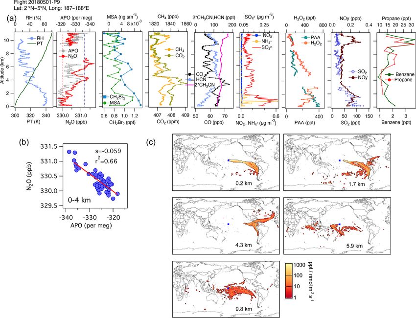
Y. Gonzalez et al.: Impact of stratospheric air and surface emissions                                                       11115

ATom-1 in August 2016). The motivation for this paper is              During sampling, the air passes through a 50-tube Nafion
twofold. Firstly, we present a new retrieval strategy to ac-       drier to remove the bulk water vapor. A Teflon diaphragm
count for the pressure and temperature dependence of laser-        pump downstream of the cell reduces the air pressure
based instruments, and specifically for the use of quantum         to ∼ 60 hPa. Both ambient air and calibration gases pass
cascade laser spectrometers on aircraft. Secondly, we report       through a Teflon dry-ice trap to reduce the dew point to
on the global distribution of N2 O from the surface to 13 km       −70 ◦ C. After ATom-1, we added a bypass between the inlet
and examine the processes contributing to the variability of       and the instrument to increase the flushing rate of the inlet
tropospheric N2 O based on the vertical profiles of N2 O and a     and inlet tubing. The calibration sequence includes 2 min of
broad variety of covariate chemical species and aerosol prop-      ultra-high-purity zero air followed by 1 min each of low- and
erties.                                                            high-mixing ratio gases every 30 min (see Fig. S2). We mea-
                                                                   sured zero air every 15 min during ATom-1 and -2, and every
                                                                   30 min during ATom-3 and -4. A data logger (CR10X, Camp-
2     Instrument specifications, spectral analysis, and            bell Scientific) was used to automate the sampling sequence.
      calibration                                                  The CR10X controlled the pressure controller on the cell and
                                                                   managed the data transfer.
2.1    Specifications of QCLS
                                                                      We use gas cylinders traceable to the National Oceanic and
We measured N2 O mixing ratios with the Har-                       Atmospheric Administration World Meteorological Organi-
vard/NCAR/Aerodyne Research Inc. Quantum Cascade                   zation scales for calibration (NOAA-WMO-X2004A scale
Laser Spectrometer (QCLS). This instrument was previously          for CH4 , WMO-X2014A for CO, and NOAA-2006A for
deployed on the NCAR/NSF Gulfstream V for the HIAPER               N2 O). These gas standards were recalibrated before, during
Pole-to-Pole Observations mission (HIPPO, Wofsy et al.,            and after the deployments to maintain traceability. The low
2011; https://www.eol.ucar.edu/field_projects/hippo, last          mixing ratio gas cylinder contained 298.5 ± 0.3 ppb of N2 O,
access: 14 October 2020) and the O2 / N2 Ratio and CO2             1692.4 ± 0.2 ppb of CH4 , and 119.1 ± 0.3 ppb of CO. The
Southern Ocean Study (ORCAS, Stephens et al., 2018;                high mixing ratio gas cylinder contained 399.1 ± 0.3 ppb of
https://www.eol.ucar.edu/field_projects/orcas, last access:        N2 O, 2182.5 ± 0.3 ppb of CH4 , and 192.8 ± 0.5 ppb of CO.
14 October 2020). Detailed information about the spectrom-         Detailed information on calibrations of the gas cylinders used
eter configuration can be found in Jiménez et al. (2005,           during ATom is given in Table S1 of the Supplement.
2006) and Santoni et al. (2014). A brief description follows.         QCLS also measures carbon dioxide (CO2 ) in a separate
   QCLS provides continuous (1 Hz) measurements of N2 O,           unit. Detailed information about QCLS CO2 measurements
methane (CH4 ), and carbon monoxide (CO) using two ther-           can be found in Santoni et al. (2014).
moelectrically cooled pulsed quantum cascade lasers, a 76 m
pathlength multiple-pass absorption cell (∼ 0.5 L volume),         2.2   Spectral analysis and calibration
and two liquid-nitrogen-cooled solid-state HgCdTe detec-
tors. All these components are mounted on a temperature-           QCLS was damaged during shipping to the deployment site
stabilized, vibrationally isolated optical bench. The temper-      before the start of ATom-1, and the resulting alteration in
ature in QCLS is controlled by Peltier elements coupled            the optical alignment modified the sensitivity of the instru-
with a closed-circuit recirculating fluid kept at 288.0 ± 0.1 K.   ment to temperature and pressure changes during aircraft
QCLS measures CH4 and N2 O by scanning the spectral in-            maneuvers. This increased sensitivity was observed in all
terval of 1275.45 ± 0.15 cm−1 . A second laser is used to scan     ATom deployments. At constant altitude, instrumental pre-
CO at 2169.15 ± 0.15 cm−1 . The supply currents to QCLS            cision was similar to the precision measured during HIPPO
are ramped at a rate of 3.8 kHz to scan the laser frequency        (see the Allan–Werle variance analysis in Fig. 2 in Santoni
for 200 channels (steps in frequency) in laser 1 and 50 chan-      et al., 2014 for HIPPO and Fig. S3 for ATom), but drifts
nels in laser 2; an extra 10 channels are used to measure the      were observed during altitude changes due to the effects of
laser shut off (zero-light level). The spectra and fit residuals   changes in cabin pressure and temperature on the spectral
for CH4 , N2 O, and CO are shown in Fig. S1 of the Supple-         location of interference fringes that arise in the optical path
ment. Mixing ratios are derived at a rate of 1 Hz by a least-      outside the sample cell. In addition, flight altitude changes
squares spectral fit assuming a Voigt line profile at the pres-    mechanically stressed the optical elements surrounding the
sure and temperature measured inside the sample cell and           cell, further modulating fringes or changing the shape of the
using molecular line parameters from the HIgh-resolution           detected laser intensity profile. These spectral artifacts ulti-
TRANsmission molecular absorption database (HITRAN,                mately reduced the accuracy of mixing ratios retrieved from
Rothman et al., 2005). The temperature and pressure inside         spectral fitting. The spectral artifacts most strongly affected
the cell are monitored with a 30 k thermistor and a capaci-       the measurements of CH4 and N2 O. Several post-processing
tance manometer (133 hPa full scale), respectively.                methods using the TDL-Wintel software were explored to
                                                                   improve the precision and accuracy of ATom QCLS N2 O
                                                                   data, most with little success. Since the measured spectra

https://doi.org/10.5194/acp-21-11113-2021                                        Atmos. Chem. Phys., 21, 11113–11132, 2021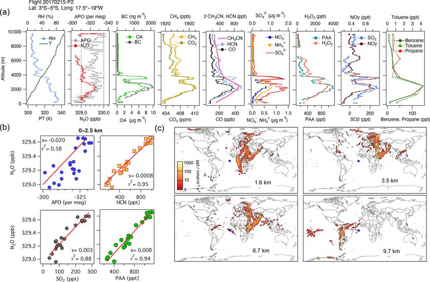
11116                                                  Y. Gonzalez et al.: Impact of stratospheric air and surface emissions

were all saved, it is possible to refit the data with different     1. We paired the mixing ratio records with the correspond-
fit parameters. A limited number of interference fringes may           ing spectra (1 s resolution) for each species (CH4 and
be included in the set of fitting functions. However, none of          N2 O).
the previously used full refitting strategies significantly im-
proved the data accuracy.                                           2. We grouped the mixing ratios and spectra by type –
    We have achieved significant improvements in the preci-            into calibrations (zeros, low span, and high span) and
sion and accuracy of the ATom QCLS N2 O data using a                   air samples – and by time. The spectral data were thus
new method dubbed the “Neptune algorithm,” developed by                arranged in an array with point number in the spectrum
Aerodyne Research, Inc., and that method has been further              as x and spectrum number as y. We calculated an aver-
developed and applied to the data sets described here. Us-             age spectrum for each group type and subtracted these
ing this algorithm, the precision of the retrieved N2 O data           from each individual spectrum within a group.
measured with the damaged QCLS was similar to that re-              3. We zeroed out the spectral arrays at the positions of the
ported in HIPPO. The Neptune algorithm generates correc-               absorption lines to concentrate on the fluctuations ob-
tions to the mixing ratios retrieved from the original fits by         served in the baseline and to prevent the PCA from find-
associating specific spectral features with anomalies in re-           ing line-depth fluctuations as relevant vectors during the
trieved mixing ratios observed during calibrations, i.e., dur-         calibrations. Some degree of smoothing (in x) was ap-
ing intervals when the mixing ratios are held constant. The            plied to the subtracted spectra so that high-frequency
spectral baseline is defined as the spectral channels outside          fluctuations, which have little influence on the mixing
the boundaries of the spectral lines of the target gas. Fluctu-        ratio determination, are not represented. An example of
ations in the spectral baselines are quantified for the entire         such a processed spectral array is shown in Fig. 1a.
data set by means of principal component analysis (PCA).
PCA provides an efficient description of the spectral fluctu-       4. We applied PCA to the whole line-zeroed spectral ar-
ations, naturally producing an ordered set from the strongest          ray to evaluate the fluctuations. PCA was applied in
to the weakest orthogonal vectors (spectral forms), each with          two steps: multiply the spectral array by its transpose
an amplitude history spanning the data set. The PCAs are de-           to generate an autocovariance array and then perform
fined by an optimization procedure during calibrations, when           singular value decomposition on the autocovariance ar-
mixing ratio fluctuations are designed to be ∼ 0. The finite           ray. The PCA generated an efficient description of how
fluctuations in retrieved mixing ratios during calibrations are        the baseline of the spectrum changed with cabin pres-
fitted in the spectral space of the baseline as linear combina-        sure and temperature. The description of spectral fluc-
tions of the leading PCA vector amplitudes, creating a lin-            tuations consisted of a set of products of vectors and
ear combination of amplitudes of spectral fluctuations that            amplitudes.
predict errors in the mixing ratios for each gas for an entire
                                                                    5. We fitted the spectra to the PCAs to express mixing ratio
flight. The error-producing linear combination of amplitudes
                                                                       fluctuations during the set of calibrations and zeros as a
of PCA spectral fluctuations produces a full set of anomaly
                                                                       linear combination of PCA vector histories. The number
estimates that are subtracted from the retrieved mixing ratios
                                                                       of vector histories included in the fit is typically limited
during the flight. The computational time for a 10 h long data
                                                                       to less than 30 because the weaker PCA amplitudes tend
set is only seconds, so variations in the algorithm’s param-
                                                                       to just describe random noise.
eters (i.e., how many PCAs are retained) can be optimized
rapidly.                                                             The linear combination of amplitudes that links spectral
    The Neptune–PCA analysis improved the overall preci-          fluctuations in the baseline to mixing ratio fluctuations dur-
sion by a factor of four for CH4 and a factor of three in         ing calibrations was then applied to the full data set. That
the case of N2 O with respect to the precision of the origi-      generated the retrieval errors for uncalibrated mixing ratios
nal retrievals, as measured by the standard deviation of the      for the whole time series. We subtracted the errors from the
retrieved mixing ratios during calibrations. The repeatability    initial retrievals from the TDLWintel-QCLS software and
of the retrieved calibrations was 0.2 ppb for N2 O and 1 ppb      computed calibrated mixing ratios using the corrected re-
for CH4 (Fig. S4). The laser path of the CH4 / N2 O laser was     trievals for both calibrations and samples. An example of the
realigned between ATom-1 and -2, and the Neptune retrieval        result of applying the Neptune algorithm to the N2 O sam-
was applied to CH4 and N2 O measurements corresponding            ples and calibrations for the ATom-4 flight on 12 May 2018
to the ATom-2, -3, and -4 deployments. Mixing ratios of           is shown in Fig. 1b. The approach used here to minimize the
CH4 and N2 O could not be retrieved during ATom-1 because         effect of changes in pressure and temperature in optical in-
light levels were too low for the CH4 / N2 O laser due to the     struments was based on the observation of fluctuations of the
damage-induced misalignment.                                      baseline during calibrations. Hence, this methodology does
    The steps involved in the Neptune correction process were     not provide any improvement in cases where altitude changes
as follows:                                                       occurred during sampling but not during any of the calibra-
                                                                  tions for an individual flight. Due to frequent calibrations,

Atmos. Chem. Phys., 21, 11113–11132, 2021                                         https://doi.org/10.5194/acp-21-11113-2021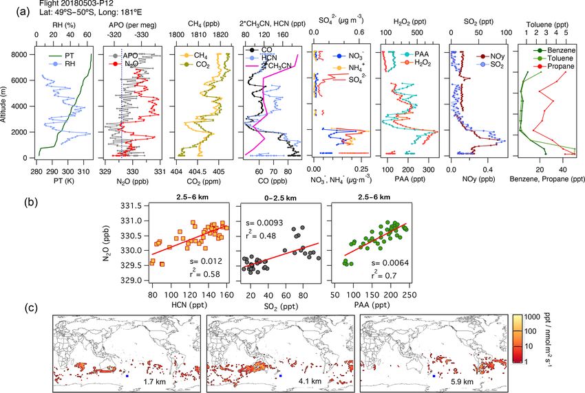
Y. Gonzalez et al.: Impact of stratospheric air and surface emissions                                                             11117

                                                                        the airborne data and the ground-based measurements in the
                                                                        NOAA reference network.

                                                                        3.1   Comparison between airborne N2 O measurements

                                                                        Measurements of N2 O on the DC-8 during ATom were
                                                                        obtained by four instruments: (i) the Unmanned Aircraft
                                                                        Systems Chromatograph for Atmospheric Trace Species
                                                                        (UCATS, Hintsa et al., 2021), (ii) the PAN and other Trace
                                                                        Hydrohalocarbon ExpeRiment (PANTHER; Moore et al.,
                                                                        2006; Wofsy et al., 2011), (iii) the Programmable Flask Pack-
                                                                        age Whole Air Sampler (PFP; Montzka et al., 2019), and
                                                                        (iv) our 1 Hz QCLS.
                                                                           We compared QCLS, PANTHER, and UCATS
                                                                        at 10 s intervals, as provided in the ATom merged
                                                                        file MER10_DC8_ATom-1.nc available at the Oak
                                                                        Ridge      National    Laboratory        Distributed   Active
                                                                        Archive Center (ORNL-DAAC, Wofsy et al., 2018,
                                                                        https://doi.org/10.3334/ORNLDAAC/1581, last access:
                                                                        28 February 2021). The ATom file MER-PFP merged with
                                                                        the PFP sampling interval (also available in the above reposi-
                                                                        tory) was used to compare QCLS and PFP data. A one-to-one
                                                                        comparison between these instruments showed an approxi-
                                                                        mately 1 ppb positive bias in N2 O mixing ratios from QCLS
                                                                        (see Fig. 2a1–a3). The 95 % confidence interval of the mean
                                                                        difference for each pair (95 % C.I.) was 0.75 ± 0.04 ppb
Figure 1. (a) A processed spectral array from the ATom-4 flight on      between QCLS and PANTHER, 1.13 ± 0.03 ppb between
12 May 2018. “Channel” represents a point number in the spectra.        QCLS and UCATS, and 1.18 ± 0.09 ppb between QCLS
Spectra have been grouped by type (i.e., calibration or ambient),       and PFP, respectively, for the full data set (ATom-2, -3,
with averages subtracted, absorption lines zeroed out (near chan-       and -4). Information about the coefficients of the linear
nels 75, 140, and 225). This residual spectral array is then smoothed   fit for each instrument comparison and the 95 % C.I. of
with a binomial filter where the filter width corresponds to the        the difference for each pair are shown in Table S2. The
linewidth of the original spectra. Shifts in fringe phases during al-
                                                                        offset that QCLS N2 O shows against PFP N2 O coincides
titude changes are apparent. (b) Time series of ambient air samples
                                                                        with the offset already reported by Santoni et al. (2014)
and high-span, low-span, and zero calibrations for the same flight
as (a). Green dots are the original N2 O data record. Black dots are    during HIPPO in 2009–2011, which may be attributed to
the N2 O data corrected with Neptune (no calibration applied at this    our calibration procedure. PFP flasks are considered the
point).                                                                 reference measurement on board as the flasks are analyzed
                                                                        with excellent precision and accuracy.

we did not observe this rare scenario in the whole mission.             3.2   Comparison between airborne and surface
To evaluate the ultimate accuracy of our measurements, we                     measurements of N2 O
compared the QCLS N2 O measurements with other onboard
N2 O measurements as well as with the surface N2 O measure-             We evaluated the traceability of lower-troposphere N2 O mix-
ments of stations located along the flight tracks.                      ing ratios by ATom by comparing the four airborne in-
                                                                        struments with the surface measurements of N2 O from the
                                                                        NOAA flask sampling network. If a surface station was en-
3   Accuracy of N2 O measurements from QCLS                             countered within a latitude range of 5◦ north and south with
                                                                        respect to the flight track during a flight, that surface station
We evaluated N2 O mixing ratios measured by QCLS against                was used in the study.
three other instruments that measured N2 O on the NASA                     The mean value of N2 O within that latitude grid of ± 5◦
DC-8 aircraft during ATom. In addition, we compared the set             and at instrument altitudes of 1–4 km was compared with the
of four airborne measurements to data from the flask sam-               mean N2 O observed at the surface station during the period
pling network at ground stations from the NOAA Global                   ± 5 d relative to the flight (due to the non-daily frequency
Monitoring Laboratory (GML, https://gml.noaa.gov/, last ac-             of flask samples). We chose the altitude range between 1 to
cess: 10 December 2020) to evaluate the differences between             4 km to agree with the low free tropospheric conditions that

https://doi.org/10.5194/acp-21-11113-2021                                             Atmos. Chem. Phys., 21, 11113–11132, 2021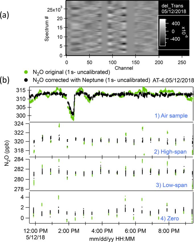
11118                                                     Y. Gonzalez et al.: Impact of stratospheric air and surface emissions

Figure 2. (a) Comparisons between Neptune-corrected QCLS N2 O and (1) UCATS N2 O, (2) PANTHER N2 O, and (3) PFP N2 O for
ATom-2 (orange circles), ATom-3 (green stars), and ATom-4 (blue squares). We used the 10 s averaged merged file to compare QCLS,
UCATS, and PANTHER data. The PFP flask samples had longer sampling times (30 s to a few minutes). The 1 : 1 line is shown as a
dashed line. (b) Comparisons between NOAA N2 O surface flask measurements and Neptune-corrected and airborne data from (1) QCLS
N2 O, (2) UCATS N2 O, (3) PANTHER N2 O, (4) and PFP N2 O for ATom-2, -3, and -4, similar to (a1)–(a3). The solid line shows the 1 : 1
relationship + offset. For plots (b1)–(b4), the airborne data are the mean N2 O values within ± 5◦ of latitude of each surface station and
between 1 and 4 km.

characterized most of the selected ground stations. Informa-           ate the impact of stratospheric air and meridional transport
tion about the surface stations used here is shown in Table S3         of N2 O emissions on N2 O tropospheric column measure-
of the Supplement.                                                     ments over the ocean basins. In the following section, we
   The comparison of the whole data set (ATom-2, -3, -                 define the boundary conditions that were used to evaluate
4) shows that, overall, QCLS and PANTHER overesti-                     that impact, which were based on the NOAA Greenhouse
mated N2 O mixing ratios with respect to the surface data              Gas Marine Boundary Layer Reference from the NOAA
by 1.37 ± 0.35 and 0.44 ± 0.51 ppb (95 % C.I.), respectively.          GML Carbon Cycle Group (NOAA/ESRL GML CCGG,
In contrast, UCATS and PFP showed low bias with re-                    https://gml.noaa.gov/, last access: 10 December 2020). The
spect to the surface data: 0.27 ± 0.37 and 0.008 ± 0.34 ppb            NOAA-MBL N2 O product is a synthetic latitude profile gen-
(95 % C.I.), respectively (Fig. 2b1–b4). Due to the excellent          erated at 0.05 sine latitude and weekly resolution from in-
agreement between PFP and the surface stations and the con-            dividual flask measurements of marine boundary-layer sur-
sistent offset that QCLS showed against PFP and the sta-               face stations distributed along the two ocean basins, and
tions, the QCLS N2 O data presented in the following sec-              provides the scenario needed to evaluate the traceability of
tions of this publication were corrected by subtracting the            aircraft measurements relative to ground measurements at
offset with respect to the PFP data onboard in each deploy-            remote sites (https://gml.noaa.gov/ccgg/arc/?id=13, last ac-
ment: 1.03 ± 0.13 ppb in AT-2, 1.49 ± 0.19 ppb in AT-3, and            cess: 10 December 2020).
1.18 ± 0.17 ppb in AT-4. The final official archive data file
includes a new column where these corrections have been
applied (N2 O_QCLS_ad).                                                4   Results and discussion
   These results show the very close comparability of the
ATom airborne N2 O instruments (differences were < 0.5 ppb             The vertical profiles of N2 O from ATom provide a global
for UCATS and PANTHER instruments and 0 ppb in the                     overview of the N2 O distribution in the troposphere, with ob-
case of PFP) relative to the surface stations and demonstrate          servations performed over the Pacific and Atlantic basins. For
the feasibility of using ATom N2 O measurements to evalu-              this study, we do not include data collected over and close to

Atmos. Chem. Phys., 21, 11113–11132, 2021                                                https://doi.org/10.5194/acp-21-11113-2021
Y. Gonzalez et al.: Impact of stratospheric air and surface emissions 11119
land. In ATom, N2 O ranged between 280 and 335 ppb over 4.1 Impact of stratospheric air on tropospheric N2 O
the oceans. In each season, the lowest N2 O mixing ratios mixing ratios during ATom
are observed at high latitudes (HL, > 60◦ ) in the UT/LS (8–
12.5 km), in air transported downward from the stratosphere. We observe the strongest depletions (> 5 ppb) in N2 O mixing
The highest N2 O mixing ratios are found close to the Equa- ratios at high latitudes and altitudes, consistent with strato-
tor (30◦ S–30◦ N, 326 to 335 ppb), and extend along the tro- spherically influenced air (Fig. 3). Stratosphere–troposphere
pospheric column up to 6 km. They are influenced by con- exchange processes allow stratospheric-depleted N2 O to be
vective activity over the tropical regions (Kort et al., 2011; distributed throughout the troposphere. The NOAA surface
Santoni et al., 2014). At mid-latitudes (ML, 30–60◦ N), tro- network shows a seasonal minimum of N2 O 2–4 months later
pospheric N2 O values range between 322 and 333 ppb. Tro- than the stratospheric polar vortex break-up season. This sea-
pospheric N2 O tends to increase towards northern latitudes sonal minimum is observed at the surface around May in the
as a result of higher anthropogenic emissions in the North- Southern Hemisphere and around July in the Northern Hemi-
ern Hemisphere relative to the Southern Hemisphere. More sphere (see Figs. S8 and S9) (see Nevison et al., 2011 and ref-
details on the variability of N2 O mixing ratios along the tro- erences therein). The enhanced downwelling of the Brewer–
pospheric column are described in Sect. S1. Dobson circulation (BDC) in late winter–spring reinforces
We study the impact of N2 O sources and stratospheric air the downward transport of stratospheric air depleted in N2 O
on the N2 O column based on the anomalies (enhancements throughout the free troposphere (1–8 km), as observed in Oc-
and depletions) we observed in the airborne N2 O mixing ra- tober in the Southern Hemisphere (ATom-3, Fig. 3c and f)
tios relative to the N2 O “background,” defined here as the and in May in the North Atlantic (ATom-4, Fig. 3e). The N2 O
NOAA-MBL product. We use the NOAA-MBL product to depletion is likely the result of stratospheric air being moved
constrain a latitudinal gradient of N2 O mixing ratios at the downwards by the BDC and trapped by the polar vortex, with
surface for each deployment. These data have been widely a more pronounced effect in the Southern Hemisphere, where
used to estimate the N2 O background (Assonov et al., 2013; the polar vortex is stronger. These results support previous
Nevison et al., 2011). More information about the NOAA- work suggesting that downward transport of stratospheric air
MBL product and the latitudinal gradient of their measure- with low N2 O exerts a strong influence on the variance of tro-
ments is discussed in Sect. S2. This approach highlights the pospheric N2 O mixing ratios (Nevison et al., 2011; Assonov
extra information that aircraft profiles can provide. Cross- et al., 2013).
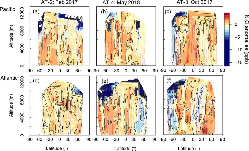
sections of N2 O anomalies are shown in Fig. 3. The data The impact of stratosphere-to-troposphere transport can
describe the overall homogeneity of N2 O in the troposphere be studied by combining information on tracers of strato-
(30 % of the anomalies ranged between ± 0.5 ppb). We sup- spheric air such as ozone (O3 from the NOAA – NOy O3 ;
pose that the ± 0.5 ppb interval accounts for the day-to-day Bourgeois et al., 2020), sulfur hexafluoride (SF6 from PAN-
and seasonal variability of N2 O. Episodes of N2 O depletion THER), CFC12 (from PANTHER), and carbon monoxide
(< −0.5 ppb) that relate to the influence of stratospheric air (CO from QCLS). These tracers are usually used either be-
are observed in 53.5 % of the aircraft samples during ATom-2 cause they are strongly produced in the stratosphere (e.g.,
to -4, whereas episodes of N2 O enhancement (> 0.5 ppb) that O3 ) or because they are tracers of anthropogenic emissions
relate to the contribution of N2 O sources account for 16.5 % in the troposphere with a strong stratospheric sink (e.g.,
of the calculated anomalies. CO, SF6 , and CFC12 ). In addition, meteorological parame-
Trajectories and associated surface influence functions ters such as potential vorticity (PV), the product of absolute
were computed using the Traj3D model (Bowman, 1993) vorticity and thermodynamic stability (PV was generated by
and wind fields from the National Center for Environmen- GEOS5-FP for ATom), can be used to trace the stratosphere-
tal Prediction Global Forecast System (NCEP GFS). Model to-troposphere transport.
trajectories were initialized at receptors spaced 1 min apart Overall, the interhemispheric gradient of N2 O is much
along the ATom flight tracks, followed backwards for 30 d, smaller than those of CO and SF6 (Fig. 4), but the differ-
and reported at 3 h resolution. From these trajectories, we ence for each species is driven by larger anthropogenic emis-
calculated the surface influence for each receptor point (foot- sions in the Northern Hemisphere. The tracer–tracer corre-
prints in units of concentration mixing ratio per emission lations shown in Fig. 4 show different patterns. The linear
flux; ppt nmol−1 m2 s). The footprint can be convolved with trend between N2 O and O3 or CFC-12 highlights the role
a known flux inventory of a nonreactive gas to calculate the of depletion (N2 O and CFC-12) and production (O3 ) in the
expected enhancement/depletion of that gas for each receptor stratosphere (Fig. 4a1, a4). When N2 O is plotted against the
point. anthropogenic tracers CO and SF6 , two distinct trends are
observed. Tropospheric N2 O can be identified as the hori-
zontal band containing high N2 O (> 328 ppb) and variable
CO and SF6 , whereas the vertical band with variable N2 O
and small changes in CO and SF6 is due to the mixing be-
tween tropospheric air and stratospheric air depleted in N2 O
https://doi.org/10.5194/acp-21-11113-2021 Atmos. Chem. Phys., 21, 11113–11132, 2021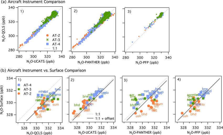
11120                                                      Y. Gonzalez et al.: Impact of stratospheric air and surface emissions

Figure 3. Cross-sections of N2 O anomalies (ppb) representing the differences between the airborne N2 O (10 s resolution) and the surface
N2 O mixing ratios, interpolated to 0.25◦ latitude and 250 m altitude for each deployment. Shown are the N2 O anomalies over (a)–(c) the
Pacific and (d)–(f) the Atlantic, with each column representing a deployment (ordered by season: ATom-2, -4, and -3). The color scale
ranges from −15 to 5 ppb. Values between −50 and −15 ppb, observed at the highest altitudes (> 10 km), are shown in white to allow
better visualization of small changes in positive anomalies. Lilac dashed lines represent the flight tracks. Black contours are areas of N2 O
anomalies.

(Fig. 4a1–a3). The N2 O versus CO plot shows an L-shaped                 stratosphere-to-troposphere transport events at mid-latitudes
(bimodal) curve similar to those typically observed in O3 –              in the region between May and July (Fig. 3e; Cuevas et al.,
CO correlations during stratosphere-to-troposphere airmass               2013 and references therein). Anomalies in PV relative to
mixing events (Fig. 4a2, Krause et al., 2018). A quasi-vertical          its mean latitudinal distribution in the free troposphere (2–
line in the N2 O–CO plot (i.e., constant CO) is indicative               8 km) highlight events involving the strong downward trans-
of a strong impact of stratospheric air, as the stratospheric            port of stratospheric air. Negative PV, N2 O, CO, and CFC-12
equilibrium mixing ratio of CO is observed (Krause et al.,               anomalies (positive for O3 ) describe the transport of strato-
2018). The lower the CO background, the greater the in-                  spheric air into the troposphere in the SH, whereas positive
fluence of the stratospheric air during the airmass mixing               PV and negative N2 O, CO, and SF6 anomalies (positive for
(North Atlantic high latitudes in Fig. 4a2) and vice versa.              O3 ) describe the downward transport of stratospheric air in
A strong correlation is also indicative of rapid mixing be-              the NH (Fig. 4b1–b4). The correlations between N2 O and PV
tween the two air masses. During ATom, the strongest im-                 and the similarities with CFC-12 indicate that stratosphere-
pact of stratospheric air was observed in the Pacific mid- and           to-troposphere exchange leads to variations in tropospheric
high latitudes in February (ATom-2) and in the Atlantic in               N2 O of up to 10 ppb at the higher latitudes for the alti-
May (ATom-4, Fig. S11). At the North Pacific mid- and high               tudes covered during the flights. This influence is notably
latitudes (NMHL > 30◦ N), we find a consistent linear re-                larger than the 2–4 ppb enhancements associated with re-
lationship between N2 O and O3 , with a relatively constant              gional emissions (see below).
N2 O / O3 slope (−0.05 to −0.04) during all seasons. Linear
correlations between N2 O and CFC-12 highlight the domi-                 4.2   Impact of emissions on tropospheric N2 O mixing
nant influence of stratospheric air that was depleted in these                 ratios during ATom
two substances in the range of mixing ratios observed at mid-
and high latitudes (Fig. S11).                                           During ATom, episodes of positive N2 O anomalies relative
   During spring, the mid-latitudes are strongly impacted by             to the surface station MBL reference occurred close to the
stratospheric air due to the occurrence of tropopause folds              equator (Fig. 3a–c) and in a few locations at mid-latitudes
and cutoff lows to the south of the westerly subtropical jets            in both ocean basins across all seasons. We used the infor-
(Hu et al., 2010 and references therein). The stronger deple-            mation from the vertical profiles, including back trajecto-
tion of N2 O mixing ratios observed over the Atlantic relative           ries and correlated chemical tracers, to trace the origins of
to the Pacific during spring is due to a greater number of deep          these enhancements. We investigated data on CO, CH4 , and

Atmos. Chem. Phys., 21, 11113–11132, 2021                                                 https://doi.org/10.5194/acp-21-11113-2021
Y. Gonzalez et al.: Impact of stratospheric air and surface emissions 11121
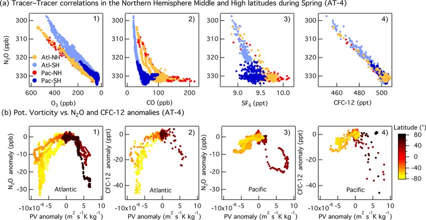
Figure 4. (a) Correlations between N2 O and O3 (a1), CO (a2), SF6 (a3), and CFC-12 (a4) at mid- and high latitudes (30–85◦ N) during
Northern Hemisphere spring (ATom-4). The data are colored as a function of the ocean basin and hemisphere: North Pacific mid–high
latitudes (Pac-NH, > 30◦ N) in red, South Pacific mid–high latitudes (Pac-SH, < 30◦ S) in dark blue, South Atlantic mid–high latitudes (Atl-
SH, < 30◦ S) in light blue, and North Atlantic mid–high latitudes (Atl-NH, > 30◦ N) in orange. Note that the N2 O and O3 axes are reversed.
(b) Correlations between anomalies in potential vorticity relative to its mean latitudinal distribution in the free troposphere (2–8 km) and
anomalies in N2 O (b1, b3) and CFC-12 (b2, b4) as a function of latitude during spring (ATom-4) over the Pacific and Atlantic basins.
Mid-latitudes are shown in orange in the SH and in light brown in the NH.
CO2 measured by QCLS and NOAA Picarro 2401 m; hydro- correlated with SO2 and enhanced PM1 particles, and ver-
gen cyanide (HCN), sulfur dioxide (SO2 ), hydrogen perox- tical gradients were sometimes correlated with gradients of
ide (H2 O2 ), and peroxyacetic acid (PAA) measured with the APO and HCN.
California Institute of Technology Chemical Ionization Mass Several N2 O peaks are observed together with enhance-
Spectrometer (CIT-CIMS, Crounse et al., 2006; St. Clair et ments of H2 O2 and PAA, which are primarily formed in
2−
al., 2010); ammonium (NH+ −
4 ), sulfate (SO4 ), nitrate (NO3 ), chemical processes that occur in the atmosphere. For the al-
and organic aerosols (OA) from the Colorado University Air- titude range 2–4 km, regressions produced r 2 > 0.7 for 16
craft High-Resolution Time-of-Flight Aerosol Mass Spec- profiles of N2 O vs. H2 O2 and 15 profiles of N2 O vs. HCN
trometer (HR-AMS, DeCarlo et al., 2006; Canagaratna et al., (a tracer for combustion of biomass), but only three such
2007; Jimenez et al., 2019; Guo et al., 2021; Hodzic et al., profiles produced these strong associations for both H2 O2
2020); NOy from the NOAA NOy O3 four-channel chemilu- and HCN in common. Some of these profiles also showed
minescence instrument (CL, Ryerson et al., 2019); CH2 Br2 , correlated enhancements of SO2 and NO (nine profiles with
CH3 CN, benzene, and propane from the NCAR Trace Or- r 2 > 0.6). This result raises the question of whether globally
ganic Gas Analyzer (TOGA, Apel et al., 2019); and atmo- significant production of N2 O may be occurring in hetero-
spheric potential oxygen (APO ≈ O2 + 1.1 × CO2 ) from the geneous reactions involving SO2 , NO redox chemistry, and
NCAR Airborne Oxygen Instrument (AO2, Stephens et al., HONO near to strong sources of reactive pollutants, which
2020). have been observed in heavily polluted atmospheres (Wang
We calculated the correlations between N2 O and the men- et al., 2020) and have been theorized to occur in the plumes
tioned species in three layers (0–2000, 2000–4000, and of refineries or power plants (e.g., Pires and Rossi, 1997).
4000–6000 m). Correlation coefficients in each layer for a In most cases, because we were sampling in the middle of
given profile were calculated using a minimum threshold each ocean and not over the source regions, it was not pos-
of 15 data points per layer. These profiles show that many sible to distinguish between the different sources that con-
of the most prominent enhancements of N2 O are closely as- tributed to the observed N2 O enhancements. We also ob-
sociated with pollutants such as HCN, CH3 CN, H2 O2, , and served that the impacts of the different sources on N2 O mix-
other pollutants associated with combustion and photochem- ing ratios were region dependent. Here, we describe, with
ical air pollution. Some profiles show peaks that are closely some examples, the sources that contribute to the major N2 O
https://doi.org/10.5194/acp-21-11113-2021 Atmos. Chem. Phys., 21, 11113–11132, 202111122 Y. Gonzalez et al.: Impact of stratospheric air and surface emissions
enhancements observed during ATom by oceanic region, al- (r 2 > 0.7) between N2 O and APO (or δ(O2 / N2 ), which has
though we cannot precisely pinpoint the source processes. lower measurement noise) for altitude bins 0–2 (8) and 2–
4 km (1), with back trajectories indicating that they origi-
4.2.1 N2 O enhancements over the Pacific nated close to the west coast of North America and the Mau-
ritanian coast as well as in the equatorial Pacific. The median
Episodes of N2 O enhancement were frequently observed at slope of regressions of APO vs. N2 O for these profiles in
mid-latitudes in the southern Pacific Ocean, and these were ATom is −0.04 ppb per meg, and the mean is −0.05 (± 0.04,
linked by the associated footprints to emissions over the con- 1σ ) ppb per meg – very similar to the range found by Gane-
tinents. In this region, N2 O enhancements are predominantly san et al. (2020) and Lueker et al. (2003) in coastal areas.
associated with air masses with enhanced H2 O2 , PAA, and An example is shown in Fig. 6 for 1 May 2018. We ob-
CO. For example, consider Fig. 5, which shows data from serve a high correlation between N2 O and APO (r 2 = 0.66)
profile 12, obtained at 49.5–50◦ S and near the Date Line on between 0 and 4 km altitude. At these altitudes we also see
3 May 2018. A distinct peak in N2 O of amplitude 1 ppb at enhancements in dibromomethane (CH2 Br2 ), a tracer of phy-
1700 m altitude is significantly correlated with enhancements toplankton biomass (Liu et al., 2013 and references therein),
in CH3 CN. These associations and the footprints suggest a consistent with a marine biological flux of halogenated
regional contribution from fuel types from the industrial zone VOCs (Asher et al., 2019), dimethyl sulfide (DMS), and
of Australia (Fig. 5c), which is also supported by the aerosol methanesulfonic acid (MSA), the main particulate product of
characterization from PALMS (not shown for brevity). In DMS oxidation in the MBL. However, on this flight, the foot-
this profile, close to the surface, the lowest QCLS N2 O mix- prints and the influence of the surface ocean (Fig. S12b) in-
ing ratios agree with the NOAA MBL N2 O (dashed line in dicate that this N2 O gradient represents a difference between
Fig. 5b). At higher altitudes (2.5–6 km), strong correlations sampling a near-surface marine air mass from the south and
between N2 O, H2 O2 , PAA, CO, and HCN but not SO2 sug- a more continental air mass from the east at 4 km (Fig. 6a–
gest the influence of biomass burning from central Australia c). Close to the surface, the lowest QCLS N2 O mixing ra-
(3–5 km) and South America (6 km) (Fig. 5b, middle and tios agree with the NOAA MBL N2 O at the origin of the air
right-hand panels in Fig. 5c, and Fig. S11f). The relatively masses suggested by the footprints (25◦ S, dashed red line
low mixing ratios of short-lived trace gases (PAA, H2 O2 , in Fig. 6b), whereas the lowest QCLS N2 O mixing ratios at
and PM1 aerosols with lifetimes ranging from hours to a few 4 km agree with the NOAA MBL N2 O (dotted blue line in
days) and the surface influence based on the back trajectories Fig. 6b). Thus, the N2 O to APO correlation most likely rep-
(Fig. S13a) indicate that most of these profiles sampled sig- resents the latitudinal and ocean–land gradients established
nificantly aged air masses that were transported for extended for a combination of reasons, with higher APO and lower
periods over the South Pacific. N2 O originating from higher southern latitudes away from
In the equatorial Pacific, episodes of N2 O enhancement continents. During this flight, there were particularly notice-
were frequently associated with a mixture of potential ma- able N2 O variations between 4 and 6 km height that appear to
rine, industrial, and biomass burning emissions. Atmospheric be related to biomass-burning plumes from fires occurring in
potential oxygen (APO) is primarily a tracer of oxygen ex- Venezuela and the Caribbean, in agreement with simultane-
change with the oceans, defined as deviations in the oxygen- ous enhancements in CO and HCN mixing ratios (Fig. 6a, c
to-nitrogen ratio (δ(O2 / N2 )) corrected for changes in O2 and Fig. S12), and there was increasing SO2 in the first 2 km,
due to terrestrial photosynthesis and respiration and for in- which was linked to oil and gas pollution sources near coast-
fluences from combustion (Stephens et al., 1998), lines. The nature of these emissions was also confirmed by
δAPO = δ(O2 /N2 ) + 1.1/XO2 (XCO2 − 350). (1) aerosol characterization using the PALMS instrument (figure
not shown).
Here, δ(O2 / N2 ) is the deviation in the O2 / N2 ratio (per
meg), 1.1 is an approximation to the O2 / CO2 ratio for pho- 4.2.2 N2 O enhancements over the Atlantic
tosynthesis and respiration, XO2 is the mole fraction of O2
in dry air, and XCO2 is the mole fraction of CO2 in the air Much more of a continental influence was observed dur-
sample (dry, µmol mol−1 ). Since APO primarily tracks oxy- ing the Atlantic Basin ATom flights than during the Pacific
gen exchange between the ocean and the atmosphere, APO flights. In the North Atlantic at around 30◦ N during winter,
depletions can indicate marine N2 O emissions from areas we observe small enhancements of N2 O that contrast with
with strong upwelling (Lueker et al., 2003; Ganesan et al., the overall influence of stratospheric air on the tropospheric
2020). However, APO is also sensitive to pollution such as column (AT-2, Fig. 3d). The contribution is much higher dur-
biomass burning and fossil fuel combustion (Lueker et al., ing the fall season (AT-3, Fig. 3f). Several episodes of N2 O
2001) and, because both N2 O and APO have meridional gra- enhancement are associated with enhancements of CH4 , CO,
dients resulting from many influences, correlations can re- and HCN. We also observe some episodes where N2 O in-
sult simply from sampling air transported from different lati- creases while CO2 decreases (figure not shown), which could
tudes. In ATom, nine profiles showed significant correlations reflect the accumulation of agricultural emissions over the
Atmos. Chem. Phys., 21, 11113–11132, 2021 https://doi.org/10.5194/acp-21-11113-2021Y. Gonzalez et al.: Impact of stratospheric air and surface emissions 11123
Figure 5. (a) Vertical profiles of potential temperature (PT), relative humidity (RH), N2 O, APO, CH4 , CO2 , CO, HCN, CH3 CN, NO− +
3 , NH4 ,
SO2+
4 , H2 O2 , PAA (CH3 C(O)OOH), SO2 , NOy , benzene, toluene, and propane from profile 12, obtained on 3 May 2018. The dotted blue
line in the plot of APO and N2 O represents the NOAA-MBL reference (N2 O-MBL) at the latitude of the flight. (b) Correlations between
N2 O and HCN and PAA for altitudes between 2.5 and 6 km, and between N2 O and SO2 for altitudes between 0 and 2.5 km, indicate an
admixture of marine, biomass-burning, urban, and oil and gas industry contributions to N2 O mixing ratios (s represents the slope of the
linear fit). (c) Footprint maps tracing surface regions that influence mixing ratios measured at the altitude ranges of 1–2, 2.5–5, and 5–7 km,
respectively. Blue squares show sampling locations. Values below 3 ppt nmol−1 m2 s are not included. Note that the APO axes are reversed.
summer or just greater sampling of Northern Hemisphere below 4 km. At high altitudes, N2 O enhancements are caused
summer air masses, whereas increases of N2 O with CO are by the interception of polluted air masses from South Amer-
indicators of urban pollution and are, together with HCN, as- ica and the west coast of Africa mixed with the oceanic con-
sociated with a few episodes of biomass burning. tribution to N2 O (∼ 10 km). The N2 O:APO correlations for
The influences of different regions on the N2 O mixing ra- the feature between 1.5 and 3 km most likely represent APO
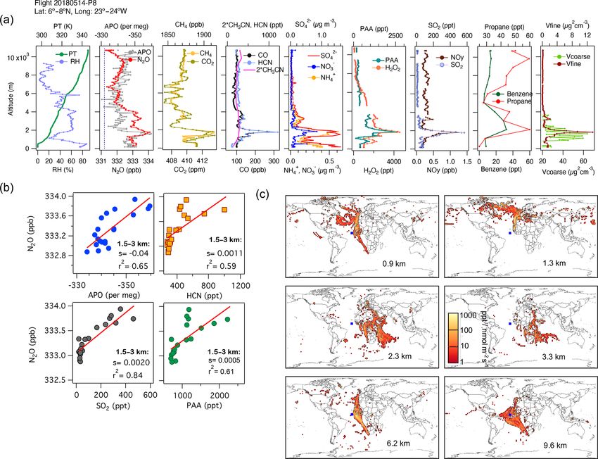
tios over the Atlantic on 14 May 2018 are shown in Fig. 7. depletion through industrial combustion, which is stoichio-
This profile shows the contributions to tropospheric N2 O metrically consistent with the observed increases in CO2 and
from pollution transported down over the Mauritanian coast CH4 for this feature.
from Western Europe, biomass-burning emissions, urban and During ATom, we observed large contributions to the tro-
industrial emissions from southern Africa and the Middle pospheric N2 O over the Atlantic Ocean from Africa, along
East (between 1.5 and 3 km), and polluted air masses from with some contributions from Europe and South America.
South America and the west coast of Africa, which are mixed During AT-2, we found strong correlations in the subtrop-
with the oceanic contribution to N2 O (∼ 10 km, Fig. 7a–c ical and tropical regions over the Atlantic between N2 O,
2−
and Fig. S13). The aerosol characterization (from PALMS, H2 O2 , PAA, HCN, CO, CO2 , SO2 , OA, NH+ 4 , and SO4 at
not shown) indicates that mineral dust and biomass-burning altitudes between 0 and 2.5 km, representing the combined
emissions influence the atmospheric layer between 1 and 2
influence of photochemistry (rN2OvsPAA = 0.94), biomass-
6 km in altitude, while oil combustion influences the layer 2
burning events from the Congo region (rN2OvsHCN = 0.95),
https://doi.org/10.5194/acp-21-11113-2021 Atmos. Chem. Phys., 21, 11113–11132, 202111124 Y. Gonzalez et al.: Impact of stratospheric air and surface emissions
2−
Figure 6. (a) Vertical profiles of PT, RH, and the tracers N2 O, APO, MSA, CH2 Br2 , CH4 , CO2 , CO, HCN, CH3 CN, NO− +
3 , NH4 , SO4 ,
H2 O2 , PAA (CH3 C(O)OOH), SO2 , NOy , benzene, toluene, and propane from profile 9 on 1 May 2018. The dotted blue line in the plot
of APO and N2 O represents the NOAA-MBL reference (N2 O-MBL) at the latitude of the flight; the dashed red line shows the N2 O-MBL
at the origin of the air masses suggested by the footprints (25◦ S). (b) N2 O–APO correlations between 0 and 4 km that possibly describe
the latitudinal gradient of N2 O (s represents the slope of the linear fit). (c) Footprint maps tracing surface regions that influence mixing
ratios measured in the altitude ranges 0–2, 2–4, 3–5, 5–7, and 9–11 km, respectively. Blue squares show sampling locations. Values below
3 ppt nmol−1 m2 s are not included. Note that the APO axes are reversed to illustrate the negative correlation with N2 O.
and the industrial production of N2 O from oil and gas emis- all enhancement. This allowed us to quantify the dominant
2
sions from the Niger River Delta in Africa (rN2OvsSO2 = sources for various layers within each profile. Each of the
0.84). An example is shown in Fig. 8 for 15 February 2017 calculated enhancements was then compared to the enhance-
(see also Fig. S12 and the land contribution in Fig. S13). ment in N2 O observed for the profiles. The observed N2 O
To understand the origin of the enhancements in N2 O, enhancements were calculated relative to the NOAA MBL
we calculated the enhancement expected in the atmosphere reference (Fig. 8a, dashed red line) for each 10 s observa-
based on monthly mean estimates of anthropogenic emis- tion, with background concentrations selected from locations
sions from the Emissions Database for Global Atmospheric close to the origin of the air mass as indicated by the surface
Research (EDGAR, http://edgar.jrc.ec.europa.eu/, last ac- influence (shown as dashed and dotted lines in the N2 O alti-
cess: 5 February 2021). We convolved the calculated surface tude profiles in Figs. 5–8). We also included 0.4 ppb of un-
influence (footprint) with the inventory to calculate the N2 O certainty for the observed enhancements based on our mea-
enhancement expected for each receptor. We also calculated surement precision.
the contribution of each region and source sector to the over-
Atmos. Chem. Phys., 21, 11113–11132, 2021 https://doi.org/10.5194/acp-21-11113-2021Y. Gonzalez et al.: Impact of stratospheric air and surface emissions 11125
2−
Figure 7. (a) Vertical profiles of PT, RH, the tracers N2 O, APO, CH4 , CO2 , CO, HCN, CH3 CN, NO− +
3 , NH4 , SO4 , H2 O2 , PAA, SO2 ,
NOy , benzene, and propane, and the volumes of coarse and fine particles from profile 8 on 14 May 2018. The dotted blue line in the plot of
APO and N2 O represents the NOAA-MBL reference (N2 O-MBL) at the latitude of the flight. (b) Correlations between N2 O and APO, HCN,
SO2 , and propane at altitudes of 1–3 km show possible contributions from marine upwelling, biomass burning, and the oil and gas industry,
as supported by the footprints (s represents the slope of the linear fit). (c) Footprint maps tracing surface regions that influence mixing ratios
measured in the altitude ranges 0–1, 2–4, 4–5, 5–7, and 7–10 km, respectively. The blue square shows the sampling location. Values below
3 ppt nmol−1 m2 s are not included. Note that the APO axes are reversed.
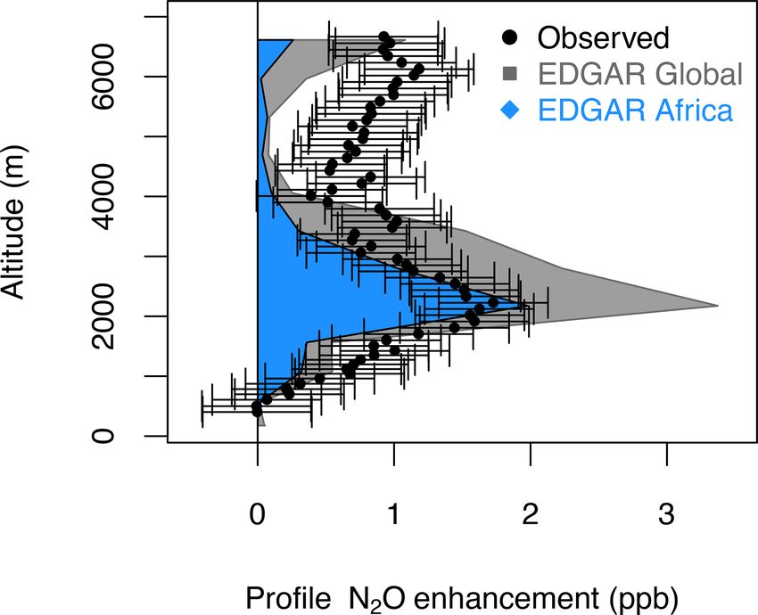
The largest N2 O enhancement (peaking at 2 ppb at 2 km) correlations between N2 O and HCN (r 2 = 0.95), CO, and
observed over the Atlantic during ATom-2 (February 2017; CH3 CN suggest that N2 O from burning emissions also con-
Fig. 9) can be attributed to African agriculture, along with tributes to the N2 O enhancement (Figs. 8 and S12). How-
smaller but significant influences from Asia and Europe ever, when we convolved the monthly mean fire contri-
(0.5 ppb each at 2–4 km, Fig. S14). The observed and mod- butions from the Global Fire Emissions Database (GFED,
eled N2 O enhancements agree within an order of magnitude https://www.globalfiredata.org, last access: 5 February 2021)
for the profile, but the model underestimates the high-altitude with the surface influence footprints (as described above), we
(4–7 km) N2 O enhancement by < 1 ppb and overestimates found that the wildfire-produced N2 O is minimal for this pro-
the lower-altitude enhancement (2–4 km) by ∼ 1 ppb. This file (∼ 0.2 ppb), suggesting that fires of anthropogenic or ur-
difference in N2 O enhancement could be due to a strong ban origin might be the source of that contribution (Figs. 8a–
latitudinal gradient in N2 O across this profile or the timing c, 9, S12, and S13).
of N2 O emissions sampled along this single profile com-
pared to a monthly mean estimate from the inventory. Strong
https://doi.org/10.5194/acp-21-11113-2021 Atmos. Chem. Phys., 21, 11113–11132, 2021You can also read