Time-resolved emission reductions for atmospheric chemistry modelling in Europe during the COVID-19 lockdowns - Recent
←
→
Page content transcription
If your browser does not render page correctly, please read the page content below
Atmos. Chem. Phys., 21, 773–797, 2021
https://doi.org/10.5194/acp-21-773-2021
© Author(s) 2021. This work is distributed under
the Creative Commons Attribution 4.0 License.

Time-resolved emission reductions for atmospheric chemistry
modelling in Europe during the COVID-19 lockdowns
Marc Guevara1 , Oriol Jorba1 , Albert Soret1 , Hervé Petetin1 , Dene Bowdalo1 , Kim Serradell1 , Carles Tena1 ,
Hugo Denier van der Gon2 , Jeroen Kuenen2 , Vincent-Henri Peuch3 , and Carlos Pérez García-Pando1,4
1 BarcelonaSupercomputing Center, Barcelona, 08034, Spain
2 Department of Climate, Air and Sustainability, TNO, Utrecht, the Netherlands
3 European Centre for Medium-Range Weather Forecasts, Reading, UK
4 ICREA, Catalan Institution for Research and Advanced Studies, Barcelona, 08010, Spain

Correspondence: Marc Guevara (marc.guevara@bsc.es)

Received: 8 July 2020 – Discussion started: 22 July 2020
Revised: 7 November 2020 – Accepted: 1 December 2020 – Published: 20 January 2021

Abstract. We quantify the reductions in primary emissions        tion is attributable to road transport, except SOx . The re-
due to the COVID-19 lockdowns in Europe. Our estimates           ductions reached −50 % (NOx ), −14 % (NMVOCs), −12 %
are provided in the form of a dataset of reduction factors       (SOx ) and −15 % (PM2.5 ) in countries where the lockdown
varying per country and day that will allow the modelling        restrictions were more severe such as Italy, France or Spain.
and identification of the associated impacts upon air quality.   To show the potential for air quality modelling, we simulated
The country- and daily-resolved reduction factors are pro-       and evaluated NO2 concentration decreases in rural and ur-
vided for each of the following source categories: energy        ban background regions across Europe (Italy, Spain, France,
industry (power plants), manufacturing industry, road traf-      Germany, United-Kingdom and Sweden). We found the lock-
fic and aviation (landing and take-off cycle). We computed       down measures to be responsible for NO2 reductions of up to
the reduction factors based on open-access and near-real-        −58 % at urban background locations (Madrid, Spain) and
time measured activity data from a wide range of informa-        −44 % at rural background areas (France), with an average
tion sources. We also trained a machine learning model with      contribution of the traffic sector to total reductions of 86 %
meteorological data to derive weather-normalized electricity     and 93 %, respectively. A clear improvement of the modelled
consumption reductions. The time period covered is from          results was found when considering the emission reduction
21 February, when the first European localized lockdown          factors, especially in Madrid, Paris and London where the
was implemented in the region of Lombardy (Italy), until         bias is reduced by more than 90 %. Future updates will in-
26 April 2020. This period includes 5 weeks (23 March until      clude the extension of the COVID-19 lockdown period cov-
26 April) with the most severe and relatively unchanged re-      ered, the addition of other pollutant sectors potentially af-
strictions upon mobility and socio-economic activities across    fected by the restrictions (commercial and residential com-
Europe. The computed reduction factors were combined with        bustion and shipping) and the evaluation of other air quality
the Copernicus Atmosphere Monitoring Service’s European          pollutants such as O3 and PM2.5 . All the emission reduction
emission inventory using adjusted temporal emission pro-         factors are provided in the Supplement.
files in order to derive time-resolved emission reductions per
country and pollutant sector. During the most severe lock-
down period, we estimate the average emission reductions
to be −33 % for NOx , −8 % for non-methane volatile or-          1   Introduction
ganic compounds (NMVOCs), −7 % for SOx and −7 % for
PM2.5 at the EU-30 level (EU-28 plus Norway and Switzer-         Since the end of February 2020, most European coun-
land). For all pollutants more than 85 % of the total reduc-     tries have imposed lockdowns to combat the spread of the
                                                                 COVID-19 pandemic, forcing many industries, businesses

Published by Copernicus Publications on behalf of the European Geosciences Union.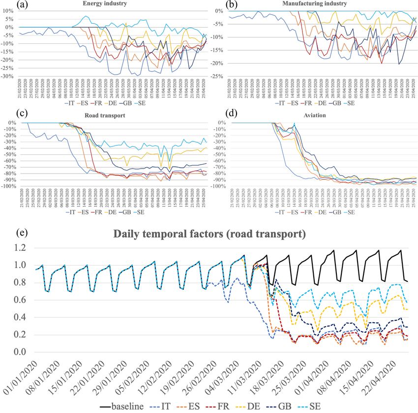
774               M. Guevara et al.: Time-resolved emission reductions for atmospheric chemistry modelling in Europe

and transport networks to either close down or drastically re-     some sectors. Some studies focussing on the quantification of
duce their activity. Such a socioeconomic disruption, which        emission reductions are beginning to be published. Le Quéré
is unprecedented in many ways, has resulted in a sudden drop       et al. (2020) quantified the reduction in daily CO2 emis-
of atmospheric anthropogenic emissions, including both cri-        sions during the COVID-19 lockdown from January 2020
teria pollutants and greenhouse gases. The fall of pollutant       to April 2020 over 69 countries, 50 US states and 30 Chi-
levels across countries has been identified in multiple studies    nese provinces for a total of six sectors of the economy (i.e.
through the analysis of ground-based and satellite air quality     energy industry, manufacturing industry, road transport, res-
observations (e.g. Bauwens et al., 2020; Collivignarelli et al.,   idential sector, public sector and aviation). The study, which
2020; Petetin et al., 2020). While these studies have assessed     calculates the emission reductions based on national activity
changes in pollutant concentrations, further understanding of      data, was focussed on estimating the expected impact of the
the lockdown impacts upon air quality and climate requires         lockdowns upon the 2020 annual CO2 emissions and climate,
quantifying the reduction of primary emissions. Emissions          but it did not include an analysis of emission cuts of criteria
and weather changes are entangled and looking at concentra-        pollutants (NOx , SOx , NMVOCs, NH3 , PM10 and PM2.5 ) or
tion changes only can be largely affected by specific weather      air pollution levels. More recently, Menut et al. (2020) de-
conditions, especially considering that the past winter and        veloped an emission scenario for western Europe to quantify
spring 2020 were exceptionally hot in Europe (C3S, 2017).          the impact of the lockdowns on air quality levels. Although
   Understanding and quantifying the impact of the COVID-          focussing on criteria pollutants, the emission scenario was
19 lockdowns upon European emissions and air quality is            limited to March 2020 and was set up using only the Ap-
difficult due to the heterogeneous implementation of restric-      ple movement trends, which were used to derived emission
tions across different countries, including (i) different start-   reductions not only for road transport but also for other an-
ing dates of the restrictions, (ii) diversity in the levels and    thropogenic sources (i.e. manufacturing industry, non-road
type of restrictions, (iii) changes in time of the restriction     transport and residential–commercial combustion).
levels, and (iv) different spontaneous response by individ-           We present an open-source dataset of day-, sector- and
uals (e.g. voluntary decision to change the way of com-            country-dependent emission reduction factors for Europe as-
muting). The chronology of the lockdowns is illustrated in         sociated with the COVID-19 lockdowns. These factors are
Fig. 1, which shows stringency index trends computed by            designed to support both the quantification of European pri-
the Oxford COVID-19 Government Response Tracker (Ox-               mary emission reductions and the associated impacts upon
CGRT) for selected countries (Hale et al., 2020). The strin-       air quality. Our emission reduction factors are based on a
gency index reports how the response of governments varied         bottom-up approach that considers a wide range of informa-
over several indicators (e.g. school closures, restrictions in     tion sources, including open-access and near-real-time mea-
movement, implementation of economic policies), becom-             sured activity data, proxy indicators and other available re-
ing stronger or weaker over the course of the COVID-19             ports. The resulting dataset covers from 21 February 2020,
pandemic. The analysis of the stringency index trends is fo-       the beginning of localized lockdown in Italy (region of Lom-
cussed on six European countries with different lockdown           bardy), to 26 April 2020 and the following anthropogenic
patterns for illustration (Italy, Spain, France, Germany, the      source categories: energy industry, manufacturing industry,
United Kingdom and Sweden). As observed, Italy was the             road transport and aviation (landing and take-off cycle, LTO).
country where restrictions first started, followed by Spain           To assure easy adoption of the emission reduction factors,
and France, where national lockdowns were imposed on 14            they are produced in a format consistent with the CAMS-
and 17 March, respectively. In contrast to Italy, where the        REG-AP emission inventory developed under the Coper-
transition from low to high stringency levels was gradual,         nicus Global and Regional emissions service (CAMS_81)
these two countries abruptly experienced severe restrictions       (Kuenen et al., 2014; Granier et al., 2019), whose main ob-
on movements and commercial and industrial activities. A           jective is to provide gridded distributions of global and Eu-
similar pattern is observed for Germany and the United King-       ropean emissions in direct support of the Copernicus At-
dom (UK), where national lockdowns were imposed on the             mosphere Monitoring Service (CAMS) production chains
20 and 23 March, respectively. Sweden, on the other hand,          (Marécal et al., 2015; Huijnen et al., 2019; Rémy et al.,
was one of the few European countries where no national            2019). In the framework of CAMS, the CAMS-REG-AP
lockdowns were implemented and only national recommen-             emission inventory is currently used by several modelling
dations (e.g. relatively soft social distancing measures) were     services, mainly to provide short-term air quality forecasts,
provided to citizens. This is clearly illustrated in the evolu-    long-term air quality re-analysis or policy support products.
tion of its stringency index, which remained lower than in the     To illustrate the potential application of our reduction fac-
other countries during the whole period.                           tors, we also performed air quality simulations to quantify
   Considering all of the above, the quantification of emission    and evaluate the observed changes in NO2 concentrations
changes due to the COVID-19 lockdown requires the use              across Europe. We considered three emission scenarios: (i) a
of reduction factors that are, at least (i) country-dependent,     first one with business-as-usual emissions using the default
(ii) pollutant-sector-dependent and (iii) day-dependent for        CAMS-REG-AP inventory, (ii) a second one considering

Atmos. Chem. Phys., 21, 773–797, 2021                                                 https://doi.org/10.5194/acp-21-773-2021
M. Guevara et al.: Time-resolved emission reductions for atmospheric chemistry modelling in Europe                                         775

Figure 1. Evolution of the stringency index (0 to 100) computed by the Oxford COVID-19 Government Response Tracker (OxCGRT) (Hale
et al., 2020) from 1 January to 26 April 2020 for selected countries (IT, Italy; ES, Spain; FR, France; DE, Germany; GB, United Kingdom;
SE, Sweden). Filled circles indicate the starting dates of national lockdowns, and unfilled circles indicate the starting dates of the localized
lockdown in Italy and national recommendations in Sweden.

only the traffic-related emission reductions and (iii) a third            GNFR_B (manufacturing industry), GNFR_F (road trans-
one including the reductions from all the aforementioned sec-             port) and GNFR_H (aviation), which we assumed to be the
tors. The difference between scenarios allows quantification              ones suffering the largest reduction in their activity dur-
of the impact of the lockdown measures on emissions and                   ing the COVID-19 lockdowns, in line with Le Quéré et al.
air quality levels and, particularly, the contribution of the             (2020). Other sectors potentially affected by the COVID-19
road transport activity to the overall reductions. The study              lockdown such as GNFR_C (other stationary combustion ac-
period of these modelling exercises covers 1 month prior to               tivities) or GNFR_G (shipping) were not included in this first
the first day of lockdown in Italy (20 January to 20 February)            assessment and will be addressed in future releases of the
and more than 2 months of COVID-19 lockdown conditions                    dataset.
(21 February to 26 April). Therefore, the focus of the work                  In terms of spatial coverage, we included as many coun-
is on the transition to full lockdown conditions. The process             tries as possible that are covered by the CAMS-REG_AP
toward normal conditions is still an ongoing process and will             European working domain (30◦ W–60◦ E and 30–72◦ N) (a
be assessed in future works.                                              complete list of the countries can be found in Granier et al.,
   Section 2 describes the methods and datasets used to esti-             2019), giving special priority to EU-30 (EU-28 plus Norway
mate the European emission reduction factors for each one of              and Switzerland). A list of the countries included for each
the aforementioned pollutant sectors. Section 3 describes the             sector is summarized in Table 2. The time span of the re-
setup of the modelling experiment to test the performance of              duction factors is from 21 February to 26 April 2020. The
the reduction factors on modelling the decrease in emissions              beginning of the period corresponds to the date of the first
and NO2 concentrations across Europe. Section 4 discusses                 localized lockdown in the region of Lombardy, Italy. Three
the results obtained in terms of emissions and NO2 level re-              distinct phases can be identified from the OxCGRT strin-
ductions. Section 5 includes our main conclusions and per-                gency index trends in Fig. 1: (i) a first phase without restric-
spectives for future updates.                                             tions, with the exception of Italy (1 January to 12 March),
                                                                          (ii) a second phase with increasingly severe restrictions (12
                                                                          to 23 March), and (iii) a third and final phase when the re-
                                                                          strictions were at their maximum and remained almost un-
2   Time-, country- and sector-resolved emission
                                                                          changed for 5 weeks (23 March to 26 April).
    reduction factors
                                                                             We collected and processed daily measured time series
We computed a set of emission reduction factors for Europe                representing the main activities of each sector. We then com-
that vary per day, country and sector. The resulting dataset              bined this information with specific methods in order to de-
follows the sector classification reported by the CAMS-                   rive daily emission reduction factors as a function of the
REG_AP emission inventory, which corresponds to the ag-                   country and sector. Table 1 summarizes the main sources of
gregated Gridded Nomenclature for Reporting (GNFR). We                    information used and the countries included for each sector.
considered four GNFR sectors, GNFR_A (energy industry),

https://doi.org/10.5194/acp-21-773-2021                                                         Atmos. Chem. Phys., 21, 773–797, 2021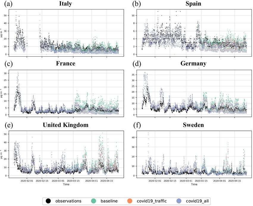
776                M. Guevara et al.: Time-resolved emission reductions for atmospheric chemistry modelling in Europe

Table 1. GNFR sector classification with the definition and sources of information used to derive emission reduction factors. The countries
considered for each sector are also listed.

  Sector       Description          Sources of information              Countries included
  GNFR_A       Energy industry      Electricity demand data:            Austria, Belgium, Bulgaria, Croatia, Czech Republic, Estonia,
                                    ENTSO-E (2020);                     France, Germany, Greece, Hungary, Ireland, Italy, Latvia, Lithua-
                                    FGC UES (2020)                      nia, Netherlands, Poland, Portugal, Romania, Slovakia, Slovenia,
                                    Outdoor temperature: C3S            Spain, Sweden, Switzerland, the UK, Russia
                                    (2017)
                                    Population map: CIESIN (2016)
  GNFR_B       Manufacturing        Electricity demand data:            Austria, Belgium, Bulgaria, Croatia, Czech Republic, Estonia,
               industry             ENTSO-E (2020);                     France, Germany, Greece, Hungary, Ireland, Italy, Latvia, Lithua-
                                    FGC UES (2020)                      nia, Netherlands, Poland, Portugal, Romania, Slovakia, Slovenia,
                                    Outdoor temperature: C3S            Spain, Sweden, Switzerland, the UK, Russia
                                    (2017)
                                    Population map: CIESIN (2016)
                                    Energy balances: Eurostat
                                    (2020a)
  GNFR_F       Road transport       Movement trend reports:             Austria, Belgium, Bulgaria, Croatia, Republic of Cyprus, Czech
                                    Google (2020)                       Republic, Denmark, Estonia, Finland, France, Germany, Greece,
                                                                        Hungary, Ireland, Italy, Latvia, Lithuania, Luxembourg, Malta,
                                                                        Netherlands, Poland, Portugal, Romania, Slovakia, Slovenia,
                                                                        Spain, Sweden, Switzerland, the UK, Turkey, Georgia, Bosnia
                                                                        and Herzegovina, Moldova, North Macedonia, Malta, Belarus
  GNFR_H       Aviation             Airport movement statistics:        Austria, Belgium, Bulgaria, Croatia, Republic of Cyprus, Czech
                                    FlightRadar (2020);                 Republic, Denmark, Estonia, Finland, France, Germany, Greece,
                                    Eurostat (2020b)                    Hungary, Ireland, Italy, Latvia, Lithuania, Luxembourg, Malta,
                                                                        Netherlands, Poland, Portugal, Romania, Slovakia, Slovenia,
                                                                        Spain, Sweden, Switzerland, the UK, North Macedonia, Norway

Table 2. Absolute [µg m−3 ] and relative changes [%] of modelled NO2 concentrations at urban and rural background stations (UB, RB) for
selected countries between 23 March and 26 April. The “N” column indicates the number of stations used to compute the changes.

               Country           Station       N    covid19_traffic –   covid19_all –    covid19_traffic –    covid19_all –
                                 type                  baseline (abs)   baseline (abs)     baseline (rel)     baseline (rel)
               IT (Milan)        UB            6               −17.1            −17.7         −54 %              −56 %
               ES (Madrid)       UB           19               −13.1            −14.9         −51 %              −58 %
               FR (Paris)        UB           16                −8.5            −11.0         −32 %              −41 %
               DE (Berlin)       UB            6                −2.9             −3.9         −23 %              −30 %
               GB (London)       UB            8                −7.4             −8.3         −25 %              −28 %
               SE (all)          UB            8                −0.9             −1.1         −10 %              −11 %
               IT                RB           69                −2.6             −2.7         −41 %              −43 %
               ES                RB           58                −0.7             −0.8         −28 %              −31 %
               FR                RB           23                −2.2             −2.3         −42 %              −44 %
               DE                RB           74                −1.9             −2.0         −26 %              −28 %
               GB                RB           14                −3.7             −4.0         −28 %              −30 %
               SE                RB            1                −0.5             −0.6         −11 %              −12 %

The following subsections describe the data and methods for             2.1   Energy industry
each sector along with the underlying assumptions.
                                                                        We assumed the changes in emissions from the energy in-
                                                                        dustry (which includes power and heat plants) to follow the
                                                                        changes observed in the electricity demand data reported by
                                                                        the European Network of Transmission System Operators

Atmos. Chem. Phys., 21, 773–797, 2021                                                        https://doi.org/10.5194/acp-21-773-2021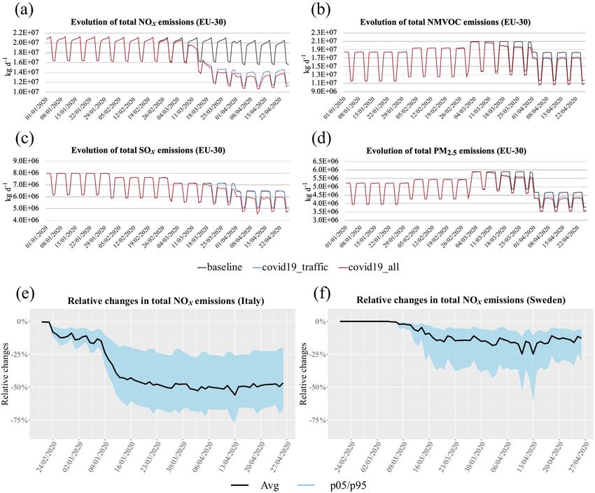
M. Guevara et al.: Time-resolved emission reductions for atmospheric chemistry modelling in Europe                           777

for Electricity (ENTSO-E) transparency platform (Hirth et         Each grid cell was assigned to a specific country following
al., 2018; ENTSO-E, 2020). ENTSO-E centralizes the col-           the global country mask available in the Emissions of atmo-
lection and publication of the electricity generation for each    spheric Compounds and Compilation of Ancillary Data sys-
European member state. For each country, we collected daily       tem (ECCAD, https://eccad.aeris-data.fr/, last access: Jan-
electricity demand data for the years 2015 to 2020 (January       uary 2021).
to April). Data gaps and inconsistencies found in the original       Julian day and day of week serve here as proxies for the
dataset were corrected using the electricity generation statis-   (climatological) main drivers of the seasonal and weekly
tics reported by the national transmission system operators       variability of the power demand, and the date index acts
(TSOs). For Russia, we derived the electricity demand data        as the trend term. We replicated the tuning strategy previ-
directly from Russia’s Federal Grid Company of Unified En-        ously used in Petetin et al. (2020) with a random search in
ergy System (FGC UES, 2020).                                      the hyper-parameter space and rolling-origin cross-validation
   In addition to its characteristic weekly variability, with     (appropriate for time series). While the training and tuning
higher values during weekdays, part of the electricity demand     of the GBM models were performed from 2015 to 2019, we
is driven by temperature fluctuations. Therefore, to calculate    used the first 2 months of 2020 (January–February) to test
the reduction in electricity demand during the COVID-19           the performance of the models.
lockdowns, we first estimated the business-as-usual (BAU)            Figure 2 summarizes the main statistics (normalized mean
electricity demand, i.e. the demand that would have occurred      bias, NMB; normalized root-mean-square error, NRMSE;
in the absence of lockdowns under the same meteorologi-           and correlation, r) obtained from the comparison between
cal conditions. To estimate the BAU electricity demand we         measured and ML-based electricity demand during the first
used machine learning models trained with meteorological          2 months of 2020 for selected countries. Generally, a high
data and other time features. This approach has been used         correlation (above 0.9) and low NMB and NRMSE (below
to weather-normalize NO2 surface concentration time series,       5 %) are observed for all cases, especially in those coun-
whose variability is also partly driven by the meteorologi-       tries with stronger lockdown restrictions such as Italy, France
cal conditions, to quantify actual reductions of NO2 during       or Spain. In this study, ML models are used for predicting
the COVID-19 lockdown (Petetin et al., 2020). More specif-        the fluctuations of electricity demand based on the temper-
ically, we used gradient boosting machine (GBM) models            ature (and additional time features), assuming that temper-
trained and tuned independently for each country using daily      ature is a strong driver of electricity demand (for heating
data from January to April between 2015 and 2019. As in-          and air conditioning). However, temperature is obviously not
puts, we considered the following features: daily country-        the only driver of electricity demand variability that can be
level population-weighted heating degree days (HDDs), date        influenced by various other factors (e.g. change of technol-
index (number of days since 1 January 2015), Julian date,         ogy, behaviour, regulation). In addition, the GBM models
day of week and a Boolean feature indicating the country-         used in this study are non-parametric, meaning that they can-
specific bank holidays. The HDD is defined relative to a          not extrapolate, i.e. predict electricity demand values out-
threshold temperature (Tb ) above which a building needs          side the range of values used during the training phase. As
no heating and is used to approximate the daily energy de-        a consequence, such models may perform poorly when an
mand for heating a building (Quayle and Diaz, 1980). In           overly strong trend and/or inter-annual variability (not di-
order to provide a more realistic estimate of the potential       rectly due to temperature variability) are affecting the elec-
electricity demand for space heating on a national level, we      tricity demand to predict. In practise, the results obtained in
computed country-specific population-weighted HDD values          this study show that this approach performs relatively well
(HDD_pop(d)) following Eq. (1):                                   in most countries, although there are some exceptions. The
                                                                  poorest performance was obtained in Finland (r = 0.33), due
                n
                X (max(Tb − T2 m (x, d), 0)) × Pop(x)             to a strong negative anomaly (−12 % on average) of elec-
HDD_pop(d) =                     n                      ,   (1)
                x=1
                                 P                                tricity demand in January–February 2020 compared to pre-
                                      Pop(x)
                                x=1                               vious years used for training. As shown in Fig. S1 in the
                                                                  Supplement, the electricity demand reported by ENTSO-E
where T2 m (x, d) is the daily mean 2 m outdoor temperature       for this country in early 2020 (i.e. late January–early Febru-
for grid cell x and day d [◦ C], Pop(x) is the amount of pop-     ary) was substantially lower than during all previous years
ulation included in grid cell x [no. of inhabitants] and n is     (2015–2019). However, this anomaly in the power data can-
the total number of grid cells that corresponds to a specific     not be explained by a drastic change in the temperature, as
country. A threshold temperature value of 15.5 ◦ C was se-        this parameter remained within the same range of values as
lected following Spinoni et al. (2015). Outdoor temperature       during previous years. In such a situation, where changes in
information was obtained from the ERA5 reanalysis dataset         power demand cannot be related to changes in temperature,
for the period 2015–2020 (C3S, 2017), while information           the ML cannot produce accurate predictions. Compared to
on gridded population was derived from the Gridded Pop-           most other countries, a larger NRMSE and lower correlation
ulation of the World, Version 4 (GPWv4; CIESIN, 2016).            were also found in Luxembourg. In this case, we attribute the

https://doi.org/10.5194/acp-21-773-2021                                              Atmos. Chem. Phys., 21, 773–797, 2021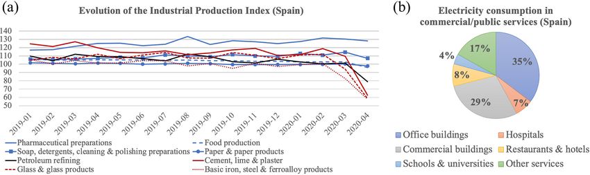
778                M. Guevara et al.: Time-resolved emission reductions for atmospheric chemistry modelling in Europe

Figure 2. Summary of the statistics (normalized mean bias, NMB; normalized root-mean-square error, NRMSE; and correlation, r) obtained
from the comparison between measured and computed electricity demand during the first 2 months of 2020 for selected countries.

low performance of the ML algorithm to the large data gap            of the electricity production in these countries comes from
found in the historical data used for training. For instance, for    renewable energy sources. For instance, in the case of Nor-
the year 2019 the ENTSO-E dataset presents a temporal cov-           way more than 90 % of the electricity production comes from
erage lower than 50 %. In addition, despite relatively good          hydropower (IEA, 2020a)
statistics in early 2020, the electricity demand computed in            The electricity demand started to decrease by the end of
Denmark and Norway shows a substantial and unexpected                February and the beginning of March 2020 compared to the
increase during the COVID-19 lockdown (up to +12 %). In              BAU electricity demand estimated from the GBM models in
the case of Denmark, we found higher-than-usual electric-            countries where strong restrictions had been implemented.
ity demand levels reported by ENTSO-E in late February–              We attributed these discrepancies to the direct effect of lock-
early March 2020 which, as in the case of Finland, could             down measures, regardless of the meteorological conditions,
not be directly explained by drastic changes in temperature          and used them to derive quantitative daily emission reduction
(Fig. S2). At this time of the year, such relatively high-power      factors for the energy industry sector (Eq. 2):
demand was already observed in 2018 but because of strong
cold waves, while temperature was not particularly cold in           RFener_indu (d, c)
2020. Like in the case of Finland, unexplained changes in
                                                                         EDCOVID-19 (d, c) − EDmeasured (d, c)

the electricity demand induce errors in the predictive ML al-        =                                           × 100,           (2)
                                                                                      EDmeasured (d, c)
gorithm. For Norway, although the mean bias on the entire
test period is relatively low, a closer look at the time series      where RFener_indu (d, c) is the final reduction factor for
indicates that this bias was low at the beginning of the period      the energy industry sector for day d and country c [%],
and started to increase in mid-February and persisted during         EDCOVID-19 (d, c) is the estimated BAU electricity demand
the lockdown (Fig. S3). Therefore, it is unclear to which ex-        computed using ML for day d and country c [MW], and
tent the increase in electricity demand during the lockdown is       EDmeasured (d, c) is the measured electricity demand for day
real or simply the persistence of the bias previously observed       d and country c [MW].
before the lockdown starts (as both are of the same order of            Figure 3a illustrates the reduction factor trends obtained
magnitude). Without additional sources of information and            for selected countries. As expected, the strong weekly cy-
given the relatively soft mobility restrictions imposed in Nor-      cle of electricity demand normally observed in most coun-
way, we also discarded the use of ML for this country and            tries smoothed down during the COVID-19 lockdown. The
assumed that electricity demand during the lockdown period           resulting trends are consistent with the national lockdown
was not significantly impacted.                                      calendars and restriction levels implemented in each coun-
   Considering all of the above, and as a precautionary mea-         try. Italy is the first country where traffic activity reductions
sure, we assumed a null reduction of the electricity demand          happened, followed by Spain, France, Germany, the UK and
in Denmark, Finland and Norway and a fixed −16 % reduc-              Sweden. This is in line with the starting dates of lockdown
tion in Luxembourg starting the first day of the national lock-      restrictions in each country (Sect. 2). For Spain, reduction in-
down implementation (15 March), following the results re-            creased between 30 March and 9 April, the most restrictive
ported by Le Quéré et al. (2020). Importantly, we do not ex-         phase of the Spanish lockdown when only essential activities
pect that assuming a null reduction will cause a significant         including food trade, pharmacy and some industries were au-
impact on the computed emission reductions, as the majority          thorized. In the case of Sweden, positive values are observed

Atmos. Chem. Phys., 21, 773–797, 2021                                                    https://doi.org/10.5194/acp-21-773-2021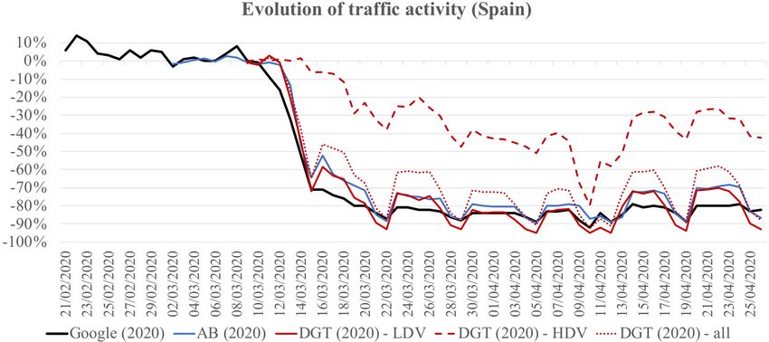
M. Guevara et al.: Time-resolved emission reductions for atmospheric chemistry modelling in Europe                                    779

Figure 3. Emission reduction factors computed for the energy (a) and manufacturing (b) industries, road transport (c), and aviation (d) for
selected countries (IT, Italy; ES, Spain; FR, France; DE, Germany; GB, Great Britain; SE, Sweden) for the period 21 February to 26 April
2020. Original and COVID-19 version of the emission daily temporal factors computed for the road transport sector and used for emission
modelling (e).

for certain days until the beginning of April. These results            of the population may have increased household electricity
agree with the ones reported in Le Quéré et al. (2020), who             consumption. During the strictest period of the COVID-19
obtained a 4 % increase during the lockdown for this country.           lockdown (23 March–26 April), Italy was the country expe-
It is likely that electricity demand from public and commer-            riencing the largest reductions (−21 %), followed by Spain
cial services remained unperturbed as, in contrast to most              (−15 %) and France (−14.4 %).
countries, there was no enforced lockdown in Sweden. We                    The countries for which daily reduction factors could be
also hypothesize that a voluntary self-isolation of a fraction          computed are shown in Table 1. For countries with no data,

https://doi.org/10.5194/acp-21-773-2021                                                      Atmos. Chem. Phys., 21, 773–797, 2021
780                M. Guevara et al.: Time-resolved emission reductions for atmospheric chemistry modelling in Europe

Figure 4. Evolution of the industrial production index in Spain for selected manufacturing industrial branches between January 2019 and
April 2020 (INE, 2020) (a). Contribution of each commercial and public service branch to total electricity consumption in Spain for 2017
(IDAE, 2018) (b).

we constructed a set of reduction factors based on the aver-          cial buildings, schools, universities, restaurants and hotels,
age data of all the available countries except Italy, where the       which represent more than 70 % of the total electricity con-
lockdown restrictions began approximately 3+ weeks before             sumption, were obliged, in most cases, to close their facilities
other countries.                                                      during the lockdown.
                                                                         The reduction of power demand attributable to the manu-
2.2   Manufacturing industry                                          facturing industry sector was then translated into a total re-
                                                                      duction in industrial activity using the national energy bal-
The reduction factors for manufacturing industry are based            ances reported in Eurostat (2020a) (Eq. 3):
on the daily electricity demand reduction factors described
                                                                                              RFeneindu (d, c) × 0.25
in Sect. 2.1. We attributed 25 % of the total electricity de-         RFmanuf_indu (d, c) =                           ,             (3)
mand reduction to the reduction in manufacturing industry                                            Sindu (c)
activity, which is consistent with the −27 % decrease in elec-        where RFmanuf_indu (d, c) is the final reduction factor for the
tricity use by the manufacturing sector reported by the elec-         manufacturing industry sector for day d and country c [%],
tricity transmission system operator of France (RTE, 2020).           RFeneindu (d, c) is the reduction factor for the total electric-
We estimated this value considering that (i) the European in-         ity demand for day d and country c estimated as described
dustry sector consumes 22.3 % of the total final electricity          in Sect. 2.1 [%], and Sindu (c) is the share of final electricity
demand (Eurostat, 2020a) and (ii) most of the electricity re-         consumed by the industrial sector in country c [%] (Eurostat,
duction during the lockdown can be linked to commercial               2020a).
and public services. Indeed, those industrial branches respon-           Figure 3b shows the daily reduction factors computed for
sible for manufacturing essential goods (e.g. food, pharma-           selected countries. The original positive values (i.e. increase
ceutical preparations and other chemical products) remained           in electricity consumption) obtained for the energy industry
almost unaffected during the COVID-19 lockdowns, in con-              sector (Fig. 3b) were replaced by zeros for the calculations,
trast to the commercial and public services sectors, which            as we consider it unlikely that average increases in manufac-
were forced to drastically reduce or even completely halt             turing industrial emissions occurred during the lockdown. In
their activities (i.e. restaurants and hotels, office buildings,      general, the trends observed in all countries follow the same
shopping centres). This fact is illustrated in Fig. 4 which           pattern as the ones presented for the energy industry. During
shows, on the one hand, the evolution of the industrial pro-          the strictest period of the COVID-19 lockdown, computed
duction index (IPI) for selected industrial branches in Spain         reductions are between −13 % and −10 % for Italy, Spain,
between January 2019 and April 2020 (INE, 2020) and, on               France and the UK, −4 % for Germany; and −0.8 % for Swe-
the other hand, the contribution of each Spanish commercial           den.
and public service branch to the total electricity consump-
tion (IDAE, 2018). While certain industrial branches suffered         2.3   Road transport
important decreases in their production levels in March and
April 2020 (i.e. production of mineral products, steel indus-         The emission reduction factors considered for the road trans-
try), the essential ones kept about the same level of productiv-      port sector are based on the Google COVID-19 Commu-
ity (i.e. pharmaceutical preparations, manufacturing of soap          nity Mobility Reports (Google LLC, 2020). The Google
and detergents, food and paper production, and, to a lesser           dataset reports daily movement trends over time by geogra-
extent, petroleum refining). In contrast, office and commer-          phy (country and region) across different categories of places

Atmos. Chem. Phys., 21, 773–797, 2021                                                     https://doi.org/10.5194/acp-21-773-2021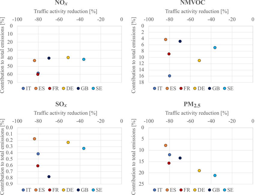
M. Guevara et al.: Time-resolved emission reductions for atmospheric chemistry modelling in Europe                                   781

Figure 5. Comparison of traffic movement trends for Spain derived from Google reports (Google, 2020) and measured traffic counts in the
city of Barcelona (ATM, personal communication) and the main Spanish interurban roads (DGT, 2020), the latter one being also distinguished
by type of vehicle (i.e. light-duty vehicles, LDVs; heavy-duty vehicles, HDVs).

(i.e. groceries and pharmacies, parks, transit stations, retail        light- and heavy-duty vehicles when developing the reduc-
and recreation, residential and workplaces) based on aggre-            tion factors because CAMS-REG_AP/GHG traffic-related
gated and anonymized sets of data from users who have                  emissions are not discriminated by type of vehicle. Conse-
turned on the “location history” setting for their Google ac-          quently, our factors for the traffic sector may overestimate
count on their mobile devices. For the present study, we used          the overall reduction of emissions, especially in areas with
the mobility trends reported for the transit station category,         a higher share of heavy-duty vehicles, typically interurban
which includes places like public transport hubs such as sub-          roads. In order to quantify this uncertainty, we used the Span-
ways, bus and train stations. The assumption behind this               ish official EMEP road transport emissions (EMEP/CEIP,
choice is that movement trends observed in public transport            2021) which, unlike CAMS-REG-AP, are reported by vehi-
hotspots correlate with private transport trends. Reductions           cle category, to quantify the impact of omitting the distinc-
for each day are calculated by Google from a baseline taken            tion between light- and heavy-duty vehicles when developing
as the median value, for the corresponding day of the week,            the reduction factors. We compared the NOx average emis-
over a 5-week period prior to the lockdowns (3 January to              sion reductions obtained for the road transport sector during
6 February).                                                           the strictest lockdown period (23 March to 26 April) when
   We evaluated the Google movement trends with actual                 considering the DGT (2020) trends for heavy-duty vehicles
measured traffic counts from the city of Barcelona (ATM,               instead of the Google movement trends. Results indicate a
personal communication) and other major interurban roads               −18 % difference between the computed average reductions,
in Spain (DGT, 2020), the latter discriminated by vehi-                i.e. −528.5 t when using Google trends for all vehicle cat-
cle type (light and heavy duty) (Fig. 5). Note that for the            egories and −434.4 t when considering specific heavy-duty
Barcelona and DGT data, the information is available from 3            vehicle trends (Fig. S4). This difference may vary across
and 9 March onwards, respectively. In general terms, Google            countries due to differences in (i) the impact of COVID-19
data reproduce the measurement-based trends obtained for               restriction on the activity of heavy-duty vehicles and (ii) the
the city of Barcelona (BCN) and the Spanish interurban                 contribution of the heavy-duty vehicles to the overall traffic
roads (DGT-all), with correlations of 0.96 and 0.92, respec-           emissions. This approach may be improved in the future but
tively. Overall, the average reductions reported by each of            was constrained in this study by data availability.
these three datasets are similar: −74.6 % (Google), −69.1 %               Figure 3c shows the reduction factors proposed for se-
(BCN) and −63.62 % (DGT-all). Using Google data at tran-               lected countries. As in the case of the energy industry, the re-
sit stations tends to slightly overestimate the reductions ob-         sulting trends are in line with the implementation and evolu-
served during the weekdays. However large discrepancies are            tion of the national restrictions imposed in each country. The
shown when comparing the Google trend against the one re-              decrease in the traffic activity in Italy starts 2 d after the im-
ported by DGT for heavy-duty vehicles (DGT-heavy). The                 plementation of the localized lockdown and intensified once
data from the DGT report an average reduction of heavy-                the national lockdown was imposed on 12 March, reaching
duty vehicles of only −31 % (more than 2 times lower than              reductions of about −80 %. In the case of Spain and France,
the one reported by Google), as these vehicles supported the           similar traffic reduction levels were reached just 3 d after the
delivery of essential goods and products (e.g. food, medical           beginning of the corresponding national lockdowns. For the
supplies). Nevertheless, we omitted the distinction between            UK and Germany, the largest reductions are around −70 %

https://doi.org/10.5194/acp-21-773-2021                                                     Atmos. Chem. Phys., 21, 773–797, 2021
782                M. Guevara et al.: Time-resolved emission reductions for atmospheric chemistry modelling in Europe

and −50 %, respectively. The lower reductions in Sweden           scale Online Nonhydrostatic AtmospheRe CHemistry model
(around −40 %) are consistent with the lack of enforced mo-       (MONARCH) (see Sect. 3.1) and the High-Elective Reso-
bility restrictions in this country at any point. In all cases,   lution Modelling Emission System version 3 (HERMESv3)
the activity started recovering during the last week of the pe-   (Sect. 3.2) both developed at the Barcelona Supercomput-
riod of study, coinciding with the relaxation of the mobility     ing Center. The simulation period for the case study is from
restrictions.                                                     20 January to 26 April 2020. The study period covers 1
   The list of countries included for this sector is summa-       month of pre-COVID lockdown conditions (the first local-
rized in Table 1. For countries without available data we         ized lockdowns in Europe began on 21 February in the re-
constructed a set of average reduction factors considering all    gion of Lombardy) and more than 2 months of lockdown
countries except Italy.                                           conditions, including 5 weeks (23 March to 26 April) during
                                                                  which the most severe restrictions were already implemented
2.4    Aviation                                                   in most (22) European countries. Therefore, the selected pe-
                                                                  riod of study allows analysis of the changes in concentrations
We derived the reduction factors related to air traffic emis-     between the lockdown period and before.
sions during landing and take-off (LTO) cycles in airports           Three air quality simulations were run: (i) using the de-
from statistics provided by FlightRadar24 (FlighRadar24,          fault CAMS-REG-APv3.1 emissions without considering
2020), which reports, every day, the total number of tracked      any emission reduction, hereafter referred to as the baseline
operations per airport over the preceding 30 d. For each coun-    scenario; (ii) considering the traffic-related emission reduc-
try, we selected the largest airport to represent a national      tion factors only, hereafter referred to as the covid19_traffic
proxy. We computed country-specific daily flight operation        scenario; and (iii) including the reduction factors from the
trends using as a baseline value the average number of oper-      traffic, energy and manufacturing industries and aviation sec-
ations per airport from the previous year reported by Eurostat    tors, hereafter referred to as the covid19_all scenario. The
statistics (Eurostat, 2020b).                                     base year of the CAMS-REG-APv3.1 emissions used in the
    We started collecting the information from FlightRadar24      three scenarios is 2016, which was the most recent year avail-
for all airports on 6 March, and the information from previ-      able at the time of the study.
ous dates could not be retrieved as it is not archived. There-       We also compared the model results against measure-
fore, our reduction factors have as an initial date 6 March       ments of the European Environmental Agency (EEA) AQ e-
in all cases, independently of the lockdown calendars. As         Reporting (EEA, 2020) available through the Globally Har-
shown in Fig. 3d for most countries the reductions in flight      monised Observational Surface Treatment (GHOST) project
activity were starting to occur during those dates and there-     (Sect. 3.3). The model and evaluation work focus on NO2 .
fore the trends presented are consistent. However, in some        Given that our main focus is the emission reductions and
other countries such as Italy, reductions were already in a       their evaluation, the inclusion of other relevant yet more
more advanced state (first day of reduction is −15 %). We         model-dependent secondary pollutants such as O3 or PM2.5
do not expect this lack of information to significantly affect    is beyond the scope of this paper. The impact of the lockdown
the emission and air quality modelling results, as the contri-    upon secondary pollutants, which are affected by more com-
bution of this pollutant sector to total European emissions is    plex chemical interactions and source contributions, may be
very low, i.e. 1.1 % and 0.14 % to total NOx and PM10 emis-       addressed in a follow-up multi-model study.
sions, according to the last available EMEP official reported
emission data (EMEP/CEIP, 2021). We expect to comple-             3.1   MONARCH model
ment this information from alternative sources of data in a
future release of the dataset. Regarding the obtained results,    MONARCH v1.0 (Pérez et al., 2011; Haustein et al., 2012;
it is observed that in almost all countries, the reduction lev-   Jorba et al., 2012; Spada et al., 2013; Badia and Jorba,
els reached values of −90 % or more before the beginning          2015; Badia et al., 2017) is a fully online integrated sys-
of April. In contrast to road transport, there were no signs      tem for meso-scale to global-scale applications developed at
of recovery during the last week of April for this sector, as     the Barcelona Supercomputing Center (BSC). A flexible gas-
the movements between countries were still restricted at that     phase module combined with a hybrid sectional-bulk mul-
time.                                                             ticomponent mass-based aerosol module is implemented in
                                                                  the MONARCH model, which uses the Nonhydrostatic Mul-
                                                                  tiscale Model on the B-grid (NMMB; Janjic and Gall, 2012)
3     Evaluating the reduction factors with air quality           as the meteorological core driver. The Carbon Bond 2005
      modelling                                                   chemical mechanism (CB05; Yarwood et al., 2005) extended
                                                                  with toluene and chlorine chemistry is the gas-phase scheme
We performed an emission and air quality modelling study          used in MONARCH. The CB05 is well formulated for ur-
as a first demonstration and evaluation of the applicability of   ban to remote tropospheric conditions and it considers 51
the developed emission reduction factors. We used the Multi-      chemical species and solves 156 reactions. The rate con-

Atmos. Chem. Phys., 21, 773–797, 2021                                                https://doi.org/10.5194/acp-21-773-2021
M. Guevara et al.: Time-resolved emission reductions for atmospheric chemistry modelling in Europe 783
stants were updated based on evaluations from Atkinson et gaseous and aerosol emissions for use in atmospheric chem-
al. (2004) and Sander et al. (2006). The photolysis scheme istry models (Guevara et al., 2019). The HERMESv3 sys-
used is the Fast-J scheme (Wild et al., 2000). It is coupled tem was used to remap the original CAMS-REG-AP data
with physics of each model layer (e.g. aerosols, clouds, ab- (0.1◦ × 0.05◦ ) onto the MONARCH modelling domain and
sorbers as ozone) and it considers grid-scale clouds from the to derive hourly and speciated emissions. Aggregated annual
atmospheric driver. The Fast-J scheme has been updated with emissions were broken down into hourly resolution using the
CB05 photolytic reactions. The quantum yields and cross emission temporal profiles reported by Denier van der Gon
section for the CB05 photolysis reactions have been revised et al. (2011). The speciation of NMVOCs and PM emissions
and updated following the recommendations of Atkinson et was performed using the split factors reported by TNO (Kue-
al. (2004) and Sander et al. (2006). The aerosol module in nen et al., 2014).
MONARCH describes the life cycle of dust, sea salt, black For the covid19_traffic and covid19_all scenarios, the esti-
carbon, organic matter (both primary and secondary), sul- mated reduction factors (Fig. 3a–d) were combined with the
fate and nitrate aerosols. While a sectional approach is used original temporal profiles in order to model dynamic emis-
for dust and sea salt, a bulk description of the other aerosol sion reductions for each sector and country. For each pol-
species is adopted. A simplified gas–aqueous–aerosol mech- lutant sector, we constructed a dataset of country-specific
anism has been introduced in the module to account for COVID-19 daily temporal profiles by combining the origi-
the sulfur chemistry, the production of secondary nitrate- nal temporal weight factors reported by Denier van der Gon
and ammonium-containing aerosols is solved using the ther- et al. (2011) with the computed emission reduction factors,
modynamic equilibrium model EQSAM, and a two-product following Eq. (4):
scheme is used for the formation of secondary organic
aerosols from biogenic gas-phase precursors. Meteorology- RFs (c, d)
DF_covid19s (c, d) = DFs (d) × 1 + , (4)
driven emissions are computed within MONARCH. Min- 100
eral dust emissions are calculated with an updated version
of the Pérez et al. (2011) scheme, the sea salt aerosol emis- where DFs (d) represents the daily temporal factors for pollu-
sions following Jaeglé et al. (2011) and biogenic gas-phase tant source s and day of the year d [0 to 366], and RFs (c, d) is
species using the MEGANv2.04 model (Guenther et al., the reduction factor computed for sector s, day of the year d
2006). The model provides operational regional mineral dust and country c [%]. The DFs (d) weight factors were obtained
forecasts for the World Meteorological Organization (WMO; by combining the original monthly (January to December)
https://dust.aemet.es/, last access: January 2021) and partici- and weekly (Monday to Sunday) temporal profiles reported
pates in the WMO Sand and Dust Storm Warning Advisory by Denier van der Gon et al. (2011). Figure 3e illustrates the
and Assessment System for Northern Africa-Middle East- COVID-19 daily temporal factors for the road transport sec-
Europe (http://sds-was.aemet.es/, last access: January 2021). tor in selected countries. The original daily profile for this
Since 2012, the system has contributed with global aerosol sector, which is used in the baseline scenario, is also plot-
forecasts to the multi-model ensemble of the ICAP initia- ted for comparison purposes. In general, the temporal disag-
tive (Xian et al., 2019), and since 2019, it has been a candi- gregation of emissions would require the sum of the daily
date model of the CAMS – Air Quality Regional Production weight factors to be 366 (as in this case the year of study is
(Marecal et al., 2015). a leap year). Nevertheless, and due to the application of the
In this work, the model is configured for a regional domain reduction factors, the sum of the COVID-19 daily factors do
covering Europe and part of northern Africa. The rotated lat– not add up to this number, which allows simulation of time-
long projection is used, with a regular horizontal grid spac- resolved emission reductions.
ing of 0.2◦ , and the top of the atmosphere is set at 50 hPa
3.3 Observational dataset
using 48 vertical layers. Figure S1 displays the domain of
study. Meteorological initial and boundary conditions were The GHOST project is a BSC initiative dedicated to the har-
obtained from the ECMWF global model forecasts at 0.125◦ monization of publicly available global surface observations
and chemical boundary conditions from the CAMS global (most notably air quality pollutants) and metadata, for the
model forecasts at 0.4◦ (Flemming et al., 2015). For an effi- purpose of facilitating a greater quality of observational–
cient execution of the modelling chain, the autosubmit work- model comparison in the atmospheric chemistry community
flow manager is used (Manubens-Gil et al., 2016). (Bowdalo et al., 2020). Numerous networks are currently
processed and contained under the umbrella of GHOST, in-
3.2 HERMESv3 emission system cluding, among others, the EBAS and EEA networks. For
each network, all relevant numerical and textual metadata
The original annual CAMS-REG-APv3.1 emission inven- (e.g. station classifications, measurement methodologies) are
tory was processed using the HERMESv3 system, an open- standardized and all data are passed through numerous qual-
source, stand-alone multi-scale atmospheric emission mod- ity control tests, giving detailed quality assurance (QA) flags.
elling framework developed at the BSC that computes
https://doi.org/10.5194/acp-21-773-2021 Atmos. Chem. Phys., 21, 773–797, 2021784 M. Guevara et al.: Time-resolved emission reductions for atmospheric chemistry modelling in Europe
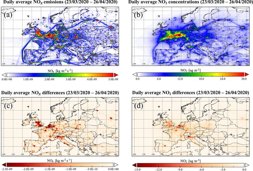
Figure 6. Maps of the daily average NOx emissions [kg s−1 m−2 ] (a) and NO2 concentrations [µg m−3 ] (b) obtained for the baseline
scenario (23 March to 26 April) and differences (c, d) when compared to the covid19_all scenario (i.e. covid19_all minus baseline). The
spatial resolution of all maps is 0.2◦ × 0.2◦ .
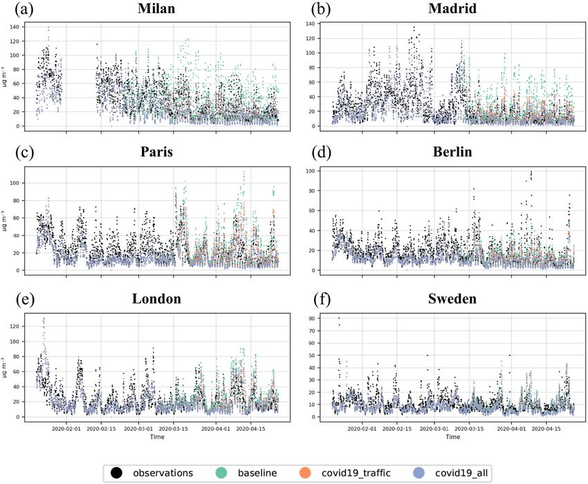
In this work, we used the NO2 near-real-time EEA data. puted results. A detailed description of the stations is avail-
We selected rural and urban background stations located at able in Table S1 in the Supplement and Fig. S5.
selected countries (Italy, Spain, France, Germany, the UK
and Sweden). In the case of urban background stations, we
selected those located in Milan, Madrid, Paris, Berlin and 4 Results and discussion
London. For Sweden, and due to the low density of stations
found in individual cities (e.g. Stockholm, one station), we Figure 6 shows maps of daily average NOx emissions
decided to consider all urban background stations available [kg s−1 m−2 ] and NO2 concentrations [µg m−3 ] obtained for
countrywise (six). GHOST provides a wide range of harmo- the baseline scenario between 23 March and 26 April, as well
nized metadata and quality assurance (QA) flags for all pol- as the differences with respect to the covid19_all scenario
lutant measurements. In this study, we took benefit of these (i.e. covid19_all minus baseline). During this 5-week period
flags to apply an exhaustive QA screening. More details on most European countries were under severe national lock-
the QA flags used can be found in Appendix A. Note that down restrictions, which allows the illustration of the largest
for Italy, there is a data gap between 1 and 13 February at impacts upon emissions and air quality levels.
all stations. We nevertheless decided to keep this country in For both NOx emissions and NO2 concentrations, the main
our evaluation study since it is one of the European countries reductions occurred in urban areas and the main interurban
most affected by the COVID-19 pandemic and the data gap roads, especially within the most affected countries (i.e. Italy,
does not affect the lockdown period. In the case of Sweden, Spain, France, the UK). The largest emission reductions are
only one rural background station was available for the entire related to traffic (Sect. 4.1), which is the main contributor
country, which may reduce the representativity of the com- to urban NO2 levels, with approximately a 40 % share on
average (EEA, 2019). Below we discuss the results obtained
Atmos. Chem. Phys., 21, 773–797, 2021 https://doi.org/10.5194/acp-21-773-2021M. Guevara et al.: Time-resolved emission reductions for atmospheric chemistry modelling in Europe 785
from the modelling experiments in terms of daily changes port and energy industry (Fig. 3a and c). The daily variability
in emissions (Sect. 4.1) and NO2 air quality concentrations of the reduction factors for road transport is generally low; in
(Sect. 4.2) during the study period. the case of the energy industry large day-to-day variations
are observed.
4.1 Emissions Despite having experienced one of the largest reductions
in road transport activity (more than −80 %), Spain was
Figure 7a–d shows the evolution of daily NOx , NMVOCs, the country with the lowest decrease in total PM2.5 emis-
SOx and PM2.5 emissions during the entire period of study sions (−4.3 %), and the second lowest in terms of NMVOCs
(20 January to 26 April) for EU-30 and for each of the three (−4.4 %). Sweden shows a PM2.5 emission reduction of
scenarios. The largest emission reductions occurred during −7.6 %, almost 2 times larger than Spain and very close to
the second and third weeks of March, when several European Italy (−9.2 %), despite its lower traffic activity decrease (less
countries enforced national lockdown restrictions. After this than −40 %). This is explained by the different contributions
period, there was a stabilization of the emission reductions of the road transport sector contribution to total emissions
until approximately 19 April. Thereafter, a slight recovery in each country. Figure 9 shows the relationship between the
of the emission levels started to occur, which is consistent reduction of traffic activity and contribution of the road trans-
with the recovery of traffic activity shown in Fig. 3c. Overall, port sector to total emissions per country and pollutant. In the
and when comparing the baseline and covid19_all scenarios, case of Sweden, road transport represents around 21.3 % of
the reduction of total emissions is −33 % for NOx , −8 % for total PM2.5 emissions, while in Spain the contribution is just
NMVOCs, −7 % for SOx and −7 % for PM2.5 . The contri- 7.9 %. Similarly, in the case of NMVOCs emissions the con-
bution of the traffic sector to total reductions is especially tribution of road transport emissions is 15.9 % in Italy and
relevant for NOx (90 %), NMVOCs (87 %) and PM2.5 (82 %) 8.9 % in France, while in Spain it is only 4.3 %.
while for SOx most of the total reduction can be attributed
to the decreases in the energy and manufacturing industries 4.2 Air quality
(97 %), according to the results shown by the covid19_traffic
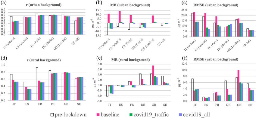
scenario. Figure 7e and f illustrate the average and 5th and Figure 10 shows the observed and modelled hourly NO2
95th percentiles (p05, p95) of the daily relative changes [%] concentrations between 20 January and 26 April at selected
in the gridded NOx emissions for Italy and Sweden. The re- urban background sites in Italy (Milan), Spain (Madrid),
sults were computed considering all the grid cells within each France (Paris), the UK (London), Germany (Düsseldorf) and
of the countries. In Italy, the last 2 weeks of March and first 2 Sweden (all available sites). In the same way, the results
weeks of April show certain areas of the country reaching re- at rural background stations are presented in Fig. 11. In
ductions up to −75 %, whereas in other areas less affected by both cases, the results are presented separately for each of
anthropogenic (and particularly road transport) emissions the the emission scenarios considered: baseline (in magenta),
reductions were significantly lower (∼ −25 %). In the case covid19_traffic (in green) and covid19_all (in blue). Statis-
of Sweden, the reductions ranged between −6 % (p95) and tical parameters computed on an hourly basis (i.e. mean bias,
−36 % (p05). MB; root-mean-square error, RMSE; correlation coefficient,
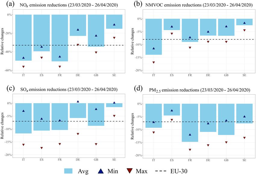
Figure 8 summarizes the average, minimum and max- r) are presented for each emission scenario, country and sta-
imum national daily emission changes [%] obtained for tion type for the pre-lockdown (20 January to 20 February)
NOx , NMVOCs, SOx and PM2.5 between 23 March and and most restrictive lockdown periods (23 March to 26 April)
26 April for selected countries along with the average (Fig. 12). For the pre-lockdown period, the calculated statis-
at the EU-30 level. Changes in emissions present strong tics are equal for all scenarios, as no emission reductions are
variations from country to country and pollutant to pollu- considered during that time. The computation of statistics
tant. For NOx and SOx , all countries except Germany and during the pre-lockdown period allows quantification of the
Sweden present stronger average reductions than the ones performance of the system under BAU conditions. We also
reported at the EU-30 level (−33 % and −7 %, respec- compare the observed and simulated NO2 decline from the
tively), and Italy and France are the two countries with the pre-lockdown to lockdown periods in each region, to quan-
largest reductions (−50 % for NOx and −12 % for SOx ). tify the accuracy of the estimated emission reduction factors
For NOx , minimum and maximum daily emission reduc- (Fig. 13). Finally, Table 2 summarizes the absolute and rela-
tions are in general relatively close to the average (e.g. tive changes of NO2 concentrations modelled at each station
Italy: avg = −50 %, min = −47 % and max = −56 %; Spain: type and country between 23 March and 26 April.
avg = −40 %, min = −43 % and max = −46 %). In contrast, The MONARCH model is capable of reproducing
there are large differences among the average, minimum and the urban background NO2 observations during the
maximum daily SOx changes, especially in Germany (Swe- pre-lockdown period fairly well, particularly in Lon-
den) where changes in emissions go from 0.6 % (0.15 %) to don (MB = −0.25 µg m−3 , RMSE = 16 µg m−3 , r = 0.74),
−12 % (−5 %). The different behaviours observed for NOx Madrid (MB = −4 µg m−3 , RMSE = 19 µg m−3 , r = 0.64)
and SOx are related to the different trends of the road trans- and Paris (MB = −7.7 µg m−3 , RMSE = 13 µg m−3 , r =
https://doi.org/10.5194/acp-21-773-2021 Atmos. Chem. Phys., 21, 773–797, 2021You can also read