Predicting power outages caused by extratropical storms
←
→
Page content transcription
If your browser does not render page correctly, please read the page content below
Nat. Hazards Earth Syst. Sci., 21, 607–627, 2021
https://doi.org/10.5194/nhess-21-607-2021
© Author(s) 2021. This work is distributed under
the Creative Commons Attribution 4.0 License.

Predicting power outages caused by extratropical storms
Roope Tervo1, , Ilona Láng1, , Alexander Jung2 , and Antti Mäkelä1
1 FinnishMeteorological Institute, B.O. 503, 00101 Helsinki, Finland
2 Aalto
      University, Department of Computer Science, B.O. 11000, 00076 Aalto, Finland
 These authors contributed equally to this work.

Correspondence: Roope Tervo (roope.tervo@fmi.fi)

Received: 22 June 2020 – Discussion started: 3 August 2020
Revised: 30 October 2020 – Accepted: 7 January 2021 – Published: 11 February 2021

Abstract. Strong winds induced by extratropical storms            a significant risk for the power supply in Finland, which
cause a large number of power outages, especially in highly       has over 90 000 km of overhead lines (70 % are part of the
forested countries such as Finland. Thus, predicting the im-      medium-voltage, 1–35 kV, network) passing through forest
pact of the storms is one of the key challenges for power         (Kufeoglu and Lehtonen, 2015). Between the years 2010
grid operators. This article introduces a novel method to pre-    and 2018, on average 46 % of all transmission faults in Fin-
dict the storm severity for the power grid employing ERA5         land were caused by extratropical storms (Finnish Energy,
reanalysis data combined with forest inventory. We start by       2010–2018). During the years of the most damaging storms,
identifying storm objects from wind gust and pressure fields      2011 and 2013, the share of windstorm damage of all fault
by using contour lines of 15 m s−1 and 1000 hPa, respec-          causes was up to 69 % (Finnish Energy, 2011, 2013). The
tively. The storm objects are then tracked and characterized      need for managing power interruptions is even more urgent
with features derived from surface weather parameters and         since the power suppliers in Finland are obliged to finan-
forest vegetation information. Finally, objects are classified    cially compensate customers of urban areas after 6 h and ru-
with a supervised machine-learning method based on how            ral areas after 36 h of interruption in electricity distribution
much damage to the power grid they are expected to cause.         (Nurmi et al., 2019). Thus they require a large workforce to
Random forest classifiers, support vector classifiers, naïve      fix caused damage rapidly.
Bayes processes, Gaussian processes, and multilayer percep-          As Ulbrich et al. (2009) describe, there is no scientific con-
trons were evaluated for the classification task, with support    sensus on how the occurrence and magnitude of extratropi-
vector classifiers providing the best results.                    cal storms will evolve in the future. Based on existing liter-
                                                                  ature, the windstorm-related damage are increasing, while it
                                                                  remains unclear whether this is due to the higher exposure of
                                                                  society or the number and intensity of extratropical storms.
1   Introduction
                                                                  Gregow et al. (2017) discovered that windstorm damage had
Strong winds caused by extratropical storms are among the         increased significantly during the previous 3 decades, espe-
most significant natural hazards in Europe, causing massive       cially in northern, central, and western Europe. Also, several
damage to the forests and society (e.g., Schelhaas et al.,        other studies suggest an increase in wind-related damage in
2003; Schelhaas, 2008; Ulbrich et al., 2008; Seidl et al.,        Europe (Csilléry et al., 2017; Haarsma et al., 2013; Gardiner
2014; Valta et al., 2019); extratropical storms are responsi-     et al., 2010). Interestingly, some studies detected a decrease
ble for 53 % of all losses related to natural hazards in Europe   in the total number of extratropical storms (i.e., Donat et al.,
(Kron and Schuck, 2013). Such storms pose a huge challenge        2011), while others found an increase in the number of ex-
for power distribution companies in highly forested coun-         treme storms in specific regions, like western Europe and the
tries such as Finland (Gardiner et al., 2010) where falling       northeast Atlantic (Pinto et al., 2013). Another supporting
trees cause power outages for hundreds of thousands of cus-       view of a potential increase in extratropical storms in north-
tomers every year (Niemelä, 2018). The windstorms create          ern Europe can be found in the IPCC (2018) report. The

Published by Copernicus Publications on behalf of the European Geosciences Union.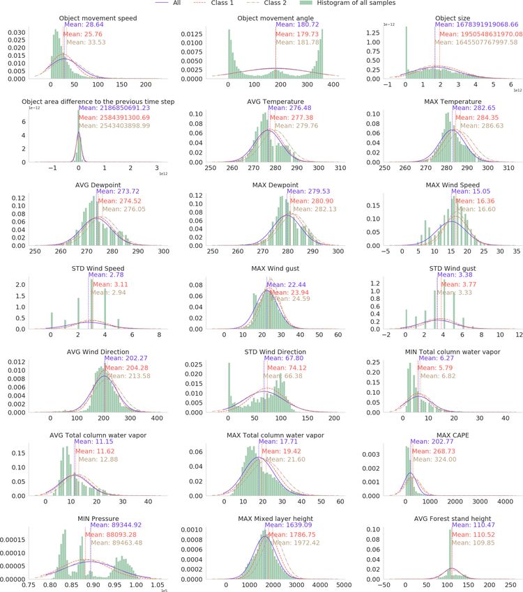
608                                                R. Tervo et al.: Predicting power outages caused by extratropical storms

report states that extratropical storm tracks are shifting to-     manner, connecting these fields (i.e., the natural hazard with
wards the poles, which might affect the storminess in north-       the societal factors) is done with machine learning (Chen
ern Europe. Thus, it may be concluded that the losses re-          et al., 2008).
lated to extratropical storms are also likely to increase, espe-      We present a novel method to identify, track, and classify
cially in northern Europe. However, as Barredo (2010) em-          extratropical storm objects based on how many power out-
phasizes, the cause for increased losses can at least partly be    ages they are expected to induce. We adapt convective storm
explained by the increasing exposure of society rather than        object detection (Rossi, 2015; Tervo et al., 2019; Cintineo
the increased number of windstorms.                                et al., 2014) to find potentially harmful areas from extrat-
   Several previous studies respond to the demand for storm        ropical storms by contouring objects from pressure and wind
impact estimation for power distribution, many of them fo-         gust fields. Instead of highly localized convective storms, we
cusing on the hurricane-induced power blackouts in northern        aim at larger but still regional geospatial accuracy so that, for
America (Eskandarpour and Khodaei, 2017; Guikema et al.,           example, damage in western and eastern Finland can be dis-
2014, 2010; Nateghi et al., 2014; Han et al., 2009; Wang           tinguished. We train a supervised machine-learning model to
et al., 2017; Allen et al., 2014; Chen and Kezunovic, 2016;        classify storm objects according to their damage potential. To
He et al., 2017; Liu et al., 2018). Convective thunderstorms       our knowledge, our method is the first that employs the extra-
have also been investigated thoroughly. Li et al. (2015) intro-    tropical storm objects as polygons and combines them with
duced an area-based outage prediction method further devel-        meteorological and non-meteorological features to predict
oped to take power grid topology into account (Singhee and         power outages. The method can be used as a decision sup-
Wang, 2017). Shield (2018) studied outage prediction by ap-        port tool in power distribution companies or as part of elabo-
plying a random forest classifier to weather forecast data in a    rating impact forecast by duty forecasters in national hydro-
regular grid. Kankanala et al. used data from ground observa-      meteorological centers. The ERA5 atmospheric reanalysis
tion stations and experimented regression (Kankanala et al.,       (Hersbach et al., 2018) provides the primary meteorological
2011), a multilayer perceptron neural network (Kankanala           input data for this study, while the national forest inventory
et al., 2012), and ensemble learning (Kankanala et al., 2014)      provided by The Natural Resources Institute Finland (Luke)
to predict outages caused by wind and thunder. The Bayesian        is used to represent the forest conditions in the prediction.
outage probability (BOP) prediction model developed by Yue         Finally, historical power outages from two sources are used
et al. (2018) combines weather radar data and unifies it to a      to train the model. However, the operational use of the model
regular grid. Cintineo et al. (2014) create spatial objects from   would require the use of weather prediction data instead of
satellite and weather radar data, and they track and classify      reanalysis.
the objects with the naïve Bayesian classifier. Rossi (2015)          This paper is organized as follows: Sect. 2 presents the
developed a method to detect and track convective storms.          used data, which is followed by a step-by-step method de-
The method was further developed to predict power outages          scription in Sect. 3. Section 3.1 discusses identifying storm
(Tervo et al., 2019).                                              objects and explains the storm tracking algorithm. Sec-
   While much work exists on damage caused by hurricanes           tion 3.2 considers storm and forest characteristics, hereafter
and convective thunderstorms, relatively few examples ex-          called features. Section 3.3 discusses how to define labels of
ist relating to outages caused by mid-latitude extratropical       storm objects based on the outage data. Section 3.4 describes
storms differing from hurricanes and convective storms in          the used machine-learning methods. In Sect. 4, we discuss
available data, time span, and applicable methods for detect-      the performance of the method. Finally, Sect. 5 includes a
ing and tracking. Extratropical storms are considered, for ex-     discussion and conclusions.
ample, in Yang et al. (2020), where different decision tree
methods are applied to a regular grid in the outage prediction
task. Cerrai et al. (2019) also use decision trees and regu-       2   Data
lar grids for the outage prediction, taking tree-leaf conditions
                                                                   We base our method on three main data sources: ERA5 re-
into account as a predictive feature. Related forest damage
                                                                   analysis data (Hersbach et al., 2019), a multi-source national
studies have been conducted with random forest classifiers
                                                                   forest inventory (ms-nfi) provided by the Natural Resources
and neural networks. Hart et al. (2019) showed that random
                                                                   Institute Finland (Luke), and occurred power outages ob-
forest regression and artificial neural networks could predict
                                                                   tained from two sources. First, the local dataset is gathered
the number of falling trees in France caused by the wind.
                                                                   from two power distribution companies, Loiste and Järvi-
Hanewinkel (2005) conducted a similar study in Germany
                                                                   Suomen Energia (JSE), located in eastern Finland. Second,
using artificial neural networks. Artificial neural networks
                                                                   the national dataset is obtained from Finnish Energy (ET), a
have been used to predict extreme weather in Finland (Ukko-
                                                                   branch organization for the industrial and labor market pol-
nen et al., 2017; Ukkonen and Mäkelä, 2019). The frame-
                                                                   icy of the energy sector. All data consider years from 2010
work of Masson-Delmotte et al. (2018) emphasizes that the
                                                                   to 2018.
impacts of extreme weather risks can be analyzed by estimat-
ing the hazard, vulnerability, and exposure. In an increasing

Nat. Hazards Earth Syst. Sci., 21, 607–627, 2021                                    https://doi.org/10.5194/nhess-21-607-2021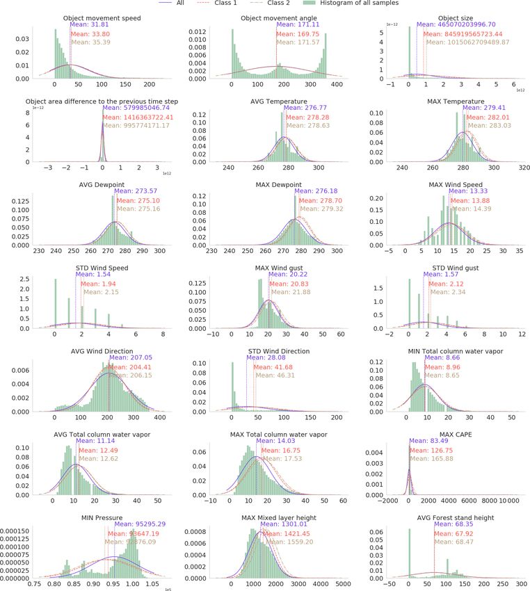
R. Tervo et al.: Predicting power outages caused by extratropical storms 609
ERA5 is the newest-generation reanalysis data provided
by ECMWF. ERA5 covers the years from 1979 onward
with a 1 h temporal resolution, has a horizontal resolution
of 31 km, and covers the atmosphere using 137 levels up to a
height of 80 km (Hersbach et al., 2019). Compared to in situ
wind observations, reanalysis data provide a spatiotempo-
rally wider dataset. However, a question may arise about the
accuracy of the reanalysis data. Ramon et al. (2019) exam-
ined the wind speed characteristics of a total of five state-of-
the-art global reanalyses concerning 77 instrumented towers.
In their study, ERA5 had the best agreement with in situ ob-
servations on daily timescales; this suggests the ERA5 wind
parameters to be adequate in windstorm damage examina-
tions as well. ERA5 data are also known to contain unrealisti-
cally large surface wind speeds in some locations (European
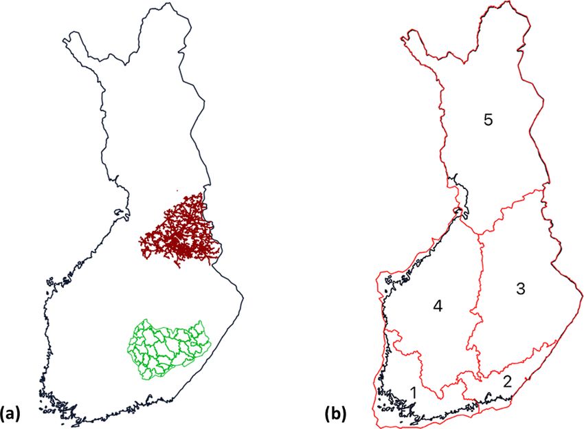
Centre for Medium-Range Weather Forecasts, 2019). None Figure 1. (a) Geographical coverage of the outage data (local
of these locations are, nevertheless, inside the geographical dataset). The red lines represent the power grid of Loiste (north-
domain of this work. ern grid company) and the green lines the operative areas of JSE
The multi-source forest inventory data are based on field (southern grid company). Outages of the local dataset are collected
measurements, satellite observations, digital maps, and other from both areas. (b) Regions in the national outage dataset. Out-
geo-referenced data sources (Mäkisara et al., 2016). The ages are gathered from all of Finland and aggregated to the regions
data consist of estimates for the forest age, tree species shown in the figure.
dominance, mean and total volume, and biomass (total
and tree-species-specific). The original geospatial resolution
of the data is 16 m, which has been reduced to approxi- described in more detail in Sect. 3.4, with both datasets to
mately 1.6 km resolution to speed up the processing. Tak- evaluate their performance for different types of data.
ing into account the size of extratropical cyclones (diameter
∼ 1000 km) and the wide areas where wind damage typically
3 Method
occurs near the cold front, we consider a resolution of 1.6 km
to be sufficiently high for modeling windstorm damage. We predict power outages by classifying storm objects iden-
Power outage data are obtained from two complementary tified from gridded weather data into three classes based on
sources. The national dataset is acquired from Finnish En- the number of power outages the storm typically causes. The
ergy (2010–2018), who aggregates the data from power dis- overall process consists of the following steps: (1) identify-
tribution companies in Finland. The national data are pro- ing storm objects from weather fields by finding contour lines
vided only for research purposes and for areas containing a of particular thresholds, (2) tracking the storm object move-
minimum of six grid companies; this is, for example, to en- ment, (3) gathering features of the storm objects, and (4) clas-
sure energy users’ anonymity. Therefore, the national dataset sifying each storm object individually. The classification is
does not include exact locations of the faults. We have also conducted for each storm object separately to distinguish the
obtained some parts of the data with better spatial accuracy different damage potential. Tracking is, however, necessary
from two individual power distribution companies. In this pa- to gather necessary features such as object movement speed
per, we refer to these data as the local dataset. In the local and direction. In the following, we discuss these phases in
dataset, the fault locations are reported in relation to trans- more detail.
formers; i.e., the spatial resolution of the outages ranges from
a few meters to kilometers. 3.1 Identifying and tracking storm objects
Figure 1 illustrates the geographical coverage of the
power outage data. The local dataset contains all outages Storm objects are identified by finding contour lines of 10 m
from 2010 to 2018 in the northern area (Loiste) and outages wind gust fields using 15 m s−1 thresholds from the ERA5
related to major storms in the southern area (JSE), shown in surface level grid with a time step of 1 h. The contouring al-
Fig. 1a. The national dataset contains all outages in Finland gorithm is capable of finding interior rings of the polygons.
from 2010 to 2018 divided into five regions, shown in Fig. 1b. The used wind gust fields did not, however, contain such
The national dataset contains in total 6 140 434 outages with cases. Thus one storm object represents a solid area (poly-
relatively low geographical accuracy. On the other hand, the gon) where the hourly maximum wind gust exceeds 15 m s−1
local dataset represents a substantially smaller geographical during one particular hour. The threshold of 15 m s−1 is se-
area with a good geographical accuracy but contains only lected as different sources indicate Finland being vulnerable
22 028 outages in total. We train our classification models, for windstorms and rather moderate winds (from 15 m s−1 )
https://doi.org/10.5194/nhess-21-607-2021 Nat. Hazards Earth Syst. Sci., 21, 607–627, 2021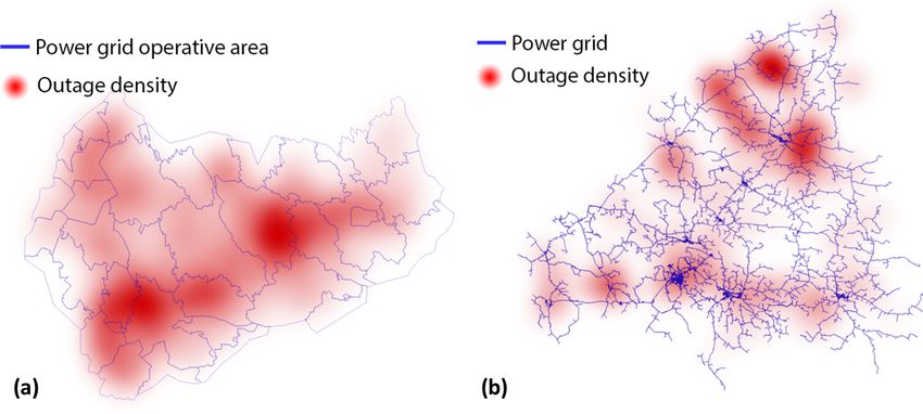
610 R. Tervo et al.: Predicting power outages caused by extratropical storms
causing damage to forests (Valta et al., 2019; Gardiner et al., in related studies (e.g., Suvanto et al., 2016; Peltola et al.,
2013). Valta et al. (2019) developed a method to estimate 1999; Valta et al., 2019) or identified through the empirical
the windstorm impacts on forests by combining the recorded experience of duty forecasters (Weather and Safety Center
forest damage from the nine most intense storms and their of Finnish Meteorological Institute – Duty forecasters, per-
observed maximum inland wind gusts. According to the sonal communication, May 2020). Second, we selected the
formula developed in the study, the inland wind gusts of relevant parameters, which were available to us or accessi-
15 m s−1 alone result in forest damage of 1800 m3 . We also ble with a reasonable effort. However, some possibly essen-
identify pressure objects by finding contour lines using a tial parameters, like soil temperature from ERA5 reanalysis,
1000 hPa threshold to connect potentially distant storm ob- were left out because of the slow downloading process.
jects around the low-pressure center to the same storm event. After the preliminary selection of the parameters, we con-
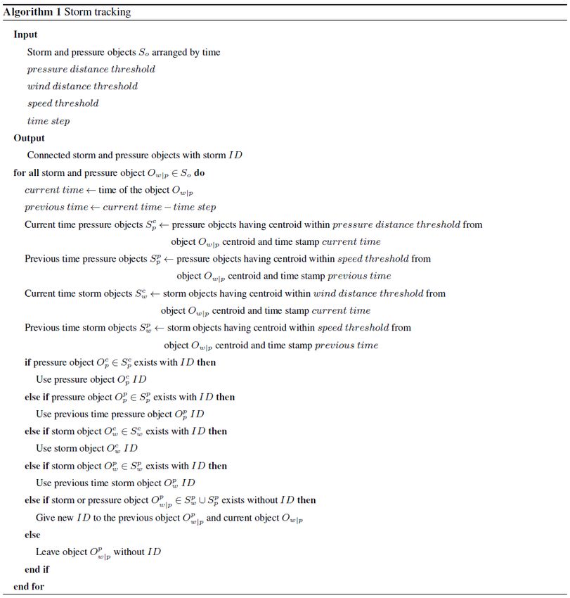
After identification, storm objects are tracked by connect- ducted dozens of light experiments using different combi-
ing them with each other. Each storm object is first connected nations of parameters and models to find the best possible
to nearby pressure objects from the current and preceding setup. To this end, we fitted the Gaussian distribution to each
time steps. If pressure objects do not exist within the dis- parameter using at first all samples, then samples with a few
tance threshold, the object is connected to nearby storm ob- outages, and finally samples with many outages (classes 1
jects from the current and preceding time steps. The algo- and 2 specified in Sect. 3.3). While many other distributions
rithm enables the assignment of each storm object to an over- are known to suit better in modeling particular parameters,
all event (low-pressure system) and tracking of the objects’ such as gamma in precipitation, Weibull in wind speed, and
movement. Algorithm 1 shows the details of the process. lognormal in cloud properties (Wilks, 2011), the Gaussian
We use a 500 km distance threshold for the distance be- distribution is a sufficient simplification to help in selecting
tween the storm and pressure objects. As the typical diame- relevant parameters. We visually inspected the differences
ter of an extratropical storm is approximately 1000 km (Gov- between fitted Gaussian distributions to deduce the poten-
orushko, 2011), we assume the damaging storm objects to tial relevance of the parameter. Supposedly the distribution
situate a maximum 500 km from the center of the low pres- of one parameter is different for all samples and samples with
sure. The threshold for movement speed is 200 km h−1 for many outages, and the classification method may exploit the
storm objects and 45 km h−1 for pressure objects. In other parameter to predict the damage potential of the storm object.
words, storm objects are not assumed to move more than The distributions of some selected parameters are shown in
200 km and pressure objects more than 45 km from the pre- Appendix A. In total, 35 parameters, shown as boldfaced in
ceding hourly time step (Govorushko, 2011). Convective Table 1, were chosen for the final classification.
storms may move faster but are outside the focus of this
work. 3.3 Defining classes
3.2 Extracting storm object features As shown in Fig. 2a and b, the outages in the local dataset
are concentrated heavily on “hot-spots”, probably due to for-
We characterize the storm objects identified by the methods est characteristics and network topology. The local dataset
discussed in Sect. 3.1 using the features listed in Table 1. contains 24 542 storm objects and 5837 outages connected
The features are structured as four groups. The first group to 2363 storm objects. Thus 22 179 storm objects in the
is a number of object characteristics such as size and move- local dataset did not cause any outages. The local power
ment speed and direction, which are calculated from the con- outage data contain 16 191 outages, which can not be con-
toured storm objects themselves. As the second group, rel- nected to any storm object. The national dataset contains
evant weather conditions, such as wind speed, temperature, 142 873 storm objects and 5 965 324 outages connected to
and others, are extracted from ERA5 data. We aggregate val- 33 796 storm objects. A total of 109 077 storm objects are
ues as a minimum, maximum, average, and standard devia- not connected to any outages, and 175 110 outages can not
tion calculated over all grid cells under the object coverage be connected to any storm object.
to represent each parameter with one number. Third, as most It should be noticed that the damage may occur anywhere
of the outages are caused by the trees falling on power grid in the power grid. Outages are, however, always reported
lines (Campbell and Lowry, 2012), the characteristics of the as transformers without electricity. Typically one instance
forest contribute to the damage (Peltola et al., 1999), and we of physical damage between the transformers causes several
complement our data with forest information. As for weather transformers to lose power. Power grid operators can often
parameters, values are aggregated over the storm object cov- turn part of the transformers back to operation even before
erage. The fourth group consists of the number of outages fixing the actual damage, which causes an unavoidable noise
and affected customers used as labels in the model training to the datasets.
process discussed in more detail in Sect. 3.4. Figure 3 represents the number of outages and storm ob-
We selected the 35 parameters based on two main crite- jects in both local and national datasets. We can identify a
ria. First, we prepared a list of potential parameters detected large number of 15 m s−1 storm objects in both sets, indicat-
Nat. Hazards Earth Syst. Sci., 21, 607–627, 2021 https://doi.org/10.5194/nhess-21-607-2021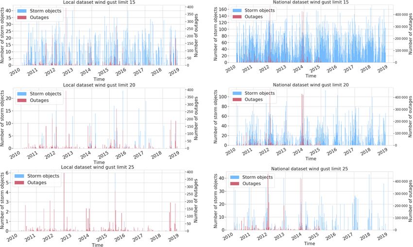
R. Tervo et al.: Predicting power outages caused by extratropical storms                                                    611

ing that moderate wind without other influencing factors does   Eino, Oskari, and Seija (Valta et al., 2019) hit Finland, both
not damage the transformers. When identifying storm objects     datasets contain plenty of storm objects with the 20 m s−1
with the contour of 20 and 25 m s−1 , the number of objects     threshold. Nevertheless, our experiments indicated that em-
decreases and starts to correlate more with a high number of    ploying 15 m s−1 storm objects yielded the best results. This
outages, which supports views of previous studies showing       is described more in Sect. 4.
the significance of stronger wind gusts to more severe storm       Figure 4 illustrates how many outages a single storm ob-
damage. The method seems to also identify the most critical     ject typically produces. In the local dataset, most of the storm
storm days by capturing several storm objects for those days.   objects cause only a few outages. Only 65 storm objects,
For instance, at the end of 2013, when the three major storms   which are only 0.3 % of the whole dataset, induced more than

https://doi.org/10.5194/nhess-21-607-2021                                Nat. Hazards Earth Syst. Sci., 21, 607–627, 2021
612                                                     R. Tervo et al.: Predicting power outages caused by extratropical storms

Table 1. Extracted features. Features used in the final classification are marked as bold.

  Feature                         Aggregation                                                Explanation
  Speed                           –                                                          Object movement speed
  Angle                           –                                                          Object movement angle
  Area                            –                                                          Object size
  Area difference                 –                                                          Object area difference to the previous time step
  Week                            –                                                          Week of the year
  Snow depth                      average, minimum, maximum                                  Snow depth
  Total column water vapor        average, minimum, maximum                                  Total amount of water vapor
  Temperature                     average, minimum, maximum                                  2 m air temperature
  Snowfall                        average, minimum, maximum, sum                             Snowfall (meter of water equivalent)
  Total cloud cover               average, minimum, maximum                                  Total cloud cover (0–1)
  CAPE                            average, minimum, maximum                                  Convective available potential energy (J kg−1 )
  Precipitation kg m−2            average, minimum, maximum, sum                             Precipitation amount (kg m−2 )
  Wind gust                       average, minimum, maximum, standard deviation              Hourly maximum wind gust (m s−1 )
  Wind speed                      average, minimum, maximum, standard deviation              10 m wind speed (m s−1 )
  Wind direction                  average, minimum, maximum, standard deviation              Wind direction (◦ )
  Dew point                       average, minimum, maximum                                  Dew point
  Mixed-layer height              average, minimum, maximum                                  Boundary layer height
  Pressure                        average, minimum, maximum                                  Air pressure
  Forest age                      average, minimum, maximum, standard deviation              The age of the growing stock on a forest stand
  Forest site fertility           average, minimum, maximum, standard deviation              Group of the forest by vegetation zones
  Forest stand mean diameter      average, minimum, maximum, standard deviation              Forest stand mean diameter
  Forest stand mean height        average, minimum, maximum, standard deviation              Forest stand mean height
  Forest canopy cover             average, minimum, maximum, standard deviation              Forest canopy cover fraction (0 %–100 %)
  Outages                         –                                                          Number of occurred outages
  Customers                       –                                                          Number of affected customers
  Transformers                    –                                                          Number of transformers under the object
  All customers                   –                                                          Number of customers under the object
  Class                           –                                                          Assigned class

Figure 2. Spatial distribution of the outages between 2010 and 2018 visualized as a spatial heat map. (a) JSE network (southern area) and
(b) Loiste network (northern area).

10 outages. On the other hand, in the national dataset where               figure contains all outages in both datasets, whether they
one storm object typically affects several different transform-            are related to a storm or not. In the local dataset, usually
ers, 17 587 storm objects have caused more than 10 outages,                20–30 customers lose electricity in one outage. In the na-
representing 12 % of the whole dataset. Figure 5 renders how               tional dataset, only six customers usually lose electricity in
many customers are typically affected by one outage. The                   one outage. We assume that this is due to different network

Nat. Hazards Earth Syst. Sci., 21, 607–627, 2021                                             https://doi.org/10.5194/nhess-21-607-2021
R. Tervo et al.: Predicting power outages caused by extratropical storms                                                               613

Figure 3. Storm object time series (15, 20, and 25 m s−1 contours) with occurred outages for local and national datasets.

topologies between the areas. Notably, in some rare cases, a            Table 2. Class definitions.
much higher number of customers are affected. We assume
that these cases typically occur in urban areas and are rare                Class    Outage      Local       Local    Outage    National
because the power network is mainly underground in these                             limit in   dataset    limit in   dataset
areas.                                                                                dataset      size   national       size
                                                                                                            dataset
   We use three classes designed together with power grid
companies aiming at a simple “at glance” view for power grid                0             0      5624           0     76 215
operators. Class 0 represents no damage, class 1 low damage,                1           1–3       353       1–140     14 417
and class 2 high damage. As the number of outages produced                  2           ≥4        181       ≥ 141      3085
by a single storm object varies significantly in the local and
national datasets, we decided to define separate limits for the
local and the national datasets. The detailed limits are listed         2002). SMOTE creates new training samples based on their
in Table 2. Class 1 is defined such that it represents roughly          k = 5 nearest neighbors following
80 % of all cases with at least one outage. Class sizes are
highly imbalanced as most of the storm objects do not cause             xnew = xi + λ × (xzi − xi ) ,                                      (1)
any damage.
                                                                        where xi is an original class sample, xzi is one of xi ’s k near-
                                                                        est neighbors, and λ is a random variable drawn uniformly
3.4   Classifying storm objects
                                                                        from the interval [0, 1]. After augmentation, all classes have
                                                                        an equal number of samples, which reduces the tendency of
We centered and normalized the data points by subtracting               classification methods to always predict the majority class.
the empirical mean and then dividing it by the empirical stan-             Five different models were evaluated to classify storm ob-
dard deviation. The hyperparameters were determined using               jects. We omit the mathematical definitions but shortly dis-
random-search five-fold cross-validation (Bergstra and Ben-             cuss the characteristics of different models and describe the
gio, 2012). To cope with the imbalanced class distribution,             implementation details chosen in this work.
we generate artificial training samples using the synthetic
minority over-sampling technique (SMOTE) (Chawla et al.,

https://doi.org/10.5194/nhess-21-607-2021                                           Nat. Hazards Earth Syst. Sci., 21, 607–627, 2021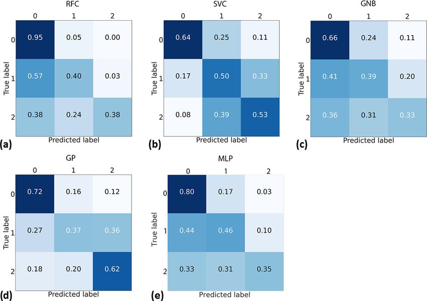
614                                                   R. Tervo et al.: Predicting power outages caused by extratropical storms

Figure 4. Number of storm objects per caused outage in the (a) local dataset and (b) national dataset.

Figure 5. Relationship between number of outages and affected customers in the (a) local dataset and (b) national dataset.

3.4.1   Random forest classification (RFC)                               Table 3. Hyperparameters for the RFC.

RFC is based on a random ensemble of decision trees and                          Parameter                          Value
aggregating results from individual trees to the final esti-                     Number of trees in the forest      500
mate. Trees in the ensemble are constructed with four steps:                     Max depth                          unlimited
(1) use bootstrapping to generate a random sample of the                         Minimum no. of samples to split    2
data, (2) randomly select a subset of features at each node,                     Minimum no. of samples to leaf     1√
(3) determine the best split at the node using loss function,                    Features to consider for split       num.of feat.
and (4) grow the full tree (Breiman, 2001). RFC is good to                       Max no. of leaf nodes              unlimited
cope with high-dimensional data. It has also been found to
provide adequate performance with imbalanced data (Tervo
et al., 2019; Brown and Mues, 2012) and is widely used
with weather data (e.g., Karthick et al., 2020; Cerrai et al.,           between training samples and the hyperplane. The hyper-
2019; Lagerquist et al., 2017). The method is prone to over-             planes may be constructed with nonlinear kernels such as
fit, which is why hyperparameter tuning is very important.               the Gaussian radial basis function (RBF) (Shawe-Taylor and
Hyperparameters used in this work are listed in Table 3. We              Cristianini, 2004) that often reform a nonlinear classification
use RFC with the Gini impurity loss function.                            problem to a linear one. Operating in the high-dimensional
                                                                         feature space without additional computational complexity
3.4.2   Support vector classifiers (SVCs)                                makes SVCs an attractive choice to extract meaningful fea-
                                                                         tures from a high-dimensional dataset. A domain-specific ex-
SVCs construct a hyperplane or classification function in                pert knowledge can also be capitalized on the kernel design.
a high-dimensional feature space and maximize a distance                 On the other hand, finding the correct kernel is often a dif-

Nat. Hazards Earth Syst. Sci., 21, 607–627, 2021                                           https://doi.org/10.5194/nhess-21-607-2021
R. Tervo et al.: Predicting power outages caused by extratropical storms 615
ficult task. Training SVCs is a convex optimization prob- 3.4.4 Gaussian processes (GPs)
lem, meaning that it has no local minima. Depending on the
kernel, a training process may, however, be a very memory- The GP (Rasmussen, 2003) is a non-parametric probabilis-
intensive process. tic method that interprets the observed data points as real-
Suppose the SVC output is assumed to be the log odds of a izations of a Gaussian random process. The GP is widely
positive sample. In that case, one can fit a parametric model used for example in weather observation interpolation krig-
to obtain the posterior probability function and thus get prob- ing (Holdaway, 1996). The GP is a very flexible and pow-
abilities for samples to belong to the particular class (Platt, erful but computationally expensive method, which tends to
1999). For more details, we request the reader to consult for lose its power with high-dimensional data. The GP hinges on
example Chang and Lin (2011) and Platt (1999). a kernel function that encodes the covariance between dif-
We implement the SVCs in two phases. First, we sepa- ferent data points. As a kernel, we use a product of a dot-
rate class 0 (no outages) and other samples employing SVCs product kernel (Eq. 3) and pairwise kernel with Laplacian
with the radial basis function (RBF), defined in Eq. (2). Sec- distance (Rupp, 2015), defined in Eq. (4). The kernel param-
ond, we distinguish classes 1 and 2 using SVCs with a dot- eters were optimized on the training data by maximizing the
product kernel defined in Eq. (3) (Williams and Rasmussen, log-marginal likelihood.
2006). The second phase is performed only for the samples kpairwise (x, x 0 ) = exp −γ kx − x 0 k1 ,
(4)
predicted to cause outages in the first phase. The approach is
similar to the often-used one-vs.-one classification, where a where x and x 0 are two samples in the input space and γ is a
binary classifier is fitted for each pair of classes. In our case kernel coefficient parameter.
different kernels were used for different pairs.
3.4.5 Multilayer perceptrons (MLPs)
2
kRBF (x, x 0 ) = exp −γ x − x 0 , (2)
MLPs (Goodfellow et al., 2016) are the most basic form
of artificial neural networks. With good results achieved by
where x and x 0 are two samples in the input space and γ is a MLPs in predicting storms (Ukkonen and Mäkelä, 2019),
kernel coefficient parameter. they are a natural choice for experimentation in this work.
Neural networks are very adaptive methods as they can learn
k· (x, x 0 ) = σ0 + x · x 0 , (3)
a representation of the input at their hidden layers. Unlike
where x and x 0 are two samples in the input space and σ is a GNBs, they do not make any assumptions about the distribu-
kernel inhomogeneity parameter. tion of the data. As a downside, MLPs require large amounts
of data, and the training process is computing-intensive. They
3.4.3 Gaussian naïve Bayes (GNB) also have a large number of hyperparameters to be optimized,
including the correct network topology.
GNB (Chan et al., 1982) is a well-known and widely We searched the correct model parameters and network
used method based on the Bayesian probability theory. The topology for local and national datasets by running multiple
method assumes that all samples are independent and identi- iterations of random-search five-fold cross-validation to ob-
cally distributed (i.i.d.), which does not naturally hold for the tain the best possible micro-average of the F1 score (defined
weather data. Despite the internal structure of the data, GNB in Sect. 4) employing the Talos library (Autonomio, 2020).
is still used for weather data (e.g., Kossin and Sitkowski, The final setup is composed of a Nadam optimizer (Dozat,
2009; Cintineo et al., 2014; Karthick et al., 2020) and worth 2016), random normal initializer, and ReLU activation func-
investigating in this context. The classification rule in GNB is tion for hidden layers. Binary cross-entropy was used as a
n
Q
ŷ = argmaxy P (y) P (xi |y), where P (y) is a frequency of loss function. Optimal network topology varied in different
i=1 datasets: for the local dataset, the best results were obtained
class y and P (xi |y) is a likelihood of the ith feature assumed with a network containing three hidden layers with 75, 145,
to be Gaussian. Because of the naïve i.i.d. assumption, each and 35 neurons. For the national dataset, the best results
likelihood can be estimated separately, which helps to cope were obtained with a network containing three hidden lay-
with a curse of dimensionality and enable GNB to work rela- ers with 75, 195, and 300 neurons. During the optimization
tively well with small datasets. On the other hand, estimating process, the results varied between different setups from 0.6
likelihoods can be done effectively and iteratively, enabling to 0.95 in terms of the F1 score.
the GNB to scale to large datasets. As a downside, the sim-
ple method may lack expression power to perform well in a
complex context. 4 Results
We used two different methods for splitting the data into
training and test sets. The first method is uses 25 % of ran-
domly picked samples in the test set. The second method
https://doi.org/10.5194/nhess-21-607-2021 Nat. Hazards Earth Syst. Sci., 21, 607–627, 2021616 R. Tervo et al.: Predicting power outages caused by extratropical storms
is to construct a test set from a 1-year continuous time Tables 4 and 5 divulge the results for each model using
range (2010–2011). Both approaches have their advantages. the local and national datasets, respectively. Models trained
A continuous time range ensures that the model has not seen with the local dataset can reach the better-weighted F1 score,
any autocorrelated samples caused by an internal structure while the best models trained with the national dataset pro-
of the weather data in the training phase (Roberts et al., vide a significantly better macro-average of the F1 score. The
2017). However, having only 9 years of data from a relatively national dataset contains many more samples in classes 1
small geographical area, the continuous test set cannot con- and 2, which enables models to learn the classes better and
tain many storms as most of the data need to be reserved for thus enhance the macro-average of the F1 score. Whether
the training process. Thus, the test set may only contain a sin- the test set is randomly chosen or continuous does not seem
gle type of storm for which the model may work especially to make a large difference in most cases. The only affected
well or bad. Picking the test set randomly minimizes this risk model is the RFC, having contradictory better results trained
and provides more insight into the model performance. with the continuous test set from the local dataset and the
We evaluate the models with a weighted average of pre- random test set from the national dataset. This reveals more
cision and recall and both weighted and macro-averages of about the unstable performance of RFC than the relevance of
the F1 score. Precision (Eq. 5) reports how many samples the dataset split method.
are correctly predicted to belong to a class. Recall (Eq. 6) The confusion matrices are depicted in Fig. 6. RFC pro-
tells how many samples belonging to a class are found in vides the best results in terms of the selected metrics. How-
the prediction. The F1 score (Eqs. 7 and 8) calculates a har- ever, closer exploration reveals that this performance is
monic mean of precision and recall. Finally, as the datasets largely due to the best performance in predicting class 0,
are extremely imbalanced, we calculate a weighted average which is the largest class. SVC results are some of the most
of the metrics utilizing a number of samples in each class balanced ones, being the best only in the local dataset with a
and a macro-average of the F1 score using an average of the random test set but yielding good stable results in all cases.
F1 score of each class. A model with a higher macro-average The confusion matrix, shown in Fig. 6b, displays that it is
of the F1 score performs better with small classes. The se- not the best model to predict class 0, but only a small share
lected metrics do not take a distance between predicted and of true class 2 cases and the smallest share of true class 1
true class into account. It is naturally worse to predict, for cases are predicted as class 0. That is to say, SVCs miss the
example, class 0 (no damage) in the case of a true class 2 smallest number of destructive storms, although it confuses
(high damage) than in the case of a true class 1 (low dam- the amount of caused damage.
age). We decided, however, to use metrics that measure the The GP is another strong option that performs even bet-
method performance properly with imbalanced classes. ter with class 0 while still providing good performance with
class 2. A significant connecting aspect between the GP and
1 X tp SVCs is an almost identical kernel. Based on these exper-
Precision = P |ŷc | , (5)
|ŷc | cı C tp + fp iments, RBF and pairwise kernels separate harmless and
c∈C harmful samples from each other while the dot-product ker-
where C represents the set of classes, ŷ predicted the class, nel separates classes 1 and 2 even better than exponential
“tp” is true positives, and “fp” is false positives. functions. We select the GP for further analysis in this paper
since it provides the best performance in class 2.
Using the 15 m s−1 threshold for detecting storm objects
1 X tp
Recall = P |ŷc | , (6) yields clearly better results than the 20 m s−1 threshold. For
|ŷc | c∈C tp + fn
c∈C example, SVCs trained with the national dataset using the
20 m s−1 threshold and randomly chosen test set provide only
where C represents the set of classes, ŷ predicted the class, a 0.48 macro-average of the F1 score, 12 percentage points
“tp” is true positives, and “fn” is false negatives. below the corresponding model using the 15 m s−1 thresh-
old. The 15 m s−1 threshold has two major advantages com-
1 X precisionc × recallc
F1weighted = P |ŷc | , (7) pared to the 20 m s−1 threshold. First, it provides a signifi-
|ŷc | c∈C precisionc + recallc cantly larger dataset, and second, in contrast to the 20 m s−1
c∈C
threshold, it is able to catch virtually all extratropical storms
where C represents the set of classes, ŷ predicted the class, that cause outages.
precision is defined in Eq. (5), and recall is defined in Eq. (6).
4.1 Feature importance in the model performance
1 X precisionc × recallc
F1macro = , (8)
|C| c∈C precisionc + recallc The relevance of the individual predictive features can be ex-
plored by using the permutation test, as done by Breiman
where C represents the set of classes, precision is defined in (2001). First, the baseline score of the fitted model is calcu-
Eq. (5), and recall is defined in Eq. (6). lated using the test set. Then each feature is randomly per-
Nat. Hazards Earth Syst. Sci., 21, 607–627, 2021 https://doi.org/10.5194/nhess-21-607-2021R. Tervo et al.: Predicting power outages caused by extratropical storms 617
Table 4. Results for each model trained with the local dataset obtained from two local power grid companies (defined in Sect. 3.3). The results
with boldfaced font represent the best achieved results within the metric, shown separately for the random and continuous split methods.
Model Split method Precision Recall Weighted F1 score Macro-average F1 score
Test Test Train Test Train Test
Random forest classifier (RFC) Random 0.82 0.76 0.93 0.79 0.93 0.40
Continuous 0.88 0.91 0.93 0.89 0.93 0.48
Support vector classifier (SVC) Random 0.85 0.73 0.78 0.78 0.78 0.44
Continuous 0.87 0.72 0.77 0.78 0.77 0.42
Gaussian naïve Bayes (GNB) Random 0.87 0.61 0.59 0.70 0.59 0.42
Continuous 0.89 0.59 0.59 0.69 0.59 0.40
Gaussian process (GP) Random 0.84 0.70 1.0 0.76 1.0 0.43
Continuous 0.85 0.67 0.94 0.74 0.94 0.41
Multilayer perceptron (MLP) Random 0.82 0.81 0.98 0.80 0.91 0.41
Continuous 0.81 0.79 0.97 0.80 0.91 0.41
Table 5. Results for each model trained with the national dataset covering all of Finland (defined in Sect. 3.3). The results with boldfaced
font represent the best achieved results within the metric, shown separately for the random and continuous split methods.
Model Test set split Precision Recall Weighted F1 score Macro-average F1 score
Method Test Test Train Test Train Test
Random forest classifier (RFC) Random 0.83 0.84 1.0 0.83 1.0 0.62
Continuous 0.77 0.81 1.0 0.78 1.0 0.40
Support vector classifier (SVC) Random 0.81 0.61 0.68 0.68 0.68 0.60
Continuous 0.62 0.60 0.60 0.60 0.60 0.60
Gaussian naïve Bayes (GNB) Random 0.75 0.60 0.66 0.66 0.45 0.39
Continuous 0.77 0.60 0.45 0.66 0.45 0.40
Gaussian process (GP) Random 0.57 0.56 0.71 0.55 0.71 0.55
Continuous 0.67 0.65 0.94 0.65 0.94 0.61
Multilayer perceptron (MLP) Random 0.79 0.75 0.94 0.77 0.90 0.52
Continuous 0.76 0.78 0.93 0.78 0.85 0.40
muted, and the difference in the scoring function is calcu- tive of all meteorological parameters used in the training. In
lated. The random permutation is repeated 30 times for each other words, all employed meteorological parameters are im-
parameter, and the average of the results is used. The pro- portant for the prediction, while different aggregations con-
cedure offers information on how important the feature is to tribute to the “fine-tuning” of the model.
obtain good results. It should be mentioned that highly corre- As Fig. 7 shows, the most significant parameter regarding
lated features may get low importance as other features work our model performance is the average wind speed. Numerous
as a proxy to the permuted feature. However, using com- studies support our result of wind being the most important
pletely independent features is not possible in weather data damaging factor (Virot et al., 2016; Valta et al., 2019; Jokinen
since weather parameters are often dependent on each other, et al., 2015). However, the studies highlight the importance
and eliminating even the most apparent pairs from the used of maximum wind gusts instead of the average wind. Surpris-
features impaired the results in our experiments. ingly, in our analysis, the wind gust speed does not belong to
We used the macro-average of F1 defined in Eq. (8) as the most critical parameters. Instead, maximum mixed-layer
a scoring function and the randomly selected test set from height, related to the wind gustiness, contributes crucially to
the national data. The relevance is shown in Fig. 7. Most the model performance. The dependencies between predic-
features show at least a little relevance for the results. The tive features might be one reason for some parameters to have
first 12 features are significantly more relevant than the rest. a lower rank in the results.
The most important features contain at least one representa-
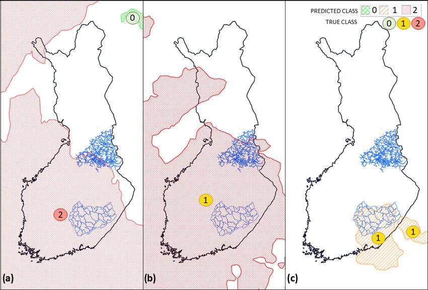
https://doi.org/10.5194/nhess-21-607-2021 Nat. Hazards Earth Syst. Sci., 21, 607–627, 2021618 R. Tervo et al.: Predicting power outages caused by extratropical storms Figure 6. Confusion matrices produced using the randomly selected national dataset and (a) RFC, (b) SVC, (c) GNB, (d) GP and (e) MLP. Each cell of the confusion matrices represents a share of predictions having a corresponding combination of predicted and true class. For example, the middle right cell tells the share of samples belonging to class 1 but predicted to have class 2. Figure 7. Permutation feature importance using the GP classification method trained with the randomly selected national dataset. The higher the effect on the F1 score (y axis), the bigger the significance. The stand mean diameter and height are the most impor- age. However, in the feature importance test, forest age does tant features regarding the forest parameters, which corre- not seem to contribute significantly to the prediction out- sponds to our expectations. Previous studies also show these come. features influence the wind damage in forests (Pellikka and The most important object feature is the size of the ob- Järvenpää, 2003) and hence indirectly electricity grids. As ject. Object movement speed and direction did not contribute Pellikka and Järvenpää (2003) and Suvanto et al. (2016) dis- strongly to the results. However, previous studies indicate cuss, the age of the forest also has an impact on storm dam- that besides the size of the impacted area, the duration of Nat. Hazards Earth Syst. Sci., 21, 607–627, 2021 https://doi.org/10.5194/nhess-21-607-2021
R. Tervo et al.: Predicting power outages caused by extratropical storms                                                     619

strong winds – i.e., the propagation speed of the system – also   of Finland for various reasons. The trees still carried leaves,
influences the amount of damage (Lamb and Knud, 1991).            the soil was wet after a rainy August, the strong wind areas
                                                                  of Rauli were widespread, and the solar radiation intensified
4.2     Case examples                                             the wind gusts during the afternoon (Finnish Meteorologi-
                                                                  cal Institute, 2016). Rauli impacted the middle and southern
We illustrate the prediction produced using the GP classifica-    parts of Finland in particular, which are also the most densely
tion method with the three most interesting examples of well-     populated areas. The power outages increased rapidly in the
known storms in Fig. 8. We chose the cases among a number         middle part of Finland, starting at midday and reaching the
of test cases to illustrate the strengths and weaknesses of the   highest values, 200 000 households without electricity (Ilta-
method. The examples are chosen from the randomly picked          Sanomat, 2016), around 17:00 UTC. The winds blew excep-
test set, which was not used to train the model. Because of       tionally long, nearly 24 h. The typical duration of summer
the random sample, we cannot represent the entire prediction      storms is between 6–12 h.
of individual storms, only individually picked time steps. In        Figure 8b shows the predicted outages and true classes
two of the example cases, the model performs well (storms         at 12:00 UTC, 27 August 2016. In this particular time step,
Tapani and Pauliina) and in one case (storm Rauli) less accu-     the model overpredicts the class; however, the predicted out-
rately.                                                           age area seems to correlate with the wind gust maxima of
                                                                  that afternoon. The strongest wind gusts were measured in
4.2.1    Event 1: extratropical storm Tapani
                                                                  the southern and middle parts of the country, with maximum
         (26 December 2011)
                                                                  gusts reaching up to 24.9 m s−1 at land stations (Klemettilä,
The first example is one of the most known extratropi-            Vaasa and Maaninka, Pohjois-Savo) and in wide areas up to
cal storms in Finland. Storm Tapani, also known as Cy-            20 m s−1 apart from the northern part of Finland.
clone Dagmar (Kufeoglu and Lehtonen, 2015), was a rare
winter storm, causing broad and long-lasting electricity in-      4.2.3   Event 3: extratropical storm Pauliina
terruptions. Extreme wind gusts of over 30 m s−1 caused                   (22 June 2018)
widespread damage, especially in the southern and west-
                                                                  The last example is a strong extratropical storm, called Pauli-
ern parts of the country. Approximately 570 000 households
                                                                  ina (Finnish Meteorological Institute, 2018), that caused nu-
were left without electricity, causing EUR 30 million of re-
                                                                  merous power outages in Finland. The most significant part
pair costs and EUR 80 million of monetary compensation for
                                                                  of the power outages happened in the network of the power
electricity distribution companies to their customers (Han-
                                                                  grid company JSE included in the local dataset. The high-
ninen and Naukkarinen, 2012). An exceptionally warm De-
                                                                  est peak in the damage was reached between 18:00 and
cember and the warmest Boxing Day in 50 years (Finnish
                                                                  20:00 UTC with over 28 000 households without electric-
Meteorological Institute, 2011) resulted in wet and unfrozen
                                                                  ity. The strongest wind gust on land reached 22.7 m s−1 in
soil. Thus, the trees were poorly anchored and exposed to
                                                                  Helsinki, Kumpula observation station, and the inland gusts
significant storm damage.
                                                                  were widely between 15–20 m s−1 (Finnish Meteorological
   Figure 8a represents the outage prediction (raster-covered
                                                                  Institute, 2020; Finnish Meteorological Institute – Twitter,
areas) and the actual true classes (numbers) based on the
                                                                  2020). The strong wind gusts continued until the dawn of
damage data at 15:00 UTC, 26 December 2011. Wide areas
                                                                  23 June.
in central and western parts of Finland are predicted to have
                                                                     Figure 8c presents the predicted and true damage classes
high (class 2) damage. The predicted class is in line with
                                                                  at 01:00 UTC, 22 June 2018. We chose extratropical storm
the true class. Also, the damage areas of the storm corre-
                                                                  Pauliina as an example storm for two reasons: (1) Pauliina
late with the wind gust observations of the Finnish Meteo-
                                                                  represents a low-damage class and (2) Pauliina represents a
rological Institute. The strongest gusts occurred in western
                                                                  rare, summer-season extratropical storm. Figure 8c shows the
(15–27 m s−1 ) and southern (18–28 m s−1 ) Finland and the
                                                                  predicted and true classes correlating. While weather warn-
northwestern part of Lapland (13–31 m s−1 ) (Finnish Mete-
                                                                  ings were issued to large areas in the southern and middle
orological Institute, 2020). In the rest of Finland, the maxi-
                                                                  parts of Finland, myrskyvaroitus.com (2018) predicted and
mum wind gusts remained between 10–15 m s−1 , and there-
                                                                  true damage to the power grid occurred in a relatively small
fore the damage were minor. Overall, the model predicted the
                                                                  geographical area.
damage accurately in this particular example.

4.2.2    Event 2: extratropical storm Rauli
         (27 August 2016)                                         5   Discussion and conclusions

Extratropical storm Rauli was an exceptionally strong sum-        This paper introduces a novel method to predict the damage
mer storm, especially regarding the impacts. It caused severe     potential of extratropical storms to power grids. The method
damage to the power grid in the western and middle parts          consists of identifying storm objects by contouring surface

https://doi.org/10.5194/nhess-21-607-2021                                  Nat. Hazards Earth Syst. Sci., 21, 607–627, 2021
620 R. Tervo et al.: Predicting power outages caused by extratropical storms Figure 8. Selected examples. (a) Extratropical storm Tapani (26 December 2011 11:00 UTC), (b) extratropical storm Rauli (27 August 2016 10:00 UTC), and (c) extratropical storm Pauliina (22 June 2018 01:00 UTC), produced by employing the SVC model trained with the national dataset. The storm objects are colored based on the predicted class while the true class is stated as a colored number over the object. wind gust fields with the 15 m s−1 threshold along with pres- and movement. Moreover, objects are easy to visualize, and sure objects with a 1000 hPa threshold, tracking the objects, user interfaces may be enriched with related actions such as and then classifying them into three classes based on their tracking and alarms. damage potential to the power grid. For the classification On the other hand, storm objects use only aggregated task, we evaluated five different machine-learning methods, attributes, which may decrease the classification accuracy all employing a total of 35 predictive features and trained when predictive features vary significantly under the storm with 8 years of power outage data from Finland. object area. Several machine-learning methods, i.e., deep Both Gaussian processes and support vector classifiers neural networks, could be trained to employ those local fea- provided good results. The model recognizes harmful storm tures to gain better accuracy. Such methods could also utilize objects well and can distinguish extremely harmful objects three-dimensional data. among others adequately. While the results still leave a lot to The fixed thresholds of wind gust and pressure were used improve, the developed model can already be used to support to extract the storm objects in this paper. Although the previ- decisions in power grid companies. In some cases, the model ous studies indicate the critical threshold of wind gust speed is able to provide a more specific and geospatially accurate to be the same for almost the entire geospatial domain of this prediction of potential damage to the power grid than, for ex- work (Gardiner et al., 2013), it would be beneficial to adapt ample, weather warning. The evaluation was, however, based the threshold based on the geographic location using, for ex- on the ERA5 reanalysis data. Using the method in an oper- ample, the storm severity index (SSI) originally introduced ational setting would require weather prediction data, which in Leckebusch et al. (2008). Moreover, the correct threshold introduces additional uncertainty to the outage prediction. may vary depending on the data source. The presented object-based approach has both advantages The work opens several possible avenues for further stud- and disadvantages. Extracting storm objects in advance pre- ies. It would be interesting to compare the current solution processes the data for machine-learning techniques, such with a grid-based approach and deep neural networks. In- as RFC, which do not perform feature learning. It enables cluding data on soil moisture, soil temperature, and leaf in- machine-learning methods to focus only on the relevant parts dex would most likely enhance the results, if available with of the data. Methods not containing feature learning, such as sufficient spatial and temporal resolution, since they would RFC and logistic regression, have been found to outperform provide critical information about the environmental condi- neural networks for forest (Hart et al., 2019) and weather data tions. Different thresholds could be investigated as well, es- (Tervo et al., 2019). It also leads to significantly faster train- pecially for pressure objects where lower thresholds might ing times. Processing objects instead of the grid also makes yield better results. By design, applying the method to other it easier to track and use object attributes such as age, speed, regions is possible, but it is subject to the availability of Nat. Hazards Earth Syst. Sci., 21, 607–627, 2021 https://doi.org/10.5194/nhess-21-607-2021
R. Tervo et al.: Predicting power outages caused by extratropical storms                                                    621

power outage records, forest inventory, impact, and meteo-           Experiments in this study were conducted with ERA5 re-
rological data. For the classification task, carefully designed   analysis and additional forest data. As the method employs
Bayesian networks could provide good results as well. Es-         common features also existing in various other datasets, data
pecially in the randomly selected test set, data may be au-       provided by other vendors could be used as well. By employ-
tocorrelated, which may lead to unrealistically good results.     ing weather forecasts as input, this method could be used
We have addressed this issue by also using a continuous time      as a base for a decision support tool and as part of an ex-
series (from 2010 to 2011) for the test set. The evaluation       isting early warning system for both duty forecasters of na-
could also be extended with a leave-one-day-out or leave-         tional hydro-meteorological centers and operators of electric-
one-week-out method where for each week 1 d or for each           ity transmission companies.
month 1 week is left out for validation purposes.
   End users, especially expert users like duty forecasters,
might benefit from the uncertainty information originating as
the probabilistic prediction of the classification model. How-
ever, the presentation of such information should be very
carefully chosen to not mislead non-expert users for over-
confidence.

https://doi.org/10.5194/nhess-21-607-2021                                  Nat. Hazards Earth Syst. Sci., 21, 607–627, 2021
You can also read