Practical Machine Learning - A New Look at Anomaly Detection - Ted Dunning & Ellen Friedman
←
→
Page content transcription
If your browser does not render page correctly, please read the page content below

Practical Machine
Learning
A New Look at Anomaly Detection

Ted Dunning &
Ellen Friedman
®   Sandbox
    Fast
    The first drag-and-drop
    sandbox for Hadoop
    Free
    Fully-functional virtual
    machine for Hadoop
    Easy
    Point-and-click tutorials
    walk you through
    the Hadoop experience

    www.mapr.com/sandboxML

    Use the Sandbox to tackle
    anomaly detection
    as described in the book!
Practical Machine Learning
  A New Look at Anomaly Detection

      Ted Dunning and Ellen Friedman
Practical Machine Learning
by Ted Dunning and Ellen Friedman
Copyright © 2014 Ellen Friedman and Ted Dunning. All rights reserved.
Printed in the United States of America.
Published by O’Reilly Media, Inc., 1005 Gravenstein Highway North, Sebastopol, CA
95472.
O’Reilly books may be purchased for educational, business, or sales promotional use.
Online editions are also available for most titles (http://my.safaribooksonline.com). For
more information, contact our corporate/institutional sales department: 800-998-9938
or corporate@oreilly.com.
Editor: Mike Loukides

June 2014:                First Edition

Revision History for the First Edition:
2014-05-14:      First release

See http://oreilly.com/catalog/errata.csp?isbn=9781491904084 for release details.

Nutshell Handbook, the Nutshell Handbook logo, and the O’Reilly logo are registered
trademarks of O’Reilly Media, Inc. Practical Machine Learning: A New Look at Anom‐
aly Detection and related trade dress are trademarks of O’Reilly Media, Inc.
Many of the designations used by manufacturers and sellers to distinguish their prod‐
ucts are claimed as trademarks. Where those designations appear in this book, and
O’Reilly Media, Inc. was aware of a trademark claim, the designations have been printed
in caps or initial caps.
Photos are copyright Ellen Friedman.
While every precaution has been taken in the preparation of this book, the publisher
and authors assume no responsibility for errors or omissions, or for damages resulting
from the use of the information contained herein.

ISBN: 978-1-491-90408-4
[LSI]

Table of Contents

1. Looking Toward the Future. . . . . . . . . . . . . . . . . . . . . . . . . . . . . . . . . . . . 1

2. The Shape of Anomaly Detection. . . . . . . . . . . . . . . . . . . . . . . . . . . . . . 7
    Finding “Normal”                                                                               8
      If you enjoy math, read this description of a probabilistic
         model of “normal”…                                                                      10
    Human Insight Helps                                                                          11
    Finding Anomalies                                                                            12
      Once again, if you like math, this description of anomalies
         is for you…                                                                             13
      Take-Home Lesson: Key Steps in Anomaly Detection                                           14
    A Simple Approach: Threshold Models                                                          14

3. Using t-Digest for Threshold Automation. . . . . . . . . . . . . . . . . . . . . . 15
    The Philosophy Behind Setting the Threshold                                                  17
    Using t-Digest for Accurate Calculation of Extreme
      Quantiles                                                                                  19
    Issues with Simple Thresholds                                                                20

4. More Complex, Adaptive Models. . . . . . . . . . . . . . . . . . . . . . . . . . . . . . 23
    Windows and Clusters                                                                         25
    Matches with the Windowed Reconstruction: Normal
      Function                                                                                   28
    Mismatches with the Windowed Reconstruction:
      Anomalous Function                                                                         30
    A Powerful But Simple Technique                                                              32

                                                                                                   iii
Looking Toward Modeling More Problematic Inputs 34
5. Anomalies in Sporadic Events. . . . . . . . . . . . . . . . . . . . . . . . . . . . . . . . 35
Counts Don’t Work Well 36
Arrival Times Are the Key 38
And Now with the Math… 40
Event Rate in a Worked Example: Website Traffic Prediction 41
Extreme Seasonality Effects 43
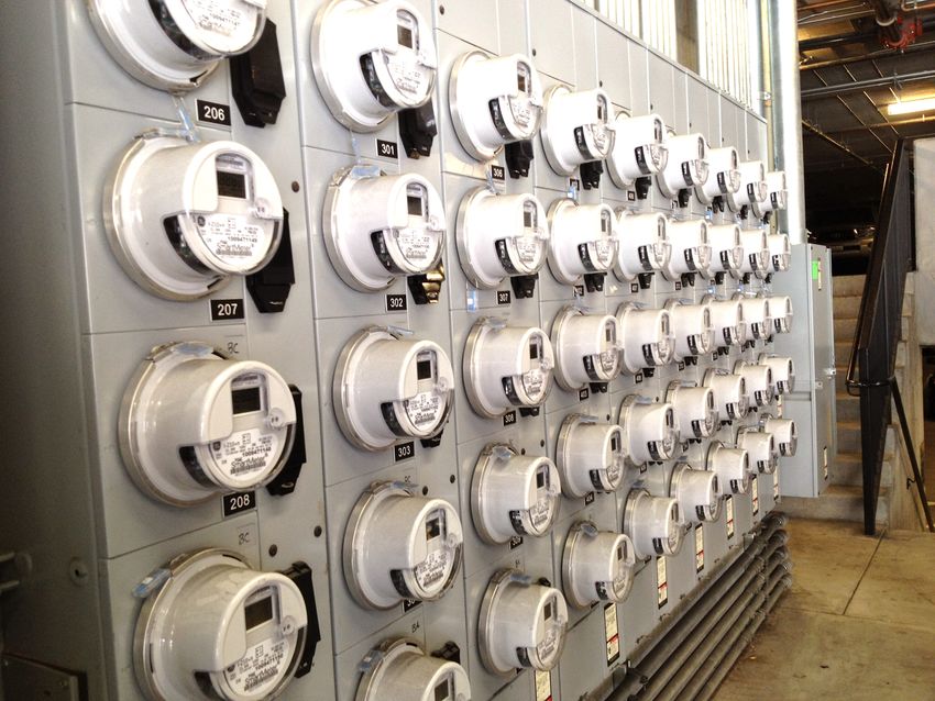
6. No Phishing Allowed!. . . . . . . . . . . . . . . . . . . . . . . . . . . . . . . . . . . . . . . 47
The Phishing Attack 47
The No-Phishing-Allowed Anomaly Detector 49
How the Model Works 50
Putting It All Together 51
7. Anomaly Detection for the Future. . . . . . . . . . . . . . . . . . . . . . . . . . . . . 53
A. Additional Resources. . . . . . . . . . . . . . . . . . . . . . . . . . . . . . . . . . . . . . . . 57
iv | Table of Contents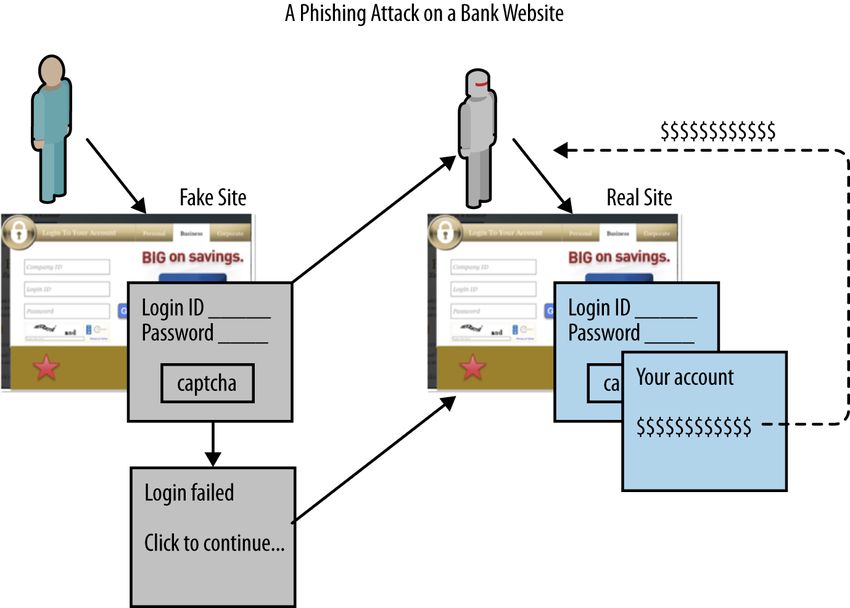
CHAPTER 1
                 Looking Toward the Future

Everyone loves a mystery, and at the heart of it, that’s what anomaly
detection is—spotting the unusual, catching the fraud, discovering the
strange activity. Anomaly detection has a wide range of useful appli‐
cations, from banking security to natural sciences to medicine to mar‐
keting. Anomaly detection carried out by a machine-learning program
is actually a form of artificial intelligence. With the ever-increasing
volume of data and the new types of data, such as sensor data from an
increasingly large variety of objects that needs to be considered, it’s no
surprise that there also is a growing interest in being able to handle
more decisions automatically via machine-learning applications. But
in the case of anomaly detection, at least some of the appeal is the
excitement of the chase itself.

                                                                         1
Figure 1-1. Finding anomalies is the detective work of machine
learning.

When are anomaly-detection methods a good choice? Unlike fictional
detective stories, in anomaly detection, you may not have a clear sus‐
pect to search for, and you may not even know what the “crime” is. In
fact, one way to think about when to turn to anomaly detection is this:
Anomaly detection is about finding what you don’t know to look for.
You are searching for anomalies, but you don’t know what their char‐
acteristics will be. If you did, you could use a different form of machine
learning, called classification, or you would just write specific rules to
find the anomalies. But that’s not generally where you start.
Classification is a form of supervised learning where you have exam‐
ples of each kind of thing you are looking for. You apply a learning
algorithm to these examples to build a model that can use features of
new data to classify them into categories that represent each kind of
data of interest. When you have examples of normal and some number
of abnormal situations, classifers can help you mark new situations as
normal or abnormal. Even when you know about some kinds of
anomalies, it is always good to keep an eye out for new kinds that you
don’t know about. That is where anomaly detection is applied.

2   |   Chapter 1: Looking Toward the Future
So you use the unsupervised-learning approach of anomaly detection
when you don’t know exactly what you are looking for. Anomaly de‐
tection is a discovery process to help you figure out what is going on
and what you need to look for. The anomaly-detection program must
discover interesting patterns or connections in the data itself, and the
detector does this by first identifying the most important aspect of
anomaly detection: finding what is normal. Once your model does that,
your machine-learning program can then spot outliers, in other
words, data that falls outside of what is normal.
Anomalies are defined not by their own characteristics, but in contrast
to what is normal. You may not know what the anomalies will look
like, but you can build a system to detect them in contrast to what
you’ve discovered and defined as being a normal pattern. Note that
normal in this context includes all of the anomalies that you already
know about and have accounted for using a classifier. The outliers are
only those events that don’t match what you already know. Consider
this way to think about the problem: anomaly in this context just
means different than expected—it does not refer to desirable or un‐
desirable. You may know of certain types of events that are somewhat
unusual and require attention, perhaps certain failures in a system. If
these occur sufficiently often to be well characterized, you can use a
classifier to catalog them as problems of a particular type. That’s a
somewhat different goal than true anomaly detection where you are
looking for events that are rare relative to what is expected and that
often are surprising, or at least undefined ahead of time.
Together, anomaly detection and classification make for a useful pair
when it comes to finding a solution to real-world problems. Anomaly
detection is used first—in a discovery phase—to help you figure out
what is going on and what you need to look for. You could use the
anomaly-detection model to spot outliers, then set up an efficient
classification model to assign new examples to the categories you’ve
already identified. You then update the anomaly detector to consider
these new examples as normal and repeat the process. This idea is
shown in Figure 1-2 as one way to use anomaly detection.

                                              Looking Toward the Future   |   3
Figure 1-2. Use anomaly detection when you don’t know what to look for. Sometimes this discovery process makes a useful preliminary stage to define the categories of interest for a classifier. Anomaly detection, like classification, is not new, but recently there has been an increased interest in using it. Fortunately, there also are new approaches to carrying it out effectively in practical settings; much more accurate and sophisticated methods are now available. Some of the biggest changes have to do with being able to handle anomaly detection at huge scale, in real time. We will describe some approaches that can help, especially when using a realtime distributed file system. We will focus particularly on approaches that have demon‐ strated, practical, and simple implementations. The move from specialized academic research to methods that are useful for practical machine learning is happening in response to more than just an increase in the volume of available data—there is also a great increase in new types of data. For example, many new forms of sensors are being deployed. Smart meters monitor energy usage in businesses and residential settings, reporting back every few minutes. This information can be used individually or looked at as a group from a particular geographical location. 4 | Chapter 1: Looking Toward the Future
Figure 1-3. This wall of smart meters reports a granular view of ener‐
gy usage for a utility company. Sensor data is becoming a huge source
of valuable information that can be analyzed through machine learn‐
ing techniques such as anomaly detection.

Industrial equipment such as drilling rigs and manufacturing tools use
sensors to report on a wide range of parameters. The advances in
medical device sensors are astounding. Radio-frequency identifica‐
tion (RFID) tags are also commonplace on merchandise in retail
stores, in warehouses, or even on your cat. Data provided by these
sensors and other sources range from simple identification signals to
complex measurements of temperature, pressure, vibrations, and
more.
How can reporting from all these interconnected objects be used?
Collectively, these objects begin to make up the Internet of Things
(IoT). Relationships between objects and people, between objects and
other objects, conditions in the present, and histories of their condi‐
tion over time can be monitored and stored for future analysis, but
doing so is quite a challenge. However, the rewards are also potentially
enormous. That’s where machine learning and anomaly detection can
provide a huge benefit.

                                              Looking Toward the Future   |   5
Analysts predict that the number of interconnected devices in the In‐ ternet of Things will reach the tens of billions less than a decade from this writing. Machine-learning techniques will be critical to our un‐ derstanding of what the signals from devices are telling us. As we collect and analyze more data from sensors, we achieve a more granular view of how our systems are functioning, which in turn gives us the opportunity for a greater awareness of when things change for better or for worse. Not only is there a growing need for more accurate anomaly detection, there is also a growing desire for new and more efficient ways to “cut to the chase” in order to be able to put anomaly detection to work in practical, real-world settings. Practical anomaly detection is more than just selecting the right algorithm and having the technical expertise to build the system—it also means finding sol‐ utions that take into account realistic limitations on resources, sched‐ uling demands including time-to-value to make the projects cost ef‐ fective, and correct understanding of business goals. In this publication, we show you the underlying ideas of why anomaly detection works and what it’s good for. We explore then idea of finding what is normal, deciding how to measure things that are far from nor‐ mal and how far that must be to be considered an outlier (Chapters 2 and 3). We provide a new method to do this (t-digest) and look at how it can be applied in very simple systems (Chapter 3) and also in more complex systems (Chapters 4 and 5). Throughout this report, we strongly recommend the use of adaptive, probabilistic models for predicting what is normal and how to contrast that to what is observed. One of our topics in Chapter 4 dabbles in deep learning with a time-series example, or at least dips its toe into the shallow end of that pool. Although this is an advanced concept, the execution of it in our example is surprisingly simple—no advanced math required. Chapter 5 provides some very practical ways to model a system with sporadic events, such as website traffic or e-commerce purchases. In Chapter 6, we provide a practical illustration of many of the basic concepts in the form of detecting a phishing attack on a secure website. Let’s see how all this works. 6 | Chapter 1: Looking Toward the Future
CHAPTER 2
    The Shape of Anomaly Detection

The exciting thing about anomaly detection is the sense of discovery.
You need a program that can spot what is unusual, so anomaly-
detection models are on the lookout for the outliers. To get a sense of
how this works, try a simple human-scale example, such as the one
shown in Figure 2-1. Can you spot an outlier?

Figure 2-1. Can you spot an anomaly in this data?

Despite the fact that there is apparent noise in the data of the horizontal
line shown in Figure 2-1, when you see data like this, it’s fairly easy to
see that the large spike appears to be an outlier. But is it?

                                                                          7
What happens when you have a larger sample of data? Now your per‐
ception changes. What had appeared to be an anomaly turns out to be
part of a regular and even familiar pattern: in this case, the regular
frequency of a normally beating heart, recorded using an EKG, as
shown in Figure 2-2.
Figure 2-2. Normal heartbeat pattern recorded in an EKG. The spikes
that had, in isolation, appeared to be anomalies relative to the hori‐
zontal curve are actually a regular and expected part of this normal
pattern.
There’s an important lesson here, even in this simple small-scale
example:
Before you can spot an anomaly, you first have to figure out what
“normal” is.
Discovering “ normal” is a little more complicated than it sounds,
especially in a complex system. Often, to do this, you need a machine-
learning model. To do this accurately, you also need a large enough
sampling of data to get an accurate representation. Then you must find
a way to analyze the data and mathematically define what forms a
regular pattern in your training data.
Finding “Normal”
Let’s think for a moment about the basic ideas that underlie anomaly
detection, including the idea of discovering what is to be considered
a normal pattern of behavior. One basic but powerful way to do this
is to build a probabilistic model, an idea that we progressively develop
8 | Chapter 2: The Shape of Anomaly Detectionhere and in Chapters 3 through 6. A good way to think about this is
in terms of mathematic symbols, but in case that’s not your preference,
consider the key ideas through this thought experiment.
Suppose you are studying birds in a particular location, and you ob‐
serve, identify and count how many birds and of what species pass by
a particular observation point over the course of days. An entirely
made-up example of what these observations might look like is shown
in Table 2-1.
Table 2-1. Bird watching provides a simple thought experiment to
show how a probabilistic model works. Once a new species was ob‐
served, we watched for it on subsequent days. The synthetic data of
this simplified example helps you think about how, based on the ob‐
servations you’ve made, you could build a model to predict several
things about what you expect to observe on Day x.
Species Day 1 Day 2 Day 3 Day 4 Day 5 Day x
A 33 17 21 31 18 ?
B 7 1 2 3 3 ?
C 3 3 2 1 1 ?
D 5 3 0 0 0 ?
E 13 13 8 7 9 ?
F 1 0 0 0 0 ?
G 1 0 0 0 0 ?
H 3 3 5 1 6 ?
I - 2 1 0 1 ?
J - 1 0 0 0 ?
K - - - 1 0 ?
L - - - - 1 ?
Next - - - - - ?
Some species occur in fairly high numbers each day, and these species
tend to be observed every day. Several species occur much less com‐
monly. New species are seen almost every day, at least this early in the
experiment. You can predict several things for a subsequent day (or
short series of days):
• How many total birds you expect to see
• How many species you expect to see
• How many birds of each species will fly by
Finding “Normal” | 9• How many new, previously unobserved, species will be seen This prediction is nicely captured in the form of a probabilistic model. It assumes that all things (species) have at least some likelihood to occur, that some are more likely than others, and some are extremely rare (or not yet observed), and so the estimate of their likelihood will be a very small value. You can even predict how many new species you might expect on a given day, even if you cannot predict which species they will be. You can assign a probability for each event or type of event and thus describe in probabilistic terms what you estimate to be “nor‐ mal.” If you enjoy math, read this description of a probabilistic model of “normal”… For those of you who prefer a mathematical way to describe things, read on. For the rest of you, just skip this description and go to the next section. Suppose that our best guess of the probability of some observation i from the set of all possible observation is πi. The true underlying probability is pi. Because our model is a probabilistic model, the values πi are constrained by definition in the following way: What this means is that if we make πi large for some i, then we have to make it smaller for some other i. Moreover, since the πi have to all be non-negative, smaller means closer to zero but never less than zero. The very deep mathematical inference that we can draw here is that if we make the average value of –log πi as small as possible, then we can prove that the estimated probabilities, πi, will be as close as possible to the true underlying probabilities, pi. In fact: where the maximum is only achieved if πi = pi for all i. A rare event is expected to have a small value for πi, and thus the value for –log πi will all be a relatively large positive number. You might think 10 | Chapter 2: The Shape of Anomaly Detection
that creates a problem, making the average –log πi large when our best
estimate of probabilities would need for it to be small. But remember
that the average is computed by weighting things according to their
probability, so that each rare thing will only have a small contribution.
Depending on the details of your data and what they represent, there
are various ways to prepare data for use in such a model and a variety
of appropriate algorithms from which to choose. We will describe
several options in upcoming chapters.

Human Insight Helps
Discovering a normal pattern requires more than just a good machine-
learning model. Part of the process of discovering normal involves
human insight: you must interact with the modeling process to decide
what makes sense in your own situation. The example of a single
heartbeat shown in Figure 2-2 makes this point. In an abstract sense,
the spike is anomalous as compared to the rest of the data. In our
example, just collecting more data, such as what’s shown in a full EKG,
is more than enough to recognize that the spikes are a normal part of
the heart function, but before seeing more data, an expert who knew
it was an EKG being analyzed would also tell you that the spike was
not an anomaly.
Our bird-watching thought experiment can also illustrate this point.
Suppose you observe a brown pelican—is this to be expected? A do‐
main expert would tell you yes, if you live near a coastal region of North
America, or no if you live for instance in the inland state of North
Dakota. Similarly, cedar waxwings are not seen for most of the year in
California but sightings suddenly become relatively commonplace
during a short period of migration. Of course the historical data would
reveal these fluctuations, and this is just an analogy, but the point is
that human insight from someone with domain knowledge is a val‐
uable resource to put a probabilistic model into the proper context.
Continuing with our bird-watching thoughts, human experience
might also inform you that some sequential events tend to be related.
If you see one pelican fly by, it’s reasonable to expect several more
almost immediately because they often fly in a sort of squadron. But
you would not expect a couple of hundred pelicans in rapid succession.
This knowledge suggests to us not only that sequential measurements
may not be entirely independent—an important concept—but also

                                                   Human Insight Helps   |   11
that models may require several levels of complexity to be really ac‐ curate predictions of real-world events. So the first step in anomaly detection—using your model to discover what is normal—also requires human insight both to structure the model mathematically as well as to interpret what aspect of a pattern is of interest and whether or not it represents a reasonable view of a normal situation. In building a machine-learning model for anomaly detection, you have to identify the best choice of data, figure out how to put it into a form acceptable to your algorithm and then acquire enough data for training your model. In other words you will use data initially to let the model discover patterns that you will then need to interpret in order to determine the baseline or normal situation. This may require a number of adjustments to the algorithm you use before you end up with something that makes sense. The more you know about the sit‐ uation being investigated, the more easily and accurately you can de‐ cide when your model has achieved the first goal of anomaly detection by finding what is normal. Finding Anomalies A second level of human insight is needed once you’ve established what is normal and begin to look for what is anomalous. For our EKG example, anomalous behavior is not the fact that there are spikes but the observation that their frequency fluctuates during an episode of abnormal heart behavior, as seen in the data displayed in Figure 2-3. 12 | Chapter 2: The Shape of Anomaly Detection
Figure 2-3. Anomalies in the frequency of the heartbeat show up as
unevenly spaced spikes such as those between approximately 1206
and 1210 seconds in this EKG.

Figures 2-2 and 2-3 just illustrate the point that the basis for anomaly
detection is to establish what is normal and then compare new events
to that pattern or model. This two-step process can be done in a variety
of ways from very simple models of fairly straightforward systems that
use an assigned threshold to send alerts for potential anomalies (as
described in Chapter 3) or more sophisticated models that are adaptive
and can deal with complex or shifting situations (as explained in
Chapters 4 through 6. In all of these cases, you are comparing observed
behavior to what has been defined as normal.
Back to our bird-watching example: when the observations show ei‐
ther a big decrease in the overall number of common birds or the
appearance of a large number of very rare birds, your model should
flag the change as being anomalous.

Once again, if you like math, this description of
anomalies is for you…
Thinking in terms of a probabilistic model, very rare, anomalous
events will be assigned a much lower probability value than normal
events during training. As a result, during an anomaly when we ob‐
serve these rare events, the anomaly score will be large precisely be‐
cause our estimate of their probability is very low.
Because an anomalous event has a lower probability value than those
usually observed, the anomaly score, which is the negative log of the

                                                   Finding Anomalies   |   13
probability value, –log πi, will be larger, possibly much larger than
usual. In other words, the anomaly score will be farther from the ideal
maximum of zero. This increase suggests that our model’s estimation
of normal is less well matched to actual anomalous events—thus high‐
lighting the occurrence of outliers.
Take-Home Lesson: Key Steps in Anomaly Detection
The overall message here is broadly applicable to different types of
anomaly detection, regardless of the complexity of the system and the
choice of algorithms that are used. These steps form a general guide‐
line to goals when you are trying to build your own anomaly detector.
Ask yourself these questions:
• What is normal?
• What will you measure to identify things that are “far” from
normal?
• How far is “far”, if something is to be considered anomalous?
A Simple Approach: Threshold Models
You must experiment to determine at what sensitivity you want your
model to flag data as anomalous. If it is set too sensitively, random
noise will get flagged, and with huge amounts of data, it will be essen‐
tially impossible to find anything useful beyond all the noise.
Even if you’ve adjusted the sensitivity to a coarser resolution such that
your model is automatically flagging actual outliers, you still have a
choice to make about the level of detection that is useful to you. There
always are trade-offs between finding everything that is out of the or‐
dinary and getting alarms at a rate for which you can handle making
a response. These considerations, as well as a useful new way to set a
good threshold, are the topic of Chapter 3.
14 | Chapter 2: The Shape of Anomaly DetectionCHAPTER 3
Using t-Digest for Threshold
Automation
The most common form of anomaly detector in use today is a
manually-set threshold alarm to send an alert for possible anomalies.
Input to such an alarm is a numerical measurement of some kind. The
basic idea in this case is that whenever this measurement exceeds a
threshold that you have set, possibly for a certain amount of time, an
alarm is sounded.
This simple approach can work fairly well if the system being observed
has a simple pattern of well-understood measurements, and the num‐
ber of different kinds measurements is not enormous. But this ap‐
proach can become quite difficult to carry out effectively if you have
a large number of measurements with behaviors that you do not un‐
derstand very well. As it turns out, that situation—a large number of
measurements in a system that is either unpredictable or otherwise
not well defined—is commonly encountered in real-world settings of
interest. That’s one reason we need some new ways to approach anom‐
aly detection.
A good first step in improving these systems is to change the way that
the threshold is set. Let’s think about the goal for a threshold and how
it can be optimized. Any particular value for a threshold will detect
some fraction of the anomalies that you are trying to find, and if you
have chosen the threshold well, that fraction of anomalies hopefully
will be large. At the same time, this threshold most likely will some‐
times trigger false alarms, in cases in which normal noise in the data
is detected erroneously as being a true anomaly. Once again, if the
15system is built well and an appropriate threshold was chosen, the number of false alarms will be small. This trade-off between catching anomalies but trying to avoid too many false positives is what you are trying to optimize as you set the threshold. If you are trying to detect anomalous positive deviations of the meas‐ urement you are collecting, then increasing the threshold will decrease the fraction of measurements that are false alarms (the false positive rate) but will also decrease the fraction of true anomalies we find (the true positive rate). Conversely, decreasing the threshold will have the opposite effect, finding more of the anomalies we are targeting but at the price of an increase in false positives. This decision is a trade-off between the two kinds of error: false positives and false negatives. The idea of these trade-offs is illustrated in Figure 3-1. Figure 3-1. The idea of trade-offs in setting the threshold for alarm. The gray line is noisy but non-anomalous data. The black horizontal line shows the mean of the data—a crude model. The three circles are true anomalies. Where would you set a threshold to detect the anomalies without excessive false positives? You could set a threshold to get a perfect record for catching anomalies, but then you’ve created a large and undesirable side effect of also get‐ ting a lot of what you don’t want (false positives). This is a standard challenge in risk management that applies to much more than just monitoring systems—it also applies to many societal decisions. 16 | Chapter 3: Using t-Digest for Threshold Automation
The Philosophy Behind Setting the Threshold
The question you face is, “How many false positives are acceptable and
what is the cost of possibly missing some real anomalies?” Roughly
speaking, people fall into two broad groups in their goals for optimiz‐
ing the threshold. These strategies are depicted in Figure 3-2. On one
side are those for whom the major objective is to detect a very large
fraction of anomalies because the penalty for missing any of them is
great. An example might be a medical life-support device for which
very sensitive detection of anomalies is important.

Figure 3-2. Goals for anomaly detection vary, and that in turn affects
how you select a threshold. Anomaly-driven situations are those in
which you have a required rate of detection and must estimate the
number of false alarms in order to budget for that. Budget-driven
anomaly detection occurs when you have a limited budget for re‐
sponse, and you must determine how many anomalies and false
alarms you can handle within that budget, setting the threshold to
match.

You could set the anomaly detection threshold very low in order to
catch most or all anomalies, but this can result in a high rate of false
positives. Dealing with false alarms also has a cost, however. You must
have sufficient resources to respond to the alarms and determine
whether or not they are false positives. Too many false alarms becomes
a distraction, wastes time, and potentially overwhelms the human who
needs to respond. This person could become habituated to the alarm,
raising the danger that they will not respond appropriately to a true

                               The Philosophy Behind Setting the Threshold   |   17
anomaly—it’s a case of the danger of “crying wolf ” too often. Even so, in a system with a high penalty for missed anomalies, you still have to choose the threshold to reduce the rate of missed anomalies to the required level. Given that threshold, you then calculate what you must budget in time and expense to handle anomalies and the many false positives you are likely to have. In contrast is the budget-driven philosophy in which you have to work with a fixed budget for dealing with all alarms. In this case, your budget drives your choice of threshold, even if it means missing some true anomalies. For a whimsical example, consider measurements in a chocolate candy factory. The measurement in question might be the input and output amount of chocolate, or how many chocolate nuggets are dropped in each bag, or the ratio of chocolate and peanuts for each piece of candy. The anomalies you would like to detect might include temperature fluctuations of the melted chocolate, problems with vis‐ cosity, or errors in the swing of a mechanical arm that extrudes a stream of chocolate. While it might seem heartbreaking to your loyal customers to end up with a charred taste because the system overhea‐ ted the chocolate one day, it’s not life-threatening. In this case, you are likely to be driven by a trade-off of the cost of dealing with alarms to alert you to fluctuations versus the potential threat to producing a batch of candy that will disappoint your customers. Ideally, in general, you want to have as high a true positive rate as you can, but you also have a maximum number of false positives that you can afford to deal with. You must therefore choose your threshold to control the total alarms in a given time period. Theoretically, you should be able to set this threshold by examining the distribution of the measurement under normal conditions and picking a value of the threshold to give the desired rate of alarms. This assumption is an especially good fit for the budget-driven situations. As an example, suppose that we have a measurement that is made once per second, and we are willing to investigate three false positives per month. We will have about 3 million measurements per month, so we can accept about one false positive per million measurements. In that case, the threshold should be set to roughly the 99.9999th percentile. That action may sound easy, but incrementally calculating an extreme quantile accurately with limited memory can be difficult, especially if you need to do this for a large number of related situations. In the next section, we will describe how to use a new algorithm, t-digest, to es‐ timate extreme quantiles on large data sets in an online fashion. 18 | Chapter 3: Using t-Digest for Threshold Automation
Another consideration is that, in practice, successive measurements
are often highly correlated. (Remember the squadron of pelicans we
mentioned in the analogy in Chapter 2?) When measurements exhibit
such correlations, we may want to consider short batches of inputs
instead of individual points when setting the threshold. In the example
above with one measurement per second, we might actually only have
the equivalent of one independent measurement every 5 minutes and
thus would consider 5-minute batches instead of individual points. In
that case, to get the desired 3 alarms per month, we want to allow one
5-minute batch or about 300 measurements above the threshold per
million measurements, and the threshold should be set to the 99.97th
percentile. The measurements that exceed the threshold will occur in
bunches due to correlation, and the total number of alerts we have to
respond to will be much less than the number of measurements above
the threshold.
In either case, percentiles are a very natural scale for talking about the
threshold setting. Translating a percentile into a threshold can be
tricky with limited memory and time, however. That’s where t-digest
can help.

Using t-Digest for Accurate Calculation of
Extreme Quantiles
The data structure known as t-digest was developed by one of the
authors, Ted Dunning, as a way to accurately estimate extreme quan‐
tiles for very large data sets with limited memory use. This capability
makes t-digest particularly useful for selecting a good threshold for
anomaly detection. The t-digest algorithm is available in Apache Ma‐
hout as part of the Mahout math library. It’s also available as open
source at https://github.com/tdunning/t-digest and has been published
to Maven Central. The t-digest algorithm has been picked up by several
other projects, including Elasticsearch and stream-lib.
One of the advantages of t-digest is accuracy, especially for extreme
quantiles; another is making the problem less cumbersome by re‐
quiring limited amounts of memory. Instead of having to sort a large
number of samples to estimate a quantile of interest, an incoming sig‐
nal can be analyzed in an online fashion using a t-digest to find the
threshold corresponding to any quantile. This process is shown in
Figure 3-3. The threshold is selected in terms of which percentile of
the distribution of the incoming signal is desired. In this case, a thresh‐

                     Using t-Digest for Accurate Calculation of Extreme Quantiles   |   19
old of 99.97% has been selected. To alert us of negative deviations, the sign of the comparison would be reversed, and a low percentile would be selected instead of a high one. Figure 3-3. Using the t-digest to set a threshold. The incoming signal (x) is routed to the t-digest to estimate the threshold (h) as a quantile. New incoming data is compared to this threshold. Issues with Simple Thresholds The basic idea behind any anomaly detector is that we are building a model of the input to the detector—our estimation of “normal”— looking for deviations from that model. The model for the threshold- based anomaly detector is based on an assumption that the incoming signal has a nearly stationary and simple distribution so that a partic‐ ular percentile will always be at a particular point. If this assumption doesn’t hold, and often it does not, then the threshold as computed by the t-digest will result in the rate of true and false positives to vary as the distribution of the signal changes. Figure 3-4 shows an example of a signal that exhibits this problem. 20 | Chapter 3: Using t-Digest for Threshold Automation
Figure 3-4. A non-stationary distribution can make it hard to see
some anomalies using a simple threshold.

With any kind of simple threshold detector, the anomaly at A in
Figure 3-4 will be detected easily, but the anomaly at B will not, even
though they are both much larger than the noise level.
Clearly, we need a more nuanced and adaptive kind of model to handle
this sort of problem. We will explore how to do this in the next chapter.

                                           Issues with Simple Thresholds   |   21
CHAPTER 4
More Complex, Adaptive Models
As we saw in the previous chapter, it is relatively easy to build the very
simplest anomaly detector that looks for deviations from an ideal val‐
ue. Tools like the t-digest can help by analyzing historical data to ac‐
curately find a good threshold. Statistically, such a system is building
a model of the input data that describes the data as a constant value
with some additive noise. For a system like most of the ones we have
seen so far, the model is nearly trivial, but it is a model nonetheless.
But what about the more complicated situations, such as the one
shown at the end of the last chapter in Figure 3-3? Systems that are
not stationary or that have complicated patterns even when they are
roughly periodic require something more than a simple threshold de‐
tector. And what happens when conditions change?
What is needed is an adaptive machine-learning model for anomaly
detection. In Chapter 2 we discussed the idea of a probabilistic model
that is trained using histories of past events to estimate their likelihood
of occurrence as a way to describe what is normal. This type of model
is adaptive: as small fluctuations occur in the majority of events, our
model can adjust its view of “normal” accordingly. In other words, it
adapts to reasonable variations. Back to our bird-watching analogy, if
our bird detector is looking for unusual species (“accidentals” in bird-
watching jargon) or significant and possibly catastrophic changes in
the population of normal species, we might want our model to be able
to adjust to small changes in the local population that respond to slight
shifts in weather conditions, availability of seeds and water, or exces‐
sive activity of the neighbor’s cat. We want our model to be adaptive.
23Conceptually, it is relatively easy to imagine extending the constant threshold model of Chapter 3 by allowing the mean value to vary and then set all thresholds relative to that mean value. Statistically speak‐ ing, what we are doing is describing our input as a time-varying base value combined with additive noise that has constant distribution and zero mean. By building a model of exactly how we expect that base value to vary, we can build an anomaly detector that produces an alert whenever the input behaves sufficiently differently from what is expected. Let’s take a look at the EKG signal that we talked about in Chapter 2 of this report. The pulses in the EKG that record the heartbeats of the patient being measured are each highly similar to one another. In fact, substantial changes in the shape of the waveforms in the EKG often indicate either some sort of physiological problem or equipment mal‐ function. So the problem of anomaly detection in an EKG can be viewed as the problem of how to build a model of what heartbeats should look like, and then how to compare the observed heartbeats to this ideal model. If the model is a good one—in other words a good estimate of normal heart behavior—then a measurement of error for observed behavior relative to this ideal model will highlight anomalous behavior. If the magnitude of the error stands out, it may be a flag that highlights irregular heartbeats or a failure in the monitor. This ap‐ proach can work to find anomalies in a variety of situations, not just for an EKG. To understand this mathematically (just stay with us), think back to Chapter 2, in which we stated that anomaly detection involves mod‐ eling what is normal, looking for events that lie far from normal, and having to decide how to determine that. In the type of example de‐ scribed in this current chapter, we have a continuous measurement, and at any point in time, we have a single value. The probabilistic model for “normal” in this situation involves a sum of a base value plus random noise. We can estimate the base value using our model, and subtracting this from our observational input data leaves the random noise, which is our reconstruction error. According to our model, the error noise has an average value of zero and stationary distribution. When the remaining noise is large, we have an anomaly, and t-digest can decide what we should consider a large value of noise to be. 24 | Chapter 4: More Complex, Adaptive Models
Windows and Clusters
We still have the challenge of finding an approachable, practical way
to model normal for a very complicated curve such as the EKG. To do
this, we are going to turn to a type of machine learning known as deep
learning, at least in an introductory way. Here’s how.
Deep learning involves letting a system learn in several layers, in order
to deal with large and complicated problems in approachable steps.
With a nod toward this approach, we’ve found a simple way to do this
for curves such as the EKG that have repeated components separated
in time rather than superposed. We take advantage of the repetitive
and separated nature of an EKG curve in order to accurately model its
complicated shape.
Figure 4-1 shows an expanded view of two heartbeats from an EKG
signal. Each heartbeat consists of several phases or pulses that corre‐
spond to electrical activity in the heart. The first part of the heartbeat
is the P wave, followed by the QRS complex, or group of pulses, and
then the T wave. The recording shown here was made with a portable
recording device and doesn’t show all of the detail in the QRS complex,
nor is the U wave visible just after the T wave. The thing to notice is
that each wave is strikingly similar from heartbeat to heartbeat. That
heart is beating in a normal pattern.
To build a model that uses this similarity, we use a mathematical trick
called windowing. It’s a way of dealing with the regular but complex
patterns when you need to build a model that can accurately predict
them. This method involves extracting short sequences of the original
signal in such a way that that the short sequences can be added back
together to re-create the original signal.

                                                  Windows and Clusters   |   25
Figure 4-1. An EKG signal is comprised of components that are com‐ plex but highly repetitive. The first step of our analysis is to do windowing to break up the larger pattern into small components. Figure 4-2 shows how the EKG for these two heartbeats are broken up into a sequence of nine overlapping short signals. As you can see, several of these signals are similar to each other. This similarity can be exploited to build a heartbeat model by aligning and clustering all of the short signals observed in a long re‐ cording. In this example, the clustering was done using a ball k-means algorithm from the Apache Mahout library. We chose this algorithm because our sample data here is not huge, so we could do this as an in- memory operation. With larger data sets, we might have done the clustering with a different algorithm, such as streaming k-means, also from Mahout. The clustering operation essentially builds a catalog of these shapes so that the original signal can be encoded by simply recording which shape from the catalog is used in each time window, along with a scal‐ ing factor for each shape. 26 | Chapter 4: More Complex, Adaptive Models
Figure 4-2. Windowing decomposes the original signal into short seg‐
ments that can be added together to reconstruct the original signal.

By looking at a long time series of data from an EKG, you can construct
a dictionary of component shapes that are typical for normal heart be‐
havior. Figure 4-3 shows a selection of 64 out of 400 shapes from a
dictionary constructed based on several hours of a real EKG recording.
These shapes clearly show some of the distinctive patterns found in
EKG recordings.

                                                Windows and Clusters   |   27
Figure 4-3. Dictionary of component shapes. Clustering finds the most commonly used signal shapes for reconstructing a representation of normal heartbeats. Matches with the Windowed Reconstruction: Normal Function Now let’s see what happens when this technique is applied to a new EKG signal. Remember, the goal here is to build a model of an observed signal, compare it to the ideal model, and note the level of error be‐ tween the two. We assume that the shapes used as components (the dictionary of shapes shown in Figure 4-3) are accurate depictions of a normal signal. Given that, a low level of errors in the comparison between the re-constructed signal and the ideal suggests that the ob‐ served signal is close to normal. In contrast, a large error points to a mismatch. This is not a test of the reconstruction method but rather a test of the observed signal. A mismatch indicates an abnormal signal, and thus an anomaly in heart function. Figure 4-4 shows a reconstruction of an EKG signal. The top trace is the original signal, the middle one is the reconstructed signal, and the bottom trace shows the difference between the first two. This last sig‐ nal shows how well the reconstruction encodes the original signal and is called the reconstruction error. 28 | Chapter 4: More Complex, Adaptive Models
Figure 4-4. Reconstruction of normal pattern for heartbeats using
windowing and clustering. The reconstruction error (bottom trace)
for an EKG signal (top trace) is computed by subtracting the recon‐
structed signal (middle trace) from the original. Notice that the recon‐
struction error (bottom trace) is small and relatively uniform.

As long as the original signal looks very much like the signals that were
used to create the shape dictionary, the reconstruction will be very
good, and the reconstruction error will be small. The dictionary is thus
a model of what EKG signals can look like, and the reconstruction
error represents the degree to which the signal being reconstructed
looks like a heartbeat. A large reconstruction error occurs when the
input does not look much like a heartbeat (or, in other words, is
anomalous).
Note in Figure 4-4 how the reconstruction error has a fixed baseline.
This fact suggests that we can apply a thresholding anomaly detector
as described in Chapter 3 to the reconstruction error to get a complete
anomaly detector. Figure 4-5 shows a block diagram of an anomaly
detector built based on this idea.

                   Matches with the Windowed Reconstruction: Normal Function   |   29
Figure 4-5. Signal reconstruction error from an auto-encoder can be used to find anomalies in a complex signal. Input signal x is analyzed using an encoder, which reconstructs x using a model in the form of a shape dictionary to produce a reconstructed signal x’. The difference, x-x', is the reconstruction error δ. Comparing δ to a threshold h gives us an alarm signal when the encoder cannot reconstruct x accurately as indicated by a large reconstruction error δ. Essentially what is happening here is that the encoder can only repro‐ duce very specific kinds of signals. The encoder is used to reduce the complex input signal to a reconstruction error, which is large when‐ ever the input isn’t the kind of signal the encoder can handle. This reconstruction error is just the sort of stationary signal that is appro‐ priate for use with the methods described in Chapter 3, and so we can use the t-digest on the reconstruction error to look for anomalies. Mismatches with the Windowed Reconstruction: Anomalous Function That this approach can find interesting anomalies is shown in Figure 4-6, where you can see a spike in the reconstruction error just after 101 seconds. It is clear that the input signal (top trace) is not faithfully rendered by the reconstruction, but at this scale, it is hard to see exactly why. 30 | Chapter 4: More Complex, Adaptive Models
Figure 4-6. Reconstruction for a heart signal displaying anomalous
behavior. Top trace is the original EKG signal. The bottom trace
shows the reconstruction error that is computed by subtracting the re‐
constructed signal (middle trace) from the original. Notice the spike in
the error at just past 101 seconds. That error spike indicates that the
reconstruction shown in the middle panel was unable to reproduce
that section of the original signal shown at the top.

If you expand the time scale, however, it is easy to see what is hap‐
pening. Figure 4-7 shows that at about 101.25 seconds, the QRS com‐
plex in the heartbeat is actually a double pulse. This double pulse is
very different from anything that appears in a recording of a normal
heartbeat, and that means that there isn’t a shape in the dictionary that
can be used to reconstruct this signal.

              Mismatches with the Windowed Reconstruction: Anomalous Function   |   31
Figure 4-7. Expanded view of the anomalous heartbeat. The anomaly (indicated by arrows) was detected by finding an unusually large re‐ construction error. This kind of anomaly detector can’t say what the anomaly is. All it can do is tell us that something unusual has happened. Expert human judgment is required for the interpretation of the physiological mean‐ ing of this anomaly, but having a system that can draw attention to where human judgment should best be applied helps if only by avoid‐ ing fatigue. Other systems can make use of this general model-based signal re‐ construction technique. The signal doesn’t have to be as perfectly pe‐ riodic for this to work, and it can involve multidimensional inputs instead of just a single signal. The key is that there is a model that can encode the input very concisely. You can find the code and data used in this example on GitHub. A Powerful But Simple Technique Note that the model used here to encode the EKG signal is fairly simple. The technique used to produce this model gives surprisingly good results given its low level of complexity. It can be used to analyze signals in a variety of situations including sound, vibration, or flow, such as what might be encountered in manufacturing or other industrial set‐ 32 | Chapter 4: More Complex, Adaptive Models
tings. Not all signals can be accurately analyzed with a model as simple
as the one used here, particularly if the fundamental patterns are su‐
perposed as opposed to separated, as with the EKG. Such superposed
signals may require a more elaborate model. Even the EKG signal re‐
quires a fancier model if we want to not only see the shape of the
individual heartbeats but also features such as irregular heartbeats.
One approach for building a more elaborate model is to use deep
learning to build a reconstruction model that understands a waveform
on both short and long time scales. The model shown here can be
extended to a form of deep learning by recursively clustering the
groups of cluster weights derived by the model described here.
Regardless, however, of the details of the model itself, the architecture
shown here will still work for inputs roughly like this one or even
inputs that consist of many related measurements.
The EKG model we discussed was an example of a system with a con‐
tinuous signal having a single value at any point in time. A
reconstruction-model approach can also be used for a different type
of system, one with multiple measurements being made at a single
point in time. An example of a multidimensional system like this is a
community water supply system. With the increasing use of sensors
in such systems that report many different system parameters, you
might encounter thousands of measurements for a single point in time.
These measurements could include flow or pressure at multiple loca‐
tions in the system, or depth measurements for reservoirs. Although
this type of system has a huge number of data points at any single time
stamp, it does not exhibit the complex dynamics of the heartbeat/EKG
example. To make a probabilistic model of such a multidimensional
water system, you might use a fairly sophisticated approach such as
neural nets or a physics-based model, but for anomaly detection, you
can still use a reconstruction error–based technique.

                                         A Powerful But Simple Technique   |   33
Looking Toward Modeling More Problematic Inputs Where this approach really begins to break down a bit is with inputs that are not based on a measurement of a value such as voltage, pres‐ sure, or flow. A good example of such a problematic input can be found in the log files from a website. In that case, the input consists of events that have a time of occurrence and some kind of label. Even though the methods described in this chapter can’t be applied verbatim, the basic idea of a probabilistic model is still the key to good anomaly detection. The use of an adaptive, probabilistic model for e-commerce log files is the topic of the next chapter. 34 | Chapter 4: More Complex, Adaptive Models
CHAPTER 5
            Anomalies in Sporadic Events

The input signals in the examples discussed in previous chapters have
all been values sampled at uniform intervals. Such signals make it easy
to talk about a reconstructed value computed by a model and the dif‐
ference between that value and the original input the reconstruction
error.
In practice, however, there are other forms of data that are important
to process for anomaly detection. One important class of such data is
known as an event stream and is usually derived from log files of one
sort or another. A key characteristic of these log files is that they record
events that occur at irregular intervals.
It is also fairly common for these events to be associated with a sym‐
bolic value such as your IP address and the URL of a web page you
visit if page views are the input of interest. Another input might be
stock trades, for which the symbolic values could include the stock
sign and be combined with the trades, price, and number of shares.
Other examples of this type of input are e-commerce purchases or
Internet packets. In each of these cases, we want to be able to detect
anomalous activity in these event streams, such as changes in the rate
or geolocation of web traffic, or perhaps the number of stock trades in
particular time periods in stock markets. Sometimes the anomaly of
interest is the absence of activity during a particular time interval, and
that can be a challenge for anomaly detection models to handle.
Because these events occur at irregular times and because they have
symbolic values rather than numerical values, it is hard to imagine
how to use the techniques from the previous chapters to find anoma‐
lies in event streams. As we will see, however, there are fundamental

                                                                          35
unifying principles that let us extend the previous methods to handle event streams. Counts Don’t Work Well You might think that doing anomaly detection on event streams is as easy as simply counting how many events occur in successive fixed- length time intervals and then considering that count as a measure‐ ment to be used with the approaches described earlier in this report. There are, however, several problems with this count-based approach. The first problem occurs because counts have inherent variation due to statistical fluctuations. This variation can make it hard to detect any small or moderate changes in system behavior without long accumu‐ lation periods. In order to detect outages reliably, we need the average counts in each period to be fairly large. We can fix this problem by making the counting interval longer to accumulate sufficient counts in each interval. But correcting this first problem creates a second problem. Waiting long enough to accumulate a large count makes it essentially impos‐ sible to detect anomalies quickly unless the event rate is really large. These ideas are illustrated in Figure 5-1. Look at the left panel in Figure 5-1, which shows frequent sampling with a short time interval. Although the rate of events being counted increases by 20% for intervals from about half to three-quarters through the 200-minute observation period, this fluctuation is hard to recognize buried in the large statistical variation inherent in small counts. 36 | Chapter 5: Anomalies in Sporadic Events
Figure 5-1. Substantial changes in rate are not easily visible for count
data with relatively low rate and short counting intervals. Left and
right panels show the same data sampled over a total of 200 minutes.
Each data point in the left panel shows the sum of counts for that one-
minute interval. In the right panel, the sampling interval was in‐
creased to 10 minutes, so there are fewer total intervals, and the count
for each one is 10 times larger. Notice that the fluctuation seen at
about half to three quarters of the way through the observation period
is much easier to see in the right panel with its longer counting inter‐
vals.

In the righthand panel, in contrast, the shift is distinctly visible, but
only at the cost of increasing the collection periods by a factor of 10.
While this makes the change visible, it also increases the time required
to detect any change, even a catastrophic one, and thus limits your
ability to respond quickly. In short, this overall situation presents a
challenging signal-to-noise problem. That’s why counts per time in‐
terval is not a good measurement to use when modeling systems that
have sporadic events.
In some systems, events arrive at such a high rate that you can have
both large counts and short intervals. It’s acceptable to use counts as
the measure for modeling in these high-rate systems, and that makes
it easy to process them using methods described in our previous chap‐
ters. Many systems aren’t like this, however, and summarizing the
event arrival data as counts leads to an unacceptable choice between
detecting small changes and responding quickly to large changes.

                                                Counts Don’t Work Well   |   37
You can also read