Lunar Seismology: A Data and Instrumentation Review
←
→
Page content transcription
If your browser does not render page correctly, please read the page content below
Space Sci Rev (2020) 216:89
https://doi.org/10.1007/s11214-020-00709-3

Lunar Seismology: A Data and Instrumentation Review

Ceri Nunn1,2 · Raphael F. Garcia3 · Yosio Nakamura4 · Angela G. Marusiak5 ·
Taichi Kawamura6 · Daoyuan Sun7,8 · Ludovic Margerin9 · Renee Weber10 ·
Mélanie Drilleau11 · Mark A. Wieczorek12 · Amir Khan13,14 · Attilio Rivoldini15 ·
Philippe Lognonné16 · Peimin Zhu17

Received: 26 March 2019 / Accepted: 17 June 2020 / Published online: 3 July 2020
© The Author(s) 2020

Abstract Several seismic experiments were deployed on the Moon by the astronauts dur-
ing the Apollo missions. The experiments began in 1969 with Apollo 11, and continued with
Apollo 12, 14, 15, 16 and 17. Instruments at Apollo 12, 14, 15, 16 and 17 remained opera-
tional until the final transmission in 1977. These remarkable experiments provide a valuable
resource. Now is a good time to review this resource, since the InSight mission is returning
seismic data from Mars, and seismic missions to the Moon and Europa are in development
from different space agencies. We present an overview of the seismic data available from

Electronic Supplementary Material
The online repository https://doi.org/10.5281/zenodo.1463224 holds the supplementary material for this
article.
B C. Nunn
     ceri.nunn@jpl.nasa.gov
1    Jet Propulsion Laboratory – California Institute of Technology, 4800 Oak Grove Drive,
     M/S: 183-501, Pasadena, CA 91109, USA
2    Ludwig Maximilian University, Munich, Germany
3    Institut Supérieur de l’Aéronautique et de l’Espace (ISAE-SUPAERO), Université de Toulouse,
     10 Ave E. Belin, 31400 Toulouse, France
4    Institute for Geophysics, John A. and Katherine G. Jackson School of Geosciences, University
     of Texas at Austin, Austin, TX, USA
5    University of Maryland, College Park, MD, USA
6    Institut de physique du globe de Paris, CNRS, Université de Paris, 75005 Paris, France
7    Laboratory of Seismology and Physics of Earth’s Interior, School of Earth and Space Sciences,
     University of Science and Technology of China, Hefei, China
8    CAS Center for Excellence in Comparative Planetology, Hefei, China
9    Institut de Recherche en Astrophysique et Planétologie, CNRS, Université de Toulouse, 14 Ave E.
     Belin, 31400 Toulouse, France
10   NASA Marshall Space Flight Center, Huntsville, AL, USA
11   Institut Supérieur de l’Aéronautique et de l’Espace SUPAERO, 10 Avenue Edouard Belin,
     31400 Toulouse, France
89 Page 2 of 39 C. Nunn et al.
four sets of experiments on the Moon: the Passive Seismic Experiments, the Active Seismic
Experiments, the Lunar Seismic Profiling Experiment and the Lunar Surface Gravimeter.
For each of these, we outline the instrumentation and the data availability.
We show examples of the different types of moonquakes, which are: artificial impacts,
meteoroid strikes, shallow quakes (less than 200 km depth) and deep quakes (around 900 km
depth). Deep quakes often occur in tight spatial clusters, and their seismic signals can there-
fore be stacked to improve the signal-to-noise ratio. We provide stacked deep moonquake
signals from three independent sources in miniSEED format. We provide an arrival-time
catalog compiled from six independent sources, as well as estimates of event time and loca-
tion where available. We show statistics on the consistency between arrival-time picks from
different operators. Moonquakes have a characteristic shape, where the energy rises slowly
to a maximum, followed by an even longer decay time. We include a table of the times of
arrival of the maximum energy tmax and the coda quality factor Qc .
Finally, we outline minimum requirements for future lunar missions to the Moon. These
requirements are particularly relevant to future missions which intend to share data with
other agencies, and set out a path for an International Lunar Network, which can provide
simultaneous multi-station observations on the Moon.
Keywords Lunar seismology · Apollo missions · Deep moonquakes ·
Shallow moonquakes · Meteoroids · Seismology · Lunar geophysical network
1 Introduction
Many seismic experiments were deployed on the Moon by the astronauts during the Apollo
missions. These experiments were part of the Apollo Lunar Seismic Experiments Package
(ALSEP). The experiments began in 1969 with Apollo 11, and continued with Apollo 12,
14, 15, 16 and 17 (Fig. 1; Table 1). The seismic instruments included passive seismometers,
a gravimeter, and geophones which were deployed in active source experiments, and then
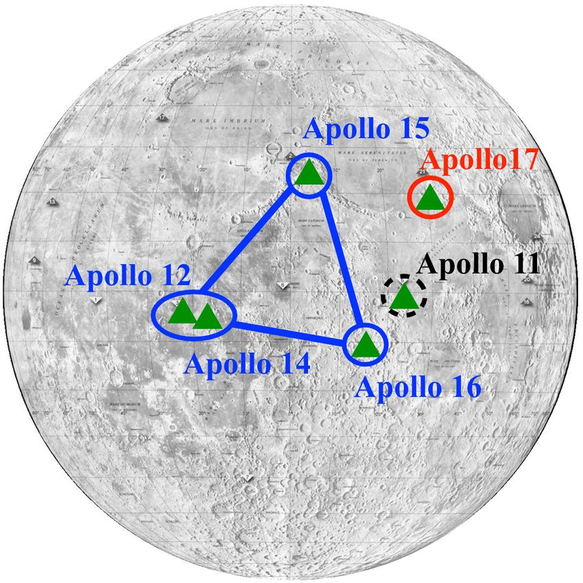
later in passive listening mode. Figure 2 shows the operating periods for each experiment.
The passive seismic stations from Apollo 12, 14, 15 and 16 remained operational until the
final transmission in 1977.
These remarkable experiments provide a valuable resource. Now is a good time to review
this resource, since there is renewed scientific interest in planetary seismology. The Mars In-
Sight mission carries a broadband seismometer and a short-period seismometer, which are
detecting marsquakes on the surface of Mars (Lognonné et al. 2019; Banerdt et al. 2020;
Giardini et al. 2020; Lognonné et al. 2020). The Seismometer to Investigate Ice and Ocean
Structure (SIIOS) project is currently being tested in sites which are analogs for the icy
moon Europa (e.g Marusiak et al. 2018; DellaGiustina et al. 2019; Marusiak et al. 2020).
12 Observatoire de la Côte d’Azur, CNRS, Laboratoire Lagrange, Université Côte d’Azur, Nica,
France
13 Institute of Theoretical Physics, University of Zurich, Zurich, Switzerland
14 Institute of Geophysics, ETH Zurich, Zurich, Switzerland
15 Observatoire Royal de Belgique, 3 Avenue Circulaire, 1050 Bruxelles, Belgium
16 Institut de Physique du Globe de Paris, CNRS, Université de Paris, Paris, 75005, France
17 China University of Geosciences, Wuhan, ChinaLunar Seismology: A Data and Instrumentation Review Page 3 of 39 89
Fig. 1 Locations of the Apollo stations on the Moon. Passive Seismic Experiments (PSE) were based at
Apollo 11, 12, 14, 15 and 16 (station 11 was only operational for one lunation). Active Seismic Experiments
(ASE) were based at Stations 14 and 16. A second active experiment, known as the Lunar Seismic Profiling
Experiment (LSPE) was based at station 17. Station 17 also included the Lunar Surface Gravimeter (LSG),
which is a source of additional passive seismic information
Table 1 Locations of the Apollo
seismic stations. Coordinates Station Coordinates
given are for the Passive Seismic Latitude Longitude
Experiments (PSE) and for the
Apollo Lunar Surface
Experiment Package (ALSEP), A11 PSE 0.67322 23.47315
which includes the active A12 PSE −3.0099 336.5752
experiments. Coordinates are A14 PSE −3.64408 342.52233
given in the DE421 mean
A14 ALSEP −3.64419 342.52232
Earth/rotation axis reference
frame (Williams et al. 2008). A15 PSE 26.13411 3.62980
From Table 5 in Wagner et al. A15 ALSEP 26.13406 3.62991
(2017) A16 PSE −8.9759 15.4986
A16 ALSEP −8.9759 15.4986
A17 ALSEP 20.1923 30.7655
Efforts in many countries indicate that an International Lunar Network of seismic stations
could be deployed on the Moon by the mid-2020s. In China, CNSA’s Chinese Lunar Explo-
ration Program deployed a lunar rover with the Chang’e 3 and Chang’e 4 missions. China is89 Page 4 of 39 C. Nunn et al.
Fig. 2 Overview of the operating periods of the Apollo seismic experiments, and data availability. Solid
blue lines indicate mainly operational instruments (with just occasional outages and data loss). Dashed lines
indicate instruments which were mostly on standby but were occasionally turned on in their listening mode.
Additional passive seismic data are available from Apollo 11 from 21 July to 3 August 1969 and again from
19 to 26 August 1969. After Nagihara et al. (2017)
planning Chang’e 5 and 6 as sample return missions (Goh 2018). In the USA, a Lunar Geo-
physical Network is one of the possible candidates for the NASA New Frontiers 5 mission
(National Research Council 2011; Shearer and Tahu 2011). The network would deploy at
least three stations containing geophysical instruments, and potentially cover the farside of
the Moon (Yamada et al. 2011; Mimoun et al. 2012). In Japan, JAXA’s SLIM (Smart Lan-
der for Investigating the Moon) is currently under development (JAXA 2018). Dragonfly is
a Titan mission which uses a rotorcraft-lander. It has been selected as NASA’s next New
Frontiers mission (APL 2019). There is considerable interest in using seismology to explore
the icy moons within our solar system (Vance et al. 2018). Lognonné and Johnson (2015)
contains a review of past and future planetary seismology.
It is important that the data from the Apollo experiments can continue to be used in the
future. Recent efforts have been made to preserve and document as much of the data as
possible, since some of the data remain on digital tapes which are deteriorating in quality.
Some tapes may have been permanently lost. The original data from the Apollo experiments
were sent to the Principal Investigator (PI) for each experiment. The PIs were responsible
for checking the data, and then archiving them. In some cases, especially where problems
were discovered with the data, the data were not archived. Some of these data have recently
been recovered (Nagihara et al. 2017). Dimech et al. (2017) analyzed thermal moonquakes
with recently rediscovered data from Apollo 17. Similarly, Nagihara et al. (2018) recovered
10% of the data missing from a heat flow experiment which ran from 1974 to 1977.
The authors of this paper are members of an international team sponsored by the In-
ternational Space Science Institute in Bern and in Beijing. The team formed to gather a
set of reference data sets and internal structural models of the Moon. This paper reviews
the available data, and the companion paper (Garcia et al. 2019) reviews lunar structural
models. Within this paper, we also outline minimum requirements for a future International
Lunar Network (ILN). If funded, NASA would provide two or more nodes, and other nations
would provide additional nodes (National Research Council 2011). These requirements are
particularly relevant to future missions which intend to share data with other agencies, and
set out a path for simultaneous multi-station observations on the Moon.Lunar Seismology: A Data and Instrumentation Review Page 5 of 39 89
2 Apollo Seismic Instruments
More than 40 years after the termination of the experiments, the Apollo data continue to
provide important insights for lunar seismology. The Apollo Lunar Surface Experiment
Packages (ALSEPs) were a unique series of in-situ geophysical experiments, which in-
cluded seismic experiments. No seismic observations have been performed on the Moon
since Apollo. The experiments included the Passive Seismic Experiment (PSE), the Ac-
tive Seismic Experiment (ASE), and the Lunar Surface Profiling Experiment (LSPE). For
decades, these data have been used to investigate the internal structure of the Moon (e.g.
Nakamura 1983; Lognonné et al. 2003; Weber et al. 2011; Garcia et al. 2011). In addi-
tion to these experiments, the Lunar Surface Gravimeter (LSG) also provides some seismic
information (Kawamura et al. 2015). In this section, we review the instrumentation.
2.1 Passive Seismic Experiments (PSE)
The Passive Seismic Experiments (PSE) were performed at Apollo 11, 12, 14, 15, and 16.
Figure 2 shows the observation period of each station. Apollo 11 functioned for only about
3 weeks. Stations 12, 14, 15 and 16 operated continuously since their deployment and func-
tioned as a seismic network until September 1977, when all the remaining experiments were
shut down. More than 13000 seismic events were cataloged using data from the mid-period
instruments during the operation of the network (Nakamura et al. 1981). The four stations
formed an almost equilateral triangle, with stations 12 and 14 at one corner (Fig. 1). The net-
work covered only a portion of the lunar nearside. This is likely one of the reasons that most
of the detected seismic events are from the lunar nearside. Each PSE station was equipped
with a 3-component (two horizontal and one vertical) mid-period displacement sensors and
a vertical-component short-period (SP). Earlier papers referred to the mid-period seismome-
ter as long-period. We use the designation mid-period to be consistent with the IRIS naming
conventions, and to better describe the capabilities of the seismometer.
The mid-period (MP) sensors were feedback displacement transducers (Sutton and
Latham 1964), with a single-pole high-pass output level stabilizer, and an 8-pole low-pass
output anti-aliasing filter for each. The SP sensor was a standard coil-magnet velocity trans-
ducer, also with a single-pole high-pass output level stabilizer and an 8-pole low-pass output
anti-aliasing filter. The feedback signals from the MP sensors were recorded as tidal (TD)
signal outputs.
The MP sensor had two modes for seismic observation. These were the peaked mode
and the flat mode. The peaked mode was the natural response of the seismometer, and the
seismometer did not include a feedback filter. The flat mode was designed to be sensitive to
a broader range of frequencies, and used a feedback filter in the circuit. Unfortunately, the
flat mode was not very stable. Therefore, the seismometers were mainly operated in peaked
mode. All of these outputs went through pre- and post-amplifiers before they were fed to
the input of the analog-to-digital converter for digitization. Table 2 summarizes the periods
when the MP seismometer was functioning in flat mode.
Figure 3 shows the transfer function for the short-period (SP) and mid-period (MP) sen-
sors. The SP sensor has a displacement response peaked at approximately 8 Hz, as the
sensitivity of the instrument falls off above this frequency (see Fig. 3). The peaked mode
of the MP sensor has a peak at about 0.45 Hz while the flat mode has flat response (for
displacement) from about 0.1 to 1 Hz.
Although the two horizontal components for the MP sensor were intended to point north
and east, they were misaligned for stations S12 and S16. Section S1 in the electronic sup-
plement contains the correct orientations. We provide only the nominal sampling rates for89 Page 6 of 39 C. Nunn et al. Fig. 3 Amplitude (left) and phase (right) transfer functions for the flat and peaked modes and tidal outputs of the mid-period seismometer, the short-period (SP) and the lunar surface gravimeter (LSG). The amplitude of the transfer function is shown in displacement (a1), velocity (b1) and acceleration (c1). DU stands for digital units. The units are DU/m, DU/(m/s) and DU/(m/s2 ), respectively. The phase response is shown in displacement (a2), velocity (b2), and acceleration (c2). The plots show the nominal responses up to the Nyquist frequency (dashed lines). The phases show the counterclockwise angle from the positive real axis on the complex plane in radians
Lunar Seismology: A Data and Instrumentation Review                                Page 7 of 39   89

Table 2 Flat Mode Operation:
The main times when the            Station          Flat mode operation
mid-period seismometers were
operating in flat mode. For the    S12              1974-10-16T14:02:36.073–1975-04-09T15:31:03.702
remainder of the time they                          1975-06-28T13:48:23.124–1977-03-27T15:41:06.247
operated in peaked mode. Note
that the seismometers were         S14              1976-09-18T08:24:35.026–1976-11-17T15:34:34.524
frequently changed from peaked
mode to flat mode and back again   S15              1971-10-24T20:58:47.248–1971-11-08T00:34:39.747
during tests
                                                    1975-06-28T14:36:33.034–1977-03-27T15:24:05.361

                                   S16              1972-05-13T14:08:03.157–1972-05-14T14:47:08.185
                                                    1975-06-29T02:46:45.610–1977-03-26T14:52:05.483

all the seismometers. Small variations in the actual sampling rates were observed at all sites
(Nunn et al. (2017) and Knapmeyer-Endrun and Hammer (2015, Supplement)). This was
particularly due to the large temperature variations on the surface of the Moon. The data
were time-stamped when the signal was received on Earth. When an accurate time-signal
was unavailable the timing was estimated using the so-called ‘software clock’. Nakamura
(2011) found errors of up to one minute between the software clock and the real time, and
showed how these errors affected some travel-time estimates.
    Until February 29, 1976, the scientific data from Apollo were processed and compiled at
NASA’s Johnson Space Center, and delivered to the principal investigator for each scientific
experiment, and later submitted to the National Space Science Data Center for archiving.
Depending on the experiment, data were submitted in either their original or processed form.
By mid-1975, the analysis contracts with most of the individual principal investigators were
terminated (Bates et al. 1979). However, the instruments continued to generate and return
observational data. To decrease costs, the data processing was transferred to the University
of Texas at Galveston. The transfer was completed in March 1976 and the data were sent to
the University of Texas until the experiments were terminated in September 30, 1977.

2.1.1 Flat-Response Mode of the Mid-Period Seismometer

In flat-response mode, the seismometer response AMP F (ω) for acceleration is represented
by:
                                                                       V
                          AMP F (ω) = K3 Fa (ω)Fl (ω)Fsf (ω)                                      (1)
                                                                     (m/s2 )
where ω is the angular frequency, and K3 is the amplifier gain of the feedback output.
  Fa (ω) is the transfer function of the single-pole high-pass filter in the output amplifier,
                                                      s(ω)
                                         Fa (ω) =                                                 (2)
                                                    ωa + s(ω)
                                          s(ω) = j ω                                              (3)

where ωa is the output high pass cut-off angular frequency, and j 2 = −1.
  Fl (ω) is the transfer function of the 8-pole output low-pass anti-aliasing filter,
                                              2                                    2
                             ωl 2                                 ωl 2
  Fl (ω) =                                                                                    (4)
              s(ω)2 + 2 cos π8 ωl s(ω) + ωl 2       s(ω)2 + 2 cos 3π
                                                                   8
                                                                       ωl s(ω) + ωl 2

where ωl is the output low-pass cut-off angular frequency and ωl = 2πfl .
89 Page 8 of 39 C. Nunn et al.
Fsf (ω) is the transfer function of the feedback component of the seismometer,
K1 S(ω)Fd (ω)
Fsf (ω) = (5)
1 + K1 K2 S(ω)Fd (ω)Ff (ω)
K1 is the gain of the displacement transducer in V/m, and K2 is the coil-magnet transfer
function in (m/s2 )/V.
Fd (ω) is the transfer function of the demodulator low-pass filter,
ωd
Fd (ω) = (6)
s(ω) + ωd
where ωd is the demodulator low-pass cut-off angular frequency.
S(ω) is the transfer function of the seismometer for acceleration:
1
S(ω) =
s(ω)2 + 2hω0 s(ω) + ω0 2
ω0 = 2πf0 (7)
where f0 is the resonant frequency of the pendulum and h is the damping constant.
Ff (ω) is the transfer function of the feedback low-pass filter,
ωf
Ff (ω) = (8)
s(ω) + ωf
where ωf is the feedback low-pass cut-off angular frequency. The parameters for the mid-
period seismometer have the following values (Yamada 2012):
K1 = 500000 V/m
m/s2
K2 = 0.000016
V
K3 = 31.6
ωa = 0.0628 rad/s
ωl = 8.72665 rad/s
f0 = 0.06667 Hz
h = 0.85
ωd = 47.62 rad/s
ωf = 0.000997 rad/s
Sampling Rate = 6.625 Hz (nominal)
To convert the seismometer response to velocity in V/(m/s), we multiply AMP F (ω) by the
function s(ω). To convert it to displacement in V/m, we multiply it by the square of s(ω),
as follows:
VMP F (ω) = s(ω)AMP F (ω) V/(m/s) (9)
DMP F (ω) = s(ω)2 AMP F (ω) V/m (10)Lunar Seismology: A Data and Instrumentation Review Page 9 of 39 89
The instrument output voltages between −2.5 V and +2.5 V and the digitizer recorded
digital units between 0 and 1023. Therefore, we can convert the transfer function from V/m
to DU/m by multiplying by 1024 DU/5 V, which is the reciprocal value of the 1-LSB (least
significant bit) of the analog-to-digital converter:
K = 204.8 DU/V (11)
The transfer function in flat mode is shown in Fig. 3.
2.1.2 Peaked-Response Mode of the Mid-Period Seismometer
The seismometer response during peaked-response mode ALP P (ω) is represented by elim-
inating the transfer function of the feedback low-pass filter Ff (ω) from the equation of
ALP P (ω):
V
ALP P (ω) = K3 Fa (ω)Fl (ω)Fsp (ω)
(m/s2 )
K1 S(ω)Fd (ω)
Fsp (ω) = (12)
1 + K1 K2 S(ω)Fd (ω)
The transfer function in peaked mode is shown in Fig. 3, and a block diagram which
covers both the peaked and flat modes is included in the Electronic Supplement.
2.1.3 Tidal-Response of the Mid-Period Seismometer
The tidal output is the un-amplified feedback signal proportional to the mid-period boom
motion (the feedback component of the seismometer Fsf (ω), followed by an additional low-
pass feedback Ff (ω)). This signal potentially gives changes to the gravity field and tidal
acceleration, since it has higher sensitivity than the mid-period output at longer periods.
It records only once every eight samples of the mid-period instrument, giving a nominal
sampling rate of 0.828125 Hz. The flat tidal-mode response in acceleration is:
V
AT DF (ω) = Fsf (ω)Ff (ω) (13)
(m/s2 )
or alternatively:
K1 S(ω)Fd (ω)Ff (ω) V
AT DF (ω) = (14)
1 + K1 K2 S(ω)Fd (ω)Ff (ω) (m/s2 )
We noticed problems with earlier formulations of the tidal mode. Figure 4.2 in Teledyne
(1968) (reproduced in the Electronic Supplement) does not include a second wire between
the filter switch and the feedback resistor (Rf b in their diagram). We found a different prob-
lem in Fig. 3 in Yamada (2012), which was based on Fig. 2 in Horvath (1979). The tidal
output should be connected to the peaked-mode output of the switch, and thus to the input
of K2 . Instead it is connected to the input of the mode switch.
There is also a peaked mode of this signal, which is as follows:
K1 S(ω)Fd (ω) V
AT DP (ω) = (15)
1 + K1 K2 S(ω)Fd (ω) (m/s2 )89 Page 10 of 39 C. Nunn et al.
For both the flat and peaked tidal modes, we multiply by the square of the function s(ω)
to convert the response to displacement. Finally, the conversion K between volts and digital
units (DU/V) is applied. Figure 3 shows the transfer function for the tidal mode.
2.1.4 Response of the Short-Period Seismometer
The transfer function of the short-period sensor ASP (ω) in acceleration is expressed by
V
ASP (ω) = GG1 G2 Sp (ω)Fa (ω)Fl (ω) (16)
(m/s2 )
where G1 is the generator constant of the magnet-coil system and G2 is the pre-amplifier
gain. G is the resistance ratio of the damping circuit, which is expressed by
Rs
G= (17)
Rg + Rs
where Rs is the damping resistance and Rg is the coil resistance in ohms. Sp (ω) is the
transfer function of the short-period sensor in acceleration
s(ω)
Sp (ω) = (18)
s(ω)2 + 2hω0 s(ω) + ω02
where ω0 is the resonant frequency in rad/s.
Fa (ω) is the transfer function of high-pass filter of the amplifier (Eq. (2)) and Fl (ω) is
the transfer function of the low-pass anti-aliasing filter (Eq. (4)). Finally, the conversion K
between volts and digital units (DU/V) is applied.
The parameters for the short-period seismometer have the following values:
Rg = 1800
Rs = 2680
V
G1 = 175
m/s
G2 = 23700
f0 = 1 Hz
h = 0.85
ωb = 0.31416 rad/s
ωp = 57.1199 rad/s
K = 204.8 DU/V
Sampling Rate = 53 Hz (nominal)
The values are from Yamada (2012), (except K, which was derived in Sect. 2.1.1). The
short-period transfer function is shown in Fig. 3, and a block diagram is included in the
Electronic Supplement.Lunar Seismology: A Data and Instrumentation Review Page 11 of 39 89
Fig. 4 Geometric configuration for the Apollo Active Seismic Experiment for station 14 (left) and station 16
(right). Reproduced from Figs. 1-3 and 1-5 from Bates et al. (1979)
2.2 Active Seismic Experiment (ASE)
Active seismic experiments were performed at stations 14 and 16 with a small array of
geophones. In contrast to the passive experiments, which were primarily designed to de-
tect natural seismic events, the active experiments were designed to evaluate the subsurface
structure around the landing site using controlled seismic sources. For both stations, three
geophones were deployed to form a linear array (Fig. 4). The nominal distance between
the geophones was 45.7 m (Kovach et al. 1971). The geophones were labeled as geophone
1, 2 and 3, with geophone 1 closest to the Central Station. Two types of seismic sources
were used for the exploration. The first was a thumper equipped with a small explosive. The
thumper at station 14 had 21 initiators, all located next to a geophone. Successful shots were
number 1 (at geophone 3); 2, 3, 4, 7 and 11 (at geophone 2); and 12, 13, 17, 18, 19, 20 and
21 (at geophone 3) (Kovach et al. 1971). At station 16, shot number 1 started at the location
of geophone 3 and traversed towards geophone 1 with 4.75 m intervals (except for between
shot 11 and 12 and shot 18 and 19, where the interval was set to 9.5 m) (Kovach et al. 1972).
The second seismic source used rocket-launched grenades which impacted at a location
distant from the geophone array. The grenades were designed to probe different depths at
the landing site. Unfortunately, the grenade experiment was not performed at station 14 due
to the fear that the back-blast might damage the other instruments. Table 3 shows the launch
details for station 16. The grenades reached approximate distances of 914 m, 305 m and
152 m from the array. Kovach et al. (1971) and Kovach et al. (1972) monitored several ad-
ditional signals, including the thrust of the Apollo 14 and Apollo 16 Lunar Module ascent.
They estimated the structure of the local subsurface using a combination of active and pas-
sive sources. Kovach et al. (1971, 1972) and Brzostowski and Brzostowski (2009) describe
more details of the experiment.
The active seismic experiments (ASE) used geophones, which covered higher frequen-
cies compared to the passive experiments. The transfer function AASE (ω) for acceleration is
represented by:
V
AASE (ω) = AGSp (ω) (19)
(m/s2 )
where A is the amplifier gain, G is the generator constant and Sp is a transfer function for
acceleration (Eq. (18)).
In addition, the experiment used an 8th-order low-pass filter (McAllister et al. 1969).
The filter type is not specified. However, we find a reasonable fit to Fig. 7-5 of Kovach et al.89 Page 12 of 39 C. Nunn et al.
Table 3 Nominal Grenade Parameters for the Active Seismic Experiment at Apollo 16. Grenade 2 was
launched first, followed by 4 and then 3. Grenade 1 was not launched, due to a problem with the pitch angle
following the launch of grenade 3. The experiments were carried out on May, 23, 1972 from 05:20:00 to
06:44:00. The launch times were not known precisely. A method to estimate the traveltimes is given in Kovach
et al. (1971). Parameters are from McDowell (1976). The original range measurements were specified in feet.
Note that Kovach et al. (1971) converted these only very roughly to meters
Parameter Grenade No.
1 2 3 4
Range (m) 1524 914 305 152
Mass (kg) 1.261 1.024 0.775 0.695
Mean velocity (m/s) 50 38 22 16
Lunar flight time (s) 44 32 19 13
Launch angle (deg) 45 45 45 45
(1971) with a Butterworth filter:
1
Fl (ω) = 2n (20)
1+ ω
ωl
where n is the order of the filter, and ωl is the cutoff angular frequency.
Table 4 and Table 5 summarize the parameters for station 14 and 16, respectively. We
stress that we are quoting the nominal parameters. We also did not fit the low frequencies
well, and suspect that there was a pre-amplifier. McAllister et al. (1969) describes how to
calibrate the instrument responses.
The active seismic experiment (ASE) used logarithmic compression to prevent satura-
tion and to use the full waveform. The input voltage Vin was compressed, to give a new
output voltage Vout . This output voltage was digitized and given values from 0 to 31. Digital
unit (DU) values from 0–13 represented negative input voltage, DU values from 17–31 rep-
resented positive inputs and DU values from 14–16 represented the linear portion without
logarithmic compression.
The output voltage of the ASE signal was 5 V and the digital output was recorded in 5-bit
integers. The following expression recovers the seismometer output voltage Vout from the
digital output Dout :
Dout − D
Vout = (21)
Kg
We can recover the pre-compressed input voltage Vin using the following expression
from Yamada (2012):
Vout − bneg
Vin = − exp if Vout < 2.170
Mneg
Vout − 2.420
Vin = if 2.170 < Vout < 2.670 (22)
M1
Vout − bpos
Vin = exp if 2.670 < Vout
MposLunar Seismology: A Data and Instrumentation Review Page 13 of 39 89
Table 4 Apollo 14 Active Seismic Experiment (ASE) Sensor Parameters. The resonant frequency, generator
constant and amplifier gain are from Table 7.1 in Kovach et al. (1971). The low-pass filter order and cutoff
are from McAllister et al. (1969). We estimated the damping constant by fitting it to Fig. 7-5 of Kovach
et al. (1971). We calculated the values for the conversion coefficient Kg and the conversion constant D using
Table 5-VI in Lauderdale and Eichelman (1974). Yamada (2012) estimated the logarithmic compression
parameters (Mneg , Mpos , bneg , bpos and M1 ) using calibration data provided by Y. Nakamura. The nominal
sampling rate is from Table A1 in MSC (1971). We noticed that the sampling rate is sometimes incorrectly
quoted as 500 Hz
Parameter Geophone No.
1 2 3
Resonant frequency (f0 Hz) 7.32 7.22 7.58
Generator constant (G V/(m/s)) 250.4 243.3 241.9
Damping constant (h) 0.45 0.45 0.45
Amplifier gain (A) 666.7 666.7 675.7
(at 10 Hz and Vinput = 0.005 V rms)
Cutoff (fl Hz) 250
Filter order (n) 8
Conversion coefficient (Kg DU/V) 6.3500
Conversion constant (D DU) −0.3750
Mneg for DU = 0–13 −0.26996 −0.26996 −0.27128
Mpos for DU = 17–31 0.27046 0.26984 0.27088
bneg for DU = 0–13 0.29296 0.28192 0.27628
bpos for DU = 17–31 4.55135 4.55342 4.55694
M1 332 332 332
Nominal sampling rate (Hz) 530
Table 4 and Table 5 include the parameters for station 14 and 16, respectively. One of the
transfer functions for station 14 is shown in Fig. 5.
2.3 Lunar Seismic Profiling Experiment (LSPE)
Another active experiment was performed at station 17. The aim of Lunar Seismic Profiling
Experiment (LSPE) was to explore the subsurface down to a few kilometers, which was
much deeper than the previous active seismic experiments. A larger geophone array was
established with four geophones (Fig. 6, top panel). Eight explosive packages, equipped
with different amounts of high explosives, were used as the seismic source. The four geo-
phones formed a triangular array with an additional geophone at the center of the triangle.
The outer sensors were approximately 100 m apart. The geophones were miniature moving
coil-magnet seismometers. All eight explosives were successfully deployed during the ex-
travehicular activity (EVA), and detonated after the astronauts left the Moon (Fig. 6, lower
panel). Table 6 shows the amount of explosives and the detonation time for each explosive
package. The LSPE was also turned on to observe the impulse produced by the thrust of
lunar module ascent engine. Geophone 1 was approximately 148 m west-northwest of the
lunar module (Kovach et al. 1973). The LSPE also detected the impact of the lunar module,
which impacted approximately 8.7 km away. Finally, the LSPE was also turned on from
August 15, 1976 to April 25, 1977 for passive observation. Haase et al. (2013) improved on89 Page 14 of 39 C. Nunn et al.
Table 5 Apollo 16 Active Seismic Experiment (ASE) Sensor Parameters. The resonant frequency, gener-
ator constant, damping parameters and amplifier gain are from Table 10.1 in Kovach et al. (1972). Other
parameters from the same sources as Table 4
Parameter Geophone No.
1 2 3
Resonant frequency (f0 Hz) 7.42 7.44 7.39
Generator constant (G V/(m/s)) 255 255 257
Damping constant (h) 0.5 0.5 0.5
Amplifier gain (A) 698 684 709
(at 10 Hz and Vinput = 0.275 V peak to peak)
Cutoff (fl Hz) 150
Conversion coefficient (Kg DU/V) 6.3500
Conversion constant (D DU) −0.3750
Mneg for DU = 0–13 −0.26858 −0.26983 −0.27054
Mpos for DU = 17–31 0.26773 0.27065 0.26813
bneg for DU = 0–13 0.28260 0.30123 0.26124
bpos for DU = 17–31 4.55780 4.55798 4.55303
M1 332 332 332
Nominal sampling rate (Hz) 530
Fig. 5 Nominal transfer functions for the active seismic experiment (ASE, based on Fig. 7-5 in Kovach
et al. (1971)) and the lunar seismic profiling experiment (LSPE, based on Fig. 10-4 in Kovach et al. (1973)).
Displacement is shown in V/m, velocity in V/(m/s), and acceleration in V/(m/s2 )
the original approximate estimates of the coordinates for the dimensions of the geophone
array and the locations of the explosives using images from Lunar Reconnaissance Orbiter.
Heffels et al. (2017) used these coordinates to re-estimate the subsurface velocity structure.
Kovach et al. (1973) and Brzostowski and Brzostowski (2009) contain further details about
the experiment.
The Lunar Seismic Profiling Experiment (LSPE) used the same geophones as the Active
Seismic Experiment (ASE). The logarithmic compression was similar to the active experi-Lunar Seismology: A Data and Instrumentation Review Page 15 of 39 89
Fig. 6 Geometric configuration for the Apollo Lunar Seismic Profiling Experiment for Apollo 17. The top
panel shows the geometry of the geophone array of the experiment (Heffels et al. 2017). The bottom panel
shows the traverse of the extravehicular activity (EVA). ‘EP’ marks the positions of the explosives (Kovach
et al. 1973)
ment. The digital output for the LSPE was from 0 to 123. Unlike the ASE, the LSPE had
no linear section in the middle of the digitizer range. The expression to recover the input
voltage Vin is modified to:
Vout − bneg
Vin = − exp if Vout < 2.50
Mneg
(23)
Vout − bpos
Vin = exp if Vout > 2.55
Mpos89 Page 16 of 39 C. Nunn et al.
Table 6 Explosive Packages for
the Lunar Seismic Profiling Package No. Explosive mass (kg) Date Time (UTC)
Experiment for Apollo 17. From
Table 10-III in Kovach et al. EP-6 0.454 Dec. 15, 1972 23:48:14.56
(1973). See Haase et al. (2013) EP-7 0.227 Dec. 16, 1972 02:17:57.11
for estimates of the coordinates
EP-4 0.057 Dec. 16, 1972 19:08:34.67
EP-1 2.722 Dec. 17, 1972 00:42:36.79
EP-8 0.113 Dec. 17, 1972 03:45:46.08
EP-5 1.361 Dec. 17, 1972 23:16:41.06
EP-2 0.113 Dec. 18, 1972 00:44:56.82
EP-3 0.057 Dec. 18, 1972 03:07:22.28
63 and 64 in digital units correspond to Vin of −0.00058 V and 0.00058 V respectively.
Unfortunately, there is no point on the scale which corresponds to zero displacement. By
looking at the traces, it is sometimes possible to infer where zero displacement occurs, and
then artificially insert it. The following equation has zero displacement at 64 digital units:
Vout − bneg
Vin = − exp if Vout < 2.50
Mneg
Vin = 0 if 2.50 < Vout < 2.55 (24)
Vout − bpos
Vin = exp if Vout > 2.55
Mpos
We get better results using this modified equation, which adjusts the zero displacement on
the seismometer to zero voltage. Calibration data are included in section S7 of the Electronic
Supplement.
The Lunar Surface Profiling Experiment has the same transfer function as the active
experiments (Eq. (19)), with different parameters (Table 7). As with the Active Seismic
Experiment, we suspect that there was a pre-amplifier for the lower frequencies, but we
have been unable to find the equation for it.
Table 7 also contains the parameters to recover the voltage input from the digital output
(Eq. (21) and Eq. (24)), and the nominal sampling rate. Actual sampling rates obtained
by Y. Nakamura during the period from 1976 to 1976 when the instrument was operating in
listening mode ranged from 117.7773 Hz to 117.7803 Hz. Thus, the actual sampling rate was
higher than the nominal rate shown in Table 7. A transfer function for one of the geophones
is shown in Fig. 5.
2.4 Lunar Surface Gravimeter (LSG)
The Lunar Surface Gravimeter (LSG) was originally designed to detect gravitational waves
on the Moon, as predicted from general relativity, and taking advantage of the very low
noise conditions. The instrument was a high-sensitivity vertical accelerometer that sensed a
local change in gravity. Unfortunately, the engineers miscalculated the compensating mass
to deal with the reduced gravity on the Moon. Consequently, the instrument did not provide
satisfactory data for its primary objectives. However, in addition to the primary objective,
the LSG also functioned as a seismometer to detect ground motion. Recently, Kawamura
et al. (2015) verified that the data quality were sufficient for seismic analysis. KawamuraLunar Seismology: A Data and Instrumentation Review Page 17 of 39 89
Table 7 Apollo 17 Lunar Seismic Profiling Experiment (LSPE) Sensor Parameters. The amplifier gain was
estimated by Yamada (2012) using the system sensitivity at 10 Hz indicated in Kovach et al. (1973). The
resonant frequencies and generator constants are from Table 10-I in Kovach et al. (1973). We obtained the
conversion coefficient Kg , the conversion constant D and the logarithmic compression parameter values
Mneg , Mpos , bneg , bpos and M1 using calibration data originally provided by R. Kovach (via Y. Nakamura).
We estimated the nominal values of the cutoff to the low-pass anti-aliasing filter f l and the damping constants,
since these were not available in the original documentation. The sampling rate is from Table A1 in MSC
(1971)
Parameter Geophone No.
1 2 3 4
Resonant frequency (f0 Hz) 7.38 7.31 7.40 7.35
Generator constant (G V/(m/s)) 235.6 239.2 237.1 235.3
Damping constant (h) 0.7 0.7 0.7 0.7
Amplifier gain (A) at 10 Hz 495.2 467.2 477.9 482.3
Cutoff (fl Hz) 30
Conversion coefficient (Kg DU/V) 25.2609 ± 0.0235
Conversion constant (D DU) 0.2876 ± 0.0672
Mneg −0.2715 ± 8.187 × 10⁻⁶
Mpos 0.2681 ± 7.086 × 10⁻⁶
bneg 0.4698 ± 3.272 × 10⁻⁵
bpos 4.5260 ± 3.068 × 10⁻⁴
Nominal sampling rate (Hz) 117.7667
et al. (2015) used the additional data from the LSG to relocate the known deep moonquake
source regions and also some previously unlocated farside deep moonquakes.
The Lunar Surface Gravimeter (LSG) used a Lacoste-Romberg type of spring-mass sus-
pension to measure the vertical changes in local gravity and vertical ground motion. The
sensor consisted of two fixed capacitor plates and a movable beam with another capaci-
tor plate attached. The movable beam was attached to a zero-length spring, and thus small
changes in the gravity field or ground motion changed the position of the beam. The posi-
tion of the sensor beam could be adjusted to the proper equilibrium position using a ground
command from Earth, and using an additional force applied by the caging mechanism. The
movement of the sensor beam was recorded as a change in voltage which was then passed
through an amplifier and a high-gain filter. The LSG had options for closed or open loop
operation (Giganti et al. 1977). The closed loop contained a feedback mechanism, which
was bypassed in open-loop mode. The instrument also had a free and seismic mode opera-
tion. Both modes could operate in either closed or open loop. The modes covered different
frequency bands. The frequency band of the seismic mode overlaps with those of Apollo
seismometers and can be directly compared with their data. We include a block diagram for
the instrument in the Electronic Supplement.
Due to the malfunction, the LSG went through a series of operations to recover the func-
tionality (see Giganti et al. (1977) and Kawamura et al. (2015) for more details). Initially,
the sensor beam could not be centered to the equilibrium position. Additional force was ap-
plied to center the beam. This enabled the sensor beam to oscillate and the LSG was able to
function as a seismometer. However, this also changed the sensitivity of the gravimeter from89 Page 18 of 39 C. Nunn et al.
its original design. The gravimeter was originally designed to have a flat response between
0.1 and 16 Hz in seismic mode. Instead, the gravimeter had a peaked response at around
1.9 Hz, and sensitivity at low frequencies was degraded significantly after the recovery op-
eration. The data were sampled at the same sampling rate as the short-period seismometers
(∼ .02 s).
The Lunar Surface Gravimeter (LSG) was changed to open loop mode with maximum
seismic output on December 7, 1973 (Giganti et al. 1977). Consequently, all of the available
data were recorded in this mode. The transfer function for open seismic mode is as follows:
V
ALSG (ω) = S(ω)Gdc Ks Ga Gs Fl (ω)Fh (ω) (25)
(m/s2 )
where S(ω) is a transfer function of the seismometer for acceleration (Eq. (7)). We defined
the transfer function using the block diagram in Fig. 2 of Weber and Larson (n.d.) The
diagram is reproduced in the electronic supplement. Gdc is a DC coupled gain, which is
missing from the block diagram but described in p2, Weber and Larson (n.d.). Ks is the
sensitivity of the displacement transducer, Ga is the adjustable gain which varied from 1 to
86.4 in 16 discrete steps (Fig. 2, Weber and Larson n.d.). Gs is the seismic-mode amplifier
gain. Fl (ω) is a low-pass filter, and Fh (ω) is a high-gain high-pass filter.
The experiment used an 8th-order low-pass Butterworth filter (described in Eq. (20)). It
also used a high-gain 4th-order high-pass Butterworth filter as follows:
G1
Fh (ω) = 2m (26)
1 + ωωh
where G1 is the gain, m is the order of the filter, and ωh is the cutoff angular frequency.
After the corrections were made, the quality factor was estimated to be about 25, instead
of being critically damped (p1, Weber and Larson n.d.). Using 1/(2Q), this gives a damping
ratio h of 0.02. The natural angular frequency ω0 was lowered to around 12 rad/s (p3, Weber
and Larson n.d.). Using ω0 /(2 ∗ π), this gives an approximate value of 1.90986 Hz for the
natural frequency f0 . The adjustable gain Ga was set to 64.0 from day 116 of the mission
(p3, Weber and Larson n.d.). The scale bar in Fig. 5 of Weber and Larson (n.d.) shows that
1 digital unit was 20 mV. The reciprocal value gives 50 DU/V for K. The block diagram
in Fig. 2 of Weber and Larson (n.d.) shows values for: the displacement transducer Ks
(56.3 V/m); the cut-off for the low-pass filter fl (16 Hz); the gain of the high-gain filter G1
(1900); the seismic-mode gain Gs (1.5); the cut-off for the low-pass filter fl (16 Hz).
We estimated the order for the high and low-pass filters, and the cutoff frequency for the
high-pass filter using the transfer function produced by the original team (Fig. 5, Weber and
Larson n.d.). Finally, the conversion K between volts and digital units (DU/V) is applied.
Although we reproduce the peak at 1.9 Hz, we were unable to reproduce the sharp peak in
the original. Since the instrument had to be adjusted after deployment, we stress that many
of the parameters described here are only estimates.
f0 = 1.90986 Hz
h = 0.02
Gdc = 21
Ks = 56.3 V/m
Ga = 64.0Lunar Seismology: A Data and Instrumentation Review Page 19 of 39 89
Fig. 7 Examples of a Deep Moonquake, a Meteoroid Impact, a Shallow Moonquake and an Artificial Impact
Event. The events were recorded at seismic station S12 on 3 components (MHZ, MH1 and MH2). Timing is
relative to the first arrival, which is indicated on each of the events. The y-axis scale is in digital units (DU),
and the scale is different for each of the events. On the highest amplitude signal (the artificial impact) the
signal was clipped
Gs = 1.5
K = 50 DU/V
Sampling Rate = 53 Hz, nominal
The filter parameters have the following values:
G1 = 1900
fh = 2 Hz
ωh = 12.57 rad/s (2πfh )
fl = 16 Hz
ωl = 100.53 rad/s (2πfl )
n = 4 (4th order filter)
m = 8 (8th order filter)
The estimated transfer function for the Lunar Surface Gravimeter is shown in Fig. 3.
After the malfunction and reconfiguration, the average noise level of the Lunar Surface
Gravimeter (LSG) was higher than the other Apollo seismometers (Lauderdale and Eichel-
man 1974).
3 Seismic Sources
Seismologists have observed and categorized several types of moonquakes. These include
deep moonquakes, meteoroid impacts, shallow moonquakes, thermal moonquakes and also
artificial impacts (Fig. 7; Table 8; Schematic in Fig. 5 of (Garcia et al. 2019)). Many of these
quakes are observed on both the mid-period instruments and the short-period instruments.
Most thermal moonquakes can only be seen on the short-period instruments. Figure 6 in our
companion paper (Garcia et al. 2019) shows maps of estimated locations.
Lunar events typically have a very long duration, and indirect scattered energy can arrive
tens of minutes after the direct waves (e.g. Fig. 7). The scattered energy is known as the seis-
mic coda. These long, reverberating trains of seismic waves were interpreted as scattering in89 Page 20 of 39 C. Nunn et al.
Table 8 Number of moonquakes
of each different type detected Type of moonquake No.
and cataloged by Nakamura et al.
(1981) and updated in 2008 with Artificial impacts 9
minor corrections in 2018. These Meteoroid impacts 1743
events were detected on the
Shallow moonquakes 28
mid-period instruments
Deep moonquakes (assigned to nests) 7083
Deep moonquakes (not assigned to nests) 317
Other types (including thermal quakes) 555
Unclassified 3323
Total 13058
a surface layer overlying a non-scattering elastic medium (e.g. Dainty et al. 1974). Diffusion
scattering is important when the mean free path (the average distance seismic energy travels
before it is scattered) is short compared to the seismic wavelength. In comparison with ter-
restrial environments, Dainty and Toksöz (1981) showed very short mean free paths for the
Moon. Dainty et al. (1974) and Aki and Chouet (1975) distinguished the diffusion model
of seismic wave propagation (which applies to a strongly scattering medium) from a single
scattering model (which applies to a weakly scattering medium). The much larger ampli-
tude (relative to direct phases) and much greater duration of lunar seismograms compared
to terrestrial seismograms suggests both more intense scattering and much lower attenua-
tion on the Moon than on the Earth (Dainty and Toksöz 1981). Sato et al. (2012) provide an
extensive review of the theoretical developments in the field of scattering and attenuation of
high-frequency seismic waves (particularly when applied to the Earth).
3.1 Artificial Impacts
Nine impacts occurred when the Saturn third stage boosters or the ascent stages of the lu-
nar module were deliberately crashed into the Moon. These observations are particularly
valuable, since the timing of the impact, the location, and the impact energy are known
(see Section S9 in the electronic supplement). Unfortunately, the tracking was prematurely
lost for Apollo 16’s Saturn booster, meaning that both the location and timing were poorly
known for this impact. Plescia et al. (2016), Wagner et al. (2017) and Stooke (2017) esti-
mated the location of many impacts using remarkable images from the camera on Lunar
Reconnaissance Orbiter. Photographs of the impact craters can be viewed online (LROC
2017).
3.2 Meteoroid Impacts
More than 1700 events recorded during the operation of the Apollo stations were attributed
to meteoroid impacts (e.g. the Nakamura et al. (1981) catalog, provided within the elec-
tronic supplement). Oberst and Nakamura (1991) found two distinct classes of meteoroids
impacting the Moon, originating from either comets or asteroids, and estimated the mass for
the meteoroids to range from 100 g to 100 kg.
The waveforms of meteoroid and artificial impacts differ significantly from fault-
generated quakes. They do not have a double-couple source. Since the Moon has no sig-
nificant atmosphere, impacts have high velocities, and the impactor tends to fragment and
vaporize. Teanby and Wookey (2011) noted that this leads to the creation of radially sym-
metric craters, except for very low-angle impacts (with respect to the horizontal). Therefore,Lunar Seismology: A Data and Instrumentation Review Page 21 of 39 89 the most appropriate seismic source is purely isotropic (explosive) (Stein and Wysession 2003; Teanby and Wookey 2011; Lognonné and Kawamura 2015). Gudkova et al. (2011) modeled the impacts using the seismic impulse. They estimated the masses of the impacting meteoroids by calibrating the model with the known masses of the artificial impacts. Meteoroid impacts are clearly of exogenic origin. Since the impacts are surface events, seismic waves propagate through the regolith and megaregolith layer twice, once at the source and another below the seismic station. This results in different scattering features and generates more gradual signal onset and longer coda compared with shallow and deep moonquakes. While some experiments have studied the seismic features of impacts (e.g. McGarr et al. (1969) and Yasui et al. (2015)), observations from Apollo are still the only example of impacts on a body without an atmosphere and provide a unique opportunity to investigate the source mechanism. Daubar et al. (2018) includes a review of lunar impacts. 3.3 Shallow Moonquakes Shallow moonquakes are rare events (with only 28 events in the catalog of Nakamura et al. (1981)), which have larger magnitudes than the other naturally occurring events. There is some variation in the estimated depth ranges for these events. In the VPREMOON model of Garcia et al. (2011), they occur at depths from 0 to 168 km. In contrast, Khan et al. (2000) preferred a depth range of 50 to 220 km, and suggested that they occur in the upper mantle. Similarly, Nakamura et al. (1979) suggested that the amplitude decay function of shallow moonquakes implies that they are likely to be located shallower than 200 km depth but deeper than the crust-mantle boundary. Oberst (1987) estimated the equivalent body- wave magnitudes to be between 3.6 and 5.8. He also estimated unusually high stress drops. Shallow moonquake spectra include high frequencies, which are clearly visible on the short- period seismographs. While the deep moonquakes have little seismic energy above 1 Hz, energy for the shallow moonquakes continues up to about 8 Hz and then rolls off. This is the reason that shallow moonquakes were initially called high-frequency teleseismic events. No correlation between shallow moonquakes and the tides has been observed (e.g. Nakamura (1977)). Nakamura (1980) showed a strong similarity between these quakes and intraplate earthquakes on Earth, particularly considering the relative abundance of large and small quakes. 3.4 Deep Moonquakes Deep Moonquakes are the most numerous events, and are found at depths from 700 to 1200 km (Nakamura et al. 1982; Nakamura 2005). They have highly repeatable waveforms, suggesting that they originate from source regions (or ‘nests’) which are tightly clustered. The quakes have been classified into numbered groups or clusters (e.g. Nakamura 1978; Bulow et al. 2007; Lognonné et al. 2003). The exact number of nests varies between studies, but Nakamura (2005) identifies at least 165 different source regions, mainly on the nearside of the Moon. The largest group, A1, contains over 400 quakes. Gagnepain-Beyneix et al. (2006) found that the A1 group was large enough to distinguish subgroups of events with slightly different waveforms. When they processed the stacks separately, the final waveform stacks of these subgroups were somewhat different, but the delays between P and S arrival times obtained by correlation implied that the distance between sources was at most one kilometer. Nakamura (2003) correlated every pair of events using a single-link cluster anal- ysis. Events belonging to one source region correlated to a high degree, while those belong to separate source regions correlated to a lesser degree. A surprising finding was that some
89   Page 22 of 39                                                                 C. Nunn et al.

events that were originally thought to be belonging to two separate source regions were
found to be highly correlated.
    Many studies, including Lammlein et al. (1974), Lammlein (1977) and Nakamura (2005),
have noted an association between the occurrence times of deep moonquakes and the tidal
phases of the Moon. Analysis of the periodicity of deep moonquake occurrence shows the
strongest peak at 13.6 days, followed by a peak around 27 days (e.g. Lammlein 1977).
Additional 206-day variation and 6-year variation, due to tidal effects from the Sun, are
also observed (Lammlein et al. 1974; Lammlein 1977). However, analysis of individual
clusters by Frohlich and Nakamura (2009) shows tidal periodicity for each cluster, but not
necessarily the same dependence on the tidal cycle for all clusters.
    Although the deep moonquakes appear to be tidally triggered, the exact cause remains
unclear. Saal et al. (2008) argued that the presence of fluids (especially water) explained the
mechanism. Instead, Frohlich and Nakamura (2009) favored partial melts. Kawamura et al.
(2017) calculated stress drops from deep moonquakes of 0.05 MPa, which is similar to shear
tidal stresses acting on deep moonquake faults. They argued that the tidal stress not only trig-
gers the deep moonquake activity but also acts as a dominant source of the excitation. As
shown in Fig. 5 of our companion paper (Garcia et al. 2019), deep moonquakes occur ap-
proximately half way to the center of the Moon. Calculated tidal stresses are strongest from
600–1200 km, which covers the range of estimated deep moonquake depths (e.g. Cheng and
Toksöz 1978).
    The majority of the deep moonquakes have been located to the nearside of the Moon,
with around 30 nests attributed to the farside (Nakamura 2005)). Since none of the events
have been located to within about 40 degrees from the antipode of the Moon, Nakamura
(2005) suggested that this region of the farside is aseismic, or alternatively that the very
deep interior of the Moon severely attenuates or deflects seismic waves.

3.5 Thermal Moonquakes

Duennebier and Sutton (1974) showed that the majority of the many thousands of seismic
events recorded on the short-period seismometers were small local moonquakes triggered
by diurnal temperature changes. More recently, Dimech et al. (2017) found and categorized
50,000 events recorded by the Lunar Seismic Profiling Experiment at Apollo 17. The events
occurred periodically, with a sharp double peak at sunrise and a broad single peak at sunset.

4 Compilation of Reference Data

We have compiled reference data from various sources, and provide these data sets within
the Electronic Supplement. This section describes these data sets.

4.1 Deep Moonquake Stacks

As described above, waveforms from each deep moonquake source region are highly repeat-
able. Researchers have used the repeatability of the waveforms to use stacking and cross-
correlation methods to enhance the signal-to-noise ratio. It is easier to pick the arrival times
on the stacked waveforms, which are considerably clearer. The quality of the stack will de-
pend on a number of factors including the number of stacked events, the signal-to-noise
ratio of the individual events and the filtering applied. Nakamura (1978) showed that source
Lunar Seismology: A Data and Instrumentation Review Page 23 of 39 89
regions also produce events with similar waveforms but with flipped polarity. He suggested
that this was caused by similar events being triggered by different parts of the tidal cycle.
In section S2 of the Electronic Supplement, we provide deep moonquake stacks from
three independent sources in miniSEED format (Nakamura 2005; Lognonné et al. 2003;
Bulow et al. 2007).
Nakamura (2005) correlated deep moonquakes to determine clusters, and stacked the
seismograms when he detected 10 or more events within a cluster. The individual traces
were weighted to maximize the final signal-to-noise ratio. The stacks were made from cross-
correlations between events using single-link cluster analysis. He made P and S arrival time
picks and estimated hypocenters for many of the stacks. Using a slightly different process,
Lognonné et al. (2003) stacked seismograms after time alignment relative to a reference
event. Bulow et al. (2007) also stacked these data, which were originally included in Bulow
et al. (2005). They used a median-despiking algorithm to produce improved differential
times and amplitudes, which enabled them to produce cleaner stacks.
Lognonné et al. (2003) recorded which event was the reference in the header to the file.
However, Nakamura (2005) did not use reference times in his process, and we do not have
reference times from Bulow et al. (2005). This unfortunately makes it more difficult to com-
pare stacks or calculate arrival times. For the stacks provided in the Electronic Supplement,
we are unable to confirm exactly which individual events were used in each stack, which
traces of which individual events were flipped relative to the reference event, and the filter-
ing or pre-processing carried out by the researchers. We expect that slightly different criteria
were used by different researchers to accept or reject each trace. The stacks of Nakamura
(2005), Bulow et al. (2007), and Lognonné et al. (2003) are 500 s, 4200 s and 1600–3500 s
long, respectively.
Figure 8 shows three examples of stacked deep moonquake clusters, from A1, A40 and
A97, from three independent sources. These clusters were selected to show both good and
bad examples. Both the A1 and A40 stacks show good coherence between the stacks, with
correlation coefficients between 0.81 and 0.96. The correlation windows are 300 s and be-
gin at the P-arrival pick for A01 and 50 s before the S-pick for A40 and A97. Only the
vertical component (Z) is available for the A97 stack. For A97, the Bulow et al. (2007) and
Nakamura (2005) stacks align with a correlation coefficient of only 0.59, and the Lognonné
et al. (2003) stack does not align with the other stacks without post-filtering. The catalog
includes 442, 65 and 62 events for the A1, A40, and A97 clusters, respectively. A1 con-
tains the largest number of events with good signal-to-noise ratio, followed by A40. Since
the different studies used different reference traces, several of the stacked traces were of
reverse polarity. For example, for the A1 cluster MH1 and MH2 from Bulow et al. (2007)
and all three traces from Nakamura (2005) were of reverse polarity to those from Lognonné
et al. (2003). The reverse traces were flipped before calculating the correlation coefficients
or plotting.
Figure 9 shows the correlation coefficients between pairs of studies, for each available
named cluster. Many pairs of stacks have correlation coefficients greater than 0.85. However,
there are also many pairs which do not correlate. The correlations are affected by the number
of events in the stack, the length of the stacking window, as well as the filtering applied. In
addition, different events may be chosen (or excluded) by different studies.
4.2 Lunar Catalog of Arrival-Time Picks
We compiled arrival times from Goins (1978), Horvath (1979), Nakamura (1983), Lognonné
et al. (2003), Bulow et al. (2007) and Zhao et al. (2015)). We provide the arrival times withinYou can also read