POLITECNICO DI TORINO - Webthesis
←
→
Page content transcription
If your browser does not render page correctly, please read the page content below
POLITECNICO DI TORINO
 Corso di Laurea Magistrale
 in Ingegneria per l’Ambiente e il Territorio

 Tesi di Laurea Magistrale
A photogrammetry application to rockfall monitoring: the Belca, Slovenia
 case study

Relatore
 Candidato
 Andrea M. Lingua (Politecnico di Torino)
 Alessandro La Rocca, s244424
Co-relatore
 Grigillo Dejan (University of Ljubljana)

 Anno Accademico 2019/2020
Tesi di Laurea Magistrale | Alessandro La Rocca, s244424

Abstract
UAV photogrammetry offers a powerful and cheap methodology to reconstruct the terrain
geomorphology. The purpose of this study is the application of a generic Structure-from-Motion
workflow to properly elaborate different set of images from multitemporal surveys in order to
perform a surface and volume change detection by meaning of a cloud-to-cloud comparison.
The complex geomorphology of the site of interest, characterized by niches, asperities, flat rock
walls with different orientation, debris deposits and isolated rock blocks, challenges the
accurate reprojection of the image points into a 3D space. The chronological comparison of the
point cloud offers a qualitative and quantitative estimation of distances and volume change
between sequential models. For the cloud-to-cloud distance computation, a level of accuracy
accounting for different sources of uncertainty was estimated.

Seven data sets were available for this study and they were acquired by two different faculties
of the University of Ljubljana, Biotechnical Faculty and Faculty of Civil and Geodetic
Engineering. Many surveys were performed with different approaches, leading to different
accuracy in the final reconstruction of the terrain. The data post-processing has been performed
with the latest versions of Agisoft Metashape and CloudCompare software.

POLITECNICO DI TORINO | Anno Accademico 2019/2020 a
Tesi di Laurea Magistrale | Alessandro La Rocca, s244424

Contents
Abstract .................................................................................................................................................... a
Figures Index............................................................................................................................................ c
Tables Index ............................................................................................................................................ d
1. Introduction ..................................................................................................................................... 1
 1.1. Disciplines of remote sensing ................................................................................................. 1
 1.2. Photogrammetry ...................................................................................................................... 2
 1.2.1. History ............................................................................................................................. 2
 1.2.2. Applications .................................................................................................................... 3
 1.2.3. Principles and fundamentals ............................................................................................ 5
 1.2.4. Structure from Motion ..................................................................................................... 9
2. Site description .............................................................................................................................. 12
3. Data Acquisition............................................................................................................................ 14
4. Data processing ............................................................................................................................. 18
 4.1. Import and alignment of the images ...................................................................................... 19
 4.2. Input of GCP coordinates ...................................................................................................... 21
 4.3. Cleaning the sparse point cloud by gradual selection ........................................................... 23
 4.4. Optimization of the georeferencing....................................................................................... 29
 4.5. Building of dense point cloud ............................................................................................... 34
 4.6. Classification ......................................................................................................................... 36
5. Point Cloud Comparison ............................................................................................................... 40
 5.1. Noise filtering........................................................................................................................ 40
 5.2. Registration ........................................................................................................................... 41
 5.3. Estimation of cloud-to-cloud distance................................................................................... 42
 5.3.1. Description of M3C2 algorithm .................................................................................... 44
 5.3.2. Definition of confidence interval .................................................................................. 45
 5.3.3. Definition of the normal orientation and the optimal normal scale ............................... 46
 5.3.4. Definition of the optimal projection scale ..................................................................... 48
 5.3.5. Results of M3C2 distance estimation ............................................................................ 50
 5.4. Calculation of volume changes ............................................................................................. 59
6. Results and discussion................................................................................................................... 62
7. Conclusion..................................................................................................................................... 66
Reference List ....................................................................................................................................... 68
APPENDIX A ....................................................................................................................................... 71
APPENDIX B ....................................................................................................................................... 72
APPENDIX C ....................................................................................................................................... 76

POLITECNICO DI TORINO | Anno Accademico 2019/2020 b
Tesi di Laurea Magistrale | Alessandro La Rocca, s244424

 Figures Index
Figure 1-1-1 - First picture in history (1826); the exposure of the plate lasted 8 hours. (Figure
from Boccardo [7]) ..................................................................................................................... 1
Figure 1-2 - Analogue stereo-plotter. (Figure from Gis Resources [13]) .................................. 2
Figure 1-3 - Evolution of photogrammetry thanks to the inventions of 20th century. (Figure
from Shenk [28]) ........................................................................................................................ 3
Figure 1-4 – Schematic illustration of a geocentric coordinate system (red) and a topocentric
coordinate system (blue). (Figure from
http://help.digi21.net/SistemasDeReferenciaDeCoordenadasTopocentricos.html) ................... 6
Figure 2-1 – Geolocation of the site of interest. ....................................................................... 12
Figure 3-1 – Targets used in the surveys .................................................................................. 15
Figure 3-2 – Instruments for the topographic survey of October 24th (D7): (a) prism target on a
tripod, (b) detail of the prism target, (c) total station on a tripod. ............................................ 16
Figure 4-1 Example of image-matching of feature points: the blue lines stand for a valid
matching, the purple one stand for an invalid matching........................................................... 19
Figure 4-2 - Camera location and overlap of the images ......................................................... 21
Figure 4-3 – Spatial distribution of the GCP adopted in the the georeferencing process and the
error in meters along the easting (x), northing (y) and altitude (z) direction is shown for every
marker; in case of the data from FGG (D2, D3, D4, D5, D7) the shown errors refer to a level of
accuracy set by the user. ........................................................................................................... 31
Figure 4-4 – Distribution of the difference between the reprojection error of each marker
considered as GCP and then as CP. .......................................................................................... 33
Figure 4-5 - Spatial distribution of the GCPs and CPs adopted for checking the accuracy of the
generated model; the error in meters along the easting (x), northing (y) and altitude (z) direction
is shown for every marker. ....................................................................................................... 36
Figure 4-6 – Schematic difference between the Digital Surface Model (DSM) and the Digital
Terrain Model (DTM). (Figure from Meza et al. [21]) ........................................................... 36
Figure 4-7 – Difference between the DSM and the DTM in an urban area. (Figure from
https://3dmetrica.it/dtm-dsm-dem/) .......................................................................................... 37
Figure 4-8 – Main steps of the Cloth Simulation filter. (Figure from Zhang et al. [36]) ......... 38
Figure 5-1 – Comparison of the result before (a) and after (b) using the SOR filter; .............. 41
Figure 5-2 – Scheme of the principle of how C2C works. (Figure from CloudCompare user
manual [6]) ............................................................................................................................... 43
Figure 5-3 – Scheme of the main steps of the M3C2 algorithm. (Figure from Lague et al. [17])
 .................................................................................................................................................. 44
Figure 5-4 – Scheme of a complex topography and consequences of different normal scales in
distance computation. (Figure from Lague et al. [17]) ............................................................. 46
Figure 5-5 – Explanatory comparison between the normals computation with different scales:
(a) D=0,5 m, (b) D=1 m, (c) D=5 m; the point cloud comes from D7 data set. ....................... 47
Figure 5-6 - Explanatory comparison between the normals computed by the M3C2 algorithm,
according to the preferred orientation +Z (a), and the ones computed by the CloudCompare tool
and oriented with the Minimum Spanning method (b), given a normal scale D=1 m. ............ 47

POLITECNICO DI TORINO | Anno Accademico 2019/2020 c
Tesi di Laurea Magistrale | Alessandro La Rocca, s244424

Figure 5-7 – Relationship between LOD95% and d in different kind of terrain. (Figure from
Lague et al [17]) ....................................................................................................................... 48
Figure 5-8 – Explanatory visual comparison between significant change detection according
different values of projection scale: (a) d=0,5 m, (b) d=1 m, (c) d=2 m. ................................. 49
Figure 5-9 – LiDAR data from Slovenian geodatabase acquired in 2004; spatial resolution of 1
m. .............................................................................................................................................. 50
Figure 5-10 – Comparison of D1 with LiDAR data: (a) significant change, (b) distance
uncertainty and (c) estimated distance...................................................................................... 51
Figure 5-11 - Comparison of D2 with D1 data: (a) significant change, (b) distance uncertainty
and (c) estimated distance......................................................................................................... 52
Figure 5-12 - Comparison of D2 with LiDAR data: (a) significant change, (b) distance
uncertainty and (c) estimated distance...................................................................................... 53
Figure 5-13 - Comparison of D3 with D2 data: (a) significant change, (b) distance uncertainty
and (c) estimated distance......................................................................................................... 54
Figure 5-14 - Comparison of D4 with D3 data: (a) significant change, (b) distance uncertainty
and (c) estimated distance......................................................................................................... 55
Figure 5-15 - Comparison of D5 with D4 data: (a) significant change, (b) distance uncertainty
and (c) estimated distance......................................................................................................... 56
Figure 5-16 - Comparison of D6 with D5 data: (a) significant change, (b) distance uncertainty
and (c) estimated distance......................................................................................................... 57
Figure 5-17 - Comparison of D7 with D6 data: (a) significant change, (b) distance uncertainty
and (c) estimated distance......................................................................................................... 58
Figure 5-18 – Scheme of the principle behind the methodology adopted to estimate volume
changes starting from M3C2 distances. (Figure from Griffith et al. [14]) ............................... 60
Figure 6-1 – Horizontal, vertical and total RMS reprojection error averaged over all the GCPs.
.................................................................................................................................................. 63

Tables Index
Table 3-1 – Short description of the data ................................................................................. 15
Table 4-1 – System configuration. ........................................................................................... 18
Table 4-2 – Parameters adopted to clean the sparse point cloud for each data set ................... 25
Table 4-3 – Values of reprojection error, RMS and maximum values, both in terms of tie point
scale and pixel and values of mean key point size in pixels..................................................... 28
Table 5-1 – Cumulative results for volume change estimation from each comparison. .......... 61

POLITECNICO DI TORINO | Anno Accademico 2019/2020 d
Tesi di Laurea Magistrale | Alessandro La Rocca, s244424

1. Introduction
1.1. Disciplines of remote sensing
 The knowledge of the territory and the environment, as discussed by Boccardo [6], has
 always been a matter of interest for many reasons: food, water, natural resources, weather,
 defense, safety and more.

Figure 1-1-1 - First picture in history (1826); the exposure of the plate lasted 8 hours. (Figure from Boccardo [7])

 Thanks to the technical improvements in the past centuries, our ability to capture the
 information that we need from what surrounds us has got better and better. More specifically,
 a turning point has been the invention of photography in the first decades of XIV century
 that allowed us to capture light and for the first time to collect the information about what
 reality looks like. Since then the progresses made in aerospace technologies, electronics and
 optics led to the possibility to get images of the Earth from high above and to observe
 difference frequencies of the light, in order to reveal many hidden information that were
 absent in the visible spectrum.
 These discoveries allowed us to experience a new way to observe the world: finally, we were
 able to investigate those phenomena that were inapproachable before and now they can be
 used to establish the symptoms of those events that we weren’t able to comprehend.

 In the years many different but strictly correlated to each other disciplines were born:
 • Geodesy that studies the shape of the Earth considering the spatial distribution of the
 gravity field; its accuracy increased when Global Positioning System (GPS)
 technologies were adopted thanks to the presence of satellites around the globe.
 • Topography that studies the methods and the instruments that allow the precise metric
 measurements of points of a surface (ground, urban areas, historical monuments, etc.)
 and its graphic representation. It allows an accurate estimation of distances, areas and
 volume in many application fields.
 • Cartography that studies the difficult task to represent a 3D surface into a 2D plane
 thanks the application of mathematics and projective geometry, since it must be
POLITECNICO DI TORINO | Anno Accademico 2019/2020 1
Tesi di Laurea Magistrale | Alessandro La Rocca, s244424

 considered the shape of the Earth according to geodesy. For this reason, informatics
 brought a huge development introducing Geographic Information Systems (GIS) that
 allows an easier why to produce metric and thematic charts. Today it’s possible to
 visualize many information about the territory with a good accuracy: population density,
 geology, hydrology, slope inclination and many more.
 • Remote sensing that studies the acquisition, elaboration and interpretation of spatial
 data from satellites and airplane in order to produce a thematic map of the territory. The
 main characteristics of this discipline is the ability to acquire multispectral and
 multitemporal images: the possibility to capture a different range of wavelength of the
 electro-magnetic field allows us to automatically emphasize one or more features of
 interest, and the possibility to observe the same area in different times give us the chance
 to observe the chronological evolution of that particular feature.
 • Photogrammetry that studies the technology of obtaining of reliable information about
 the environment or even objects, as building and monuments, through the process of
 recording, measuring and interpreting photographic images. Its largest application is to
 extract both topographic and planimetric information from aerial images in order to
 obtain an accurate Digital Surface Model (DSM) or Digital Terrain Model (DTM).

1.2. Photogrammetry
1.2.1. History
 Cannarozzo et al. [8], together with Shenk [28], offer an historical background. The
 invention of photogrammetry can be the first procedure that was suggested to be performed
 on photograms: in 1851 Aimè Lussedat proposed a method to obtain a measurement from
 two images, but ignoring the camera’s distortion effect on the images led to great errors.
 Later, in order to resolve such a problem, the Italian Ignazio Porro invented the
 photogoniometer that was able to measure the direction angles of the projection lines going
 from the perspective center to the points of the captured object.

 Figure 1-2 - Analogue stereo-plotter. (Figure from Gis Resources [13])

POLITECNICO DI TORINO | Anno Accademico 2019/2020 2
Tesi di Laurea Magistrale | Alessandro La Rocca, s244424

 In the early years of the 20th century, C. Pulfrich introduced the concept of stereoscopy and
 E. Von Orel applied this by inventing the first stereo-autograph in 1909: two photographs
 were overlapped through this analogue plotter in order to get a three-dimensional geometry
 of the terrain and obtain a topographic map of an area.

 Figure 1-3 - Evolution of photogrammetry thanks to the inventions of 20th century. (Figure from Shenk [28])

 Thanks to the computer sciences in the 60s the big and expansive optical and mechanical
 plotters were replaced by analytical triangulation, analytical plotters and orthophoto
 projectors, introducing the possibility to generate digital models as the DEM (Digital
 Elevation Model). This only happened in the 80s due to a temporal gap from the research
 and the practical use in photogrammetry, going through development of the first model and
 their diffusion.

 Analytical photogrammetry has been later replaced by digital photogrammetry. Digital
 images, obtained by scanning photographs or by digital cameras, were analyzed by
 sophisticated software and most of the process has been automated so to minimize the
 manual photogrammetric operations of the operator. The final products of this procedure
 were digital maps, DEMs and digital orthoimages that were easily saved in computer media
 storage and ready to be integrated with a GIS software.

1.2.2. Applications
 Photogrammetry is a discipline that finds its application in many fields of study, accordingly
 to the object observed by meaning of several photographs taken from different points of
 view. We can find:

 • Industrial photogrammetry: the object is usually an artificial element, which scale
 can differ from the little component of a vehicle to a long pipeline. It offers a rapid and

POLITECNICO DI TORINO | Anno Accademico 2019/2020 3
Tesi di Laurea Magistrale | Alessandro La Rocca, s244424

 automated procedure to perform accurate 3D measurements in order to obtain a quality
 control on the final product, monitor real-time changes and observe the deterioration of
 many materials; in fact, it has been applied as a useful substitute of traditional
 Coordinates Measuring Machines, as articulated arms or laser trackers.
 • Architectural photogrammetry: the object can be one or more buildings and they are
 investigated by close-range photogrammetry with the purpose to monitor the cultural
 and historical heritage. In the investigation of vast and urbanized areas by meaning of
 photogrammetry it is possible to easily guarantee a 3D model useful for consideration
 as: emergency plans, energy request, infrastructure design and land register. A large use
 is adopted in survey archeological areas to monitor surface deterioration or historical
 reconstruction.
 • Biostereometric: a model of the human body, especially a part of it, is reconstructed in
 order to detect any geometric changes as a consequence of its natural growth or after
 surgery. Despite its medical application, such models can be used as biodynamic models
 for vehicle crash victims in computer simulation or dummy design.
 • Space photogrammetry: the object can be an extraterrestrial element, as a planet or a
 satellite, or can be a terrestrial element, as the clouds.
 • Aerial photogrammetry: the object is the earth’s surface and the reconstructed scene
 may contain both natural and urbanized areas. Its application goes from the natural
 hazard estimation to photomaps creation.

 The application of photogrammetry, given the same object and same methodology, can also
 depends on the purpose of the investigation. The 3D virtual reconstruction of any object or
 surface can be used also in the production of Computed Generated Images (CGI) adopted
 in movies and games realization or eventually it can be used in police investigation in order
 to reconstruct a crime scene starting from the available footage or several photographs of
 the scene.

 In this thesis, the main focus is on the application of aerial photogrammetry in the study of
 natural geomorphology. Thanks to significant developments in the last years,
 photogrammetry (together with laser scanning) revealed to be a valid tool in building digital
 terrain models (DTMs) without any contact with the object and an accuracy close to
 traditional survey methods; this led to its application in detecting, classifying and
 monitoring different kind of ground instability: erosion, landslide, rockfall, debris flow, etc.
 Both terrestrial and aerial photogrammetry allow to easily produce 3D models of the same
 portion of terrain in different times, guaranteeing by the meaning of DTMs comparison to
 realize multi temporal studies. Thanks also to research studies concerning classification
 algorithms, it’s becoming easier and easier to automatically perform the classification of
 vegetation, building, cars, etc. from point clouds, obtained by Structure from Motion (SfM)
 photogrammetry.

 By meaning to UAV photogrammetry, today is possible monitoring fluvial morpho-
 dynamics, observing landslide and glacier evolution, detecting erosion and deposit areas,
 characterizing the discontinuities in a rock mass, realizing geology maps and estimating
 vegetation extension with advantages if compared to other methods, as LiDAR or Aerial

POLITECNICO DI TORINO | Anno Accademico 2019/2020 4
Tesi di Laurea Magistrale | Alessandro La Rocca, s244424

 Laser Scanner (ALS), in terms of portability, cost, power consumption and time of
 execution.

1.2.3. Principles and fundamentals
 The main purpose of photogrammetry is to rebuild the geometry of an object. In order to do
 so, it’s necessary to establish a geometric relationship between the image space and the
 object/ground space: for each of one, a coordinate system must be defined.

 The image coordinate system is defined by three perpendicular axes (x, y, z) with the center
 as the intersection between the lines that join the fiducial marks on the sensor. The x-axis
 and y-axis are collinear to those lines, as shown in Figure 1-4a. The z-axis is the optical axis,
 the line perpendicular to the sensor an going through both the perspective center O of the
 lens and the principal point P of the sensor. In analytical photogrammetry the coordinate
 system is usually rigidly translated so that the origin is equal the perspective center O (Figure
 1-4b). Theoretically, the center of the image should be equal to P but, due to errors in the
 construction of the camera, there is an offset of hundredth of millimeters. The ground
 coordinate system is as three axes reference system (X, Y, Z) that utilizes a known
 geographic map projection. It could be a geocentric or a topocentric coordinate system (Gis
 Resources [13]): in the first case the origin is set at the center of the Earth ellipsoide, the X-
 axis passes through the Greenwich meridian, the Z-axis is equal to the rotation axis of the

 (a) (b)

 f

 f

Figure 1-4– (a) Image coordinate system of the negative; in case of the positive, the direction of the z-axis should be the
opposite. (b) Image coordinates system used in analytical photogrammetry. (Figures from Cannarozzo et al. [8])

 Figure 1-5 – Ground coordinate system. (Figure from Cannarozzo et al. [8])

POLITECNICO DI TORINO | Anno Accademico 2019/2020 5
Tesi di Laurea Magistrale | Alessandro La Rocca, s244424

 planet, and the Y-axis is perpendicular to both the X-axis and the Z-axis; instead, in the
 second case the origin is set on the surface of Earth ellipsoide, both X-axis and Y-axis belong
 to the tangential plane that goes through the origin, respectively oriented eastward and
 northward, while the Z-axis is vertical to the reference plane.

Figure 1-4 – Schematic illustration of a geocentric coordinate system (red) and a topocentric coordinate system
(blue). (Figure from http://help.digi21.net/SistemasDeReferenciaDeCoordenadasTopocentricos.html)

 The main steps of a photgrammteric survey are:
 I. Data acquisition
 II. Orientation
 III. Restitution

 The proper recosutruction of a scene or an object requires multiple images taken from
 different points of view; these pictures also need to overlap in order to allow the detection
 of a series of omologus points.
 The first condition is necessary since the object space is three dimensional, thus there isn’t
 a unique correspondence between a point in the image space A’ and a point the object space
 A: many other points are aligned to the projection line A-A’. In order to establish the right
 position of the point A it is necessary at least another picture that represents the object: by

Figure 1-6 – Scheme of aerial image acquisition: two images are necessary to define the exact position of one
point in the object space. (Figure from Cannarozzo et al. [8])

POLITECNICO DI TORINO | Anno Accademico 2019/2020 6
Tesi di Laurea Magistrale | Alessandro La Rocca, s244424

 this way it is possible to obtain the position of A thanks to the intersection of the two
 projection lines A-A’ and A-A’’.

 This is possible when the second condition is verified: two sequent photographs must contain
 the same portion of the scene. Especially in aerial photogrammetric surveys, this happens
 when the flight path and altitude (Figure 1-7) and the time interval between two photographs
 are properly studied accordingly to the investigation area extension. As a generic rule, the
 longitudinal overlapping of two images taken flying in the same direction is about 60%, but
 it can reach 75% in case of complex terrains; the lateral overlapping instead is about 10-
 20%.

Figure 1-7 – Scheme of aerial data acquisition: the flight path and altitude must guarantee an overlap between
the images accordingly with the terrain complexity and extension. (Figures from Cannarozzo et al. [8])

 After taking all the required photographs, the internal geometry of the camera and its position
 and orientation in the space at the moment of data acquisition must be defined. This process
 is called respectively interior and exterior orientation. In the first case, the principal point P
 and principal distance p or focal length f are defined. Since the camera optical system made
 of lens is not perfect, the image on the sensor is actually different from the scene: the
 incoming projection line is not exactly parallel to the outcoming one, so in some portion of
 the image a distortion occurs. Such deformation is not homogenous all over the sensor but it
 spreads along some directions accordingly with the distance from the optical system of lens.

Figure 1-8 – (a) Radial and tangential components of the distortion; (b) distribution of the radial distortion on the
sensor. (Figure from Cannarozzo et al. [8])

POLITECNICO DI TORINO | Anno Accademico 2019/2020 7
Tesi di Laurea Magistrale | Alessandro La Rocca, s244424

 The deformation can be also divided into two components, radial and tangential (Figure 1-
 8a); since the first one is usually the 95% of the total deformation, in some cases is the only
 one displayed on the sensor during the calibration process (Figure 1-8b).

 The exterior orientation, instead, consists of estimating the position of the perspective center
 in the ground space coordinate system for each photograph (XOi, YOi, ZOi) and the rotation
 between the image and space coordinate system (ω along the x-axis, φ along the y-axis and
 κ along the z-axis). A schematic illustration is shown in Figure 1-9a.

 All these parameters are used to solve the collinearity equation, that defines the relationship
 between the sensor, the image coordinates and the ground coordinates and it’s necessary to
 obtain the final restitution.

 The formula suggested by Gis Resources [13] is

 = ∙ (1.1)
 where:

 ⎯ a is the vector going form the perspective point O to an image point Ai (Figure 1-9b)
 and defined accordingly the principle point coordinates and the focal length:

 (1.2)

 ⎯ A is the vector going from the perspective center O to a ground point A (Figure 1-9b),
 formulated as follows:

 (1.3)

 ⎯ M is the rotation matrix that allows to express both vectors in the same coordinate
 system;
 ⎯ k is a scalar multiple.

POLITECNICO DI TORINO | Anno Accademico 2019/2020 8
Tesi di Laurea Magistrale | Alessandro La Rocca, s244424

 The meaning of this equation is that the image point, the perspective center and the ground
 point are collinear; they belong to the same projection line that goes through the perspective
 point.

Figure 1-9 – (a) Schematic illustration of the parameters estimated during orientation; (b) schematic illustration of
the parameters involved into the collinearity equation. (Figures from Cannarozzo et al. [8])

1.2.4. Structure from Motion
 Structure from Motion (SfM), first used in 1990s in computer vision community and in the
 development of automatic feature-matching algorithm, is a photogrammetric method which
 allows a topography reconstruction with a high level of detail (Westoby et al [33]).

Figure 1-10 – Schematic illustration of the main concept behind Figure 1-11 – Scheme of the
Structure from Motion methodology. (Figure from Nissen [24]) parameters computed by performing
 the bundle adjustment. (Figure from
 Nissen [24])

POLITECNICO DI TORINO | Anno Accademico 2019/2020 9
Tesi di Laurea Magistrale | Alessandro La Rocca, s244424

 Differently from traditional photogrammetric processes, SfM reconstructs a scene starting
 from a set of multiple overlapping images of the same scene or object, taken from different
 angles, without requiring the 3D location of a series of multiple control points to be known.
 This approach uses algorithm such as SIFT (Scale Invariant Feature Transform) that
 identifies automatically the common features between a subset of images: this, especially,
 allows to support large changes in camera perspective and large variations in image scale.
 The detected points are then projected into a 3D space and the relative position of images is
 defined thanks to a bundle block adjustment: this is an iterative and highly redundant process
 that establish the position of two feature points by meaning of an automatic calculation of
 internal camera geometry (f) and external camera position (x, y, z) and rotation (i). The final
 result is a sparse point cloud which represents the structure of the scene/object obtain by the
 motion of a camera. Control points and check points can also be used, but they are not
 necessary to reconstruct the model. They allow to adjust the scale and the orientation of the
 point cloud in a defined geographic coordinate system and to verify the final quality of the
 reconstruction.

 Figure 1-12 shows the main difference between aerial and terrestrial LiDAR methodology
 and the aerial SfM photogrammetry approach. LiDAR involves more expensive instruments
 and it requires a more accurate planning of the survey. The 3D location of a series of control
 points inside the scene must be known (this is also required in SfM photogrammetry when
 used for geodetic purposes) and the sensor position and orientation must be accurately
 defined by the operator. Thus, rapid and repeated investigations are difficult to perform.
 However, LiDAR allows to filter the vegetation into the scene and to acquire a good ground
 model of the investigated area. SfM photogrammetry, even if it is able to register the color
 of each point together with the geometry of the scene, giving a texture to the final model, is
 not able to automatically ignore the vegetation, so non-ground points must be classified and
 removed in order to eventually obtain a DTM.

POLITECNICO DI TORINO | Anno Accademico 2019/2020 10
Tesi di Laurea Magistrale | Alessandro La Rocca, s244424

 At the end, the advantage – mainly in technical application rather than in scientific work- of
 Structure from Motion is that it gives a black-box tool to perform a high resolution
 topographic reconstruction where expert supervision is strictly limited, if not unnecessary
 (Micheletti et al. [22]). However, this may lead to a series of errors not easy to identify since
 the operator has less involvement in the quality control of data acquisition.

 Figure 1-12 – Schematic illustration of the SfM procedure to obtain high resolution topographic models,
 together with other two methods, Airborne LiDAR and terrestrial LiDAR. (Figure from Johnson et al. [16])

POLITECNICO DI TORINO | Anno Accademico 2019/2020 11
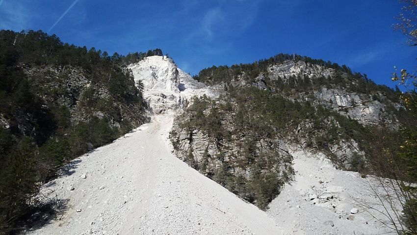
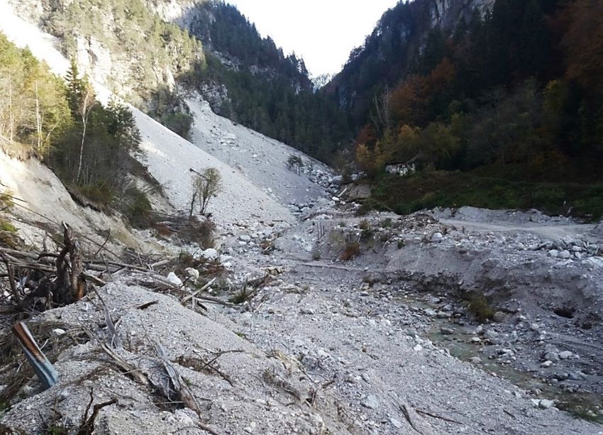
Tesi di Laurea Magistrale | Alessandro La Rocca, s244424

2. Site description
 The area of this study is in the North-West region of Slovenia, in Central Europe. It is
 located near the village of Belca in the municipality of Kranjska Gora, close to the
 Austrian border, about 60 km from Ljubljana, the capital city.

 Figure 2-1 – Geolocation of the site of interest.

 The site is mainly characterized by a fractured rock mass on the slope of a mountain, at the
 bottom of which the fallen debris has deposited (Figure 2-2a). The valley is short and narrow
 and it is crossed by a small torrent (Figure 2-2b) which flows into the Sava main river. Most
 of the bigger blocks accumlated in the years are on the upper portion of the torrent (Figure
 2-2c).

 From a geological point of view, the slope is made of Upper Triassic rocks, mainly light
 grey massive dolomite and layers of limstone, strongly tectonized.

 The slope has been monitored because a rock fall with a volume of 5000-10000 m3 occurred
 in September 2014. In the period from 2014 to 2017, both geotechincal and geological data
 were aquired by Lazar et al. [18]: in particular wire extensometers, tachometry, TLS and
 ALS were adopted.

POLITECNICO DI TORINO | Anno Accademico 2019/2020 12
Tesi di Laurea Magistrale | Alessandro La Rocca, s244424

 (a)

 (b) (c)

Figure 2-2 – Photographs of the site, taken during the last survey (October 24 th 2019): (a) the slope characterized
by the fractured rock mass and debris deposit, (b) the torrent along the valley and (c) the blocks accumulated over
the upper portion of the torrent.

 POLITECNICO DI TORINO | Anno Accademico 2019/2020 13
Tesi di Laurea Magistrale | Alessandro La Rocca, s244424

3. Data Acquisition
 The data for this study comes from seven different surveys, five of which were performed
 by members of University Ljubljana, Faculty of Civil and Geodetic Engineering (Fakulteta
 za gradbeništvo in geodezijo, FGG) and the remaining two were perform by the Department
 of Forestry and Renewable Forest Resources of the Biotechnical Faculty (Biotehinška
 Fakulteta, BF). They go from July 2018 to October 2019.

 The observed area changed in the first surveys: at first only the upper part was captured, then
 the entire riverbed has been once observed in order to detect the eventual transportation of
 the detached material and progressively only the portion of the river closer to the slope was
 sometimes considered in the survey.

 Figure 3-1 – DJI Mavic Air. (Figure from Figure 3-2 – DJI Phantom 4. (Figure from
 https://www.drone-store.it/prodotto/dji- https://www.amazon.it/DJI-PHANTOM-PRO-
 mavic-air-bianco/) OBSIDIAN-Risoluzione/dp/B075FVB86M)

 The data from BF were acquired with a DJI Mavic Air drone with a FC2103 camera model,
 having a focal length of 4.5 mm and returning images with a resolution of 4056x3040 pixels.
 No description of the surveys is given. Apparently, the flights weren’t performed
 systematically but by manual piloting of the drone.

 The data from FGG were acquired with a DJI Phantom 4 with a FC6310 camera model,
 having a focal length of 8.8 mm and images with a resolution of 5472x3648 pixels.
 The flight plans changed from a survey to another, learning from previous experiences (look
 at Table 3-1). At first only one flight for both the slope and the river was planned. Due to
 the complex geomorphology of the slope, 3 flights were planned with an oblique orientation
 of the camera (45°): the first two (fake and flat1) were performed at the same height, one
 having as reference a previous DTM of the area and the other one having as reference a plane
 with an inclination close to the overall slope; the third flight (flat 2) was performed as the
 second one but with a greater flying altitude in order to guarantee a greater overlap of the
 images. Then, the presence of isolated blocks and niches led to consider a different point
 view, so a flight with the camera orientated to the vertical direction was introduced. The
 portion of the river not close to the slope was no more considered and only one flight with
 an oblique camera was necessary to reduce the number of holes in the final model.

POLITECNICO DI TORINO | Anno Accademico 2019/2020 14
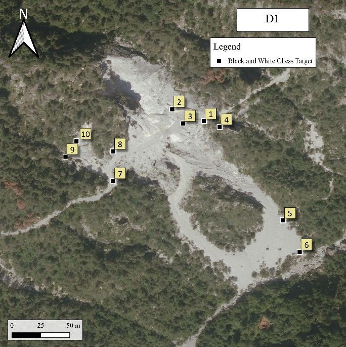
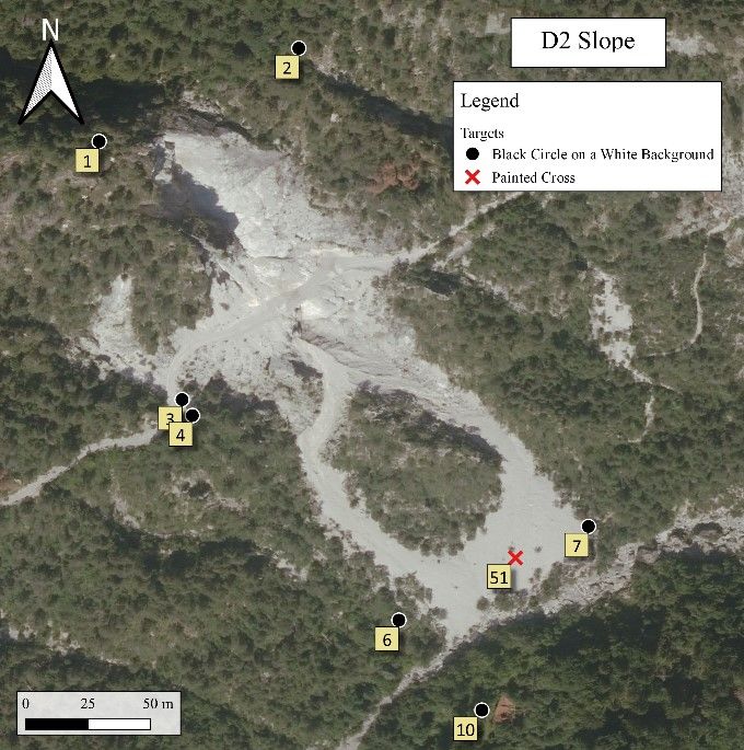
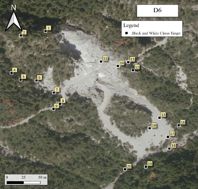
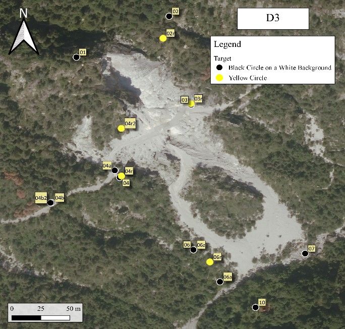
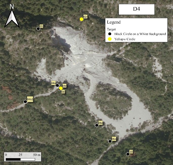
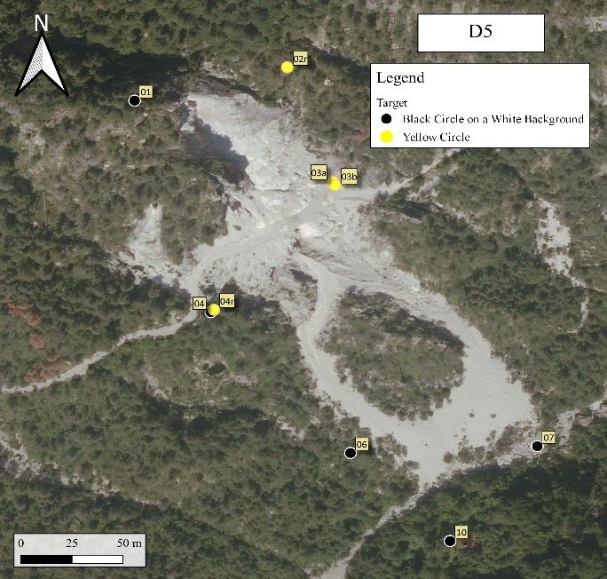
Tesi di Laurea Magistrale | Alessandro La Rocca, s244424

 Number Flying Ground Coverage Number
 Performed Flight’s
 Date of Orientation altitude resolution area of
 by Tag
 images (m) (cm/pix) (km2) targets
 D1 08-11-18 BF 110 / 122 3,69 10
 Slope 212 Oblique 63,6 1,6 0,0694 7
 D2 03-07-18 FGG
 Riverbed 133 Vertical 76,1 1,91 0,132 11
 Fake 159 Oblique 61,6 1,53 0,0524
 Flat 1 159 Oblique 62,9 1,6 0,0564 15
 D3 04-12-18 FGG
 Flat 2 159 Oblique 67,6 1,84 0.0186
 Riverbed 60 Vertical 81,2 2,24 0,00794 3
 Vertical 218 Vertical 92,6 2,53 0,0383
 D4 11-12-18 FGG Flat 246 Oblique 70,5 1,93 0,0305 18
 Fake 194 Oblique 68 1,86 0,0296
 Vertical 219 Vertical 90,2 2,46 0,0398
 D5 12-04-19 FGG 9
 Fake 166 Oblique 67,4 1,84 0,0258
 D6 18-10-19 BF 694 / 86,6 2,93 0,107 20
 Vertical 186 Vertical 96,2 2,62 0,04
 D7 24-10-19 FGG 8
 Fake 149 Oblique 90 2,46 0,0268

 Table 3-1 – Short description of the data

 In order to perform the georeferencing of the final model, the actual position of some control
 points was measured.

 Different kinds of targets for signalizing the ground control points have been used in the
 surveys. The BF adopted mainly chess-like black and white aerial targets (a), the only
 exception was for a marker in their second survey (D6) for which a cross was painted (d) on
 a rock. The FGG instead adopted two kinds of target: black circle on white frame (b) for
 those points on a horizontal plane and a yellow circle (c) for those points on a vertical plane
 (usually a rock wall or a tree). Also in this case, a green cross was painted on a block as a
 target.
 The actual measurements of the position of the targets were performed according to different
 geodetic methods.

 The methodology adopted by BF is unknown, but the coordinates available come with a
 level of accuracy between 1,5 and 4 cm both in horizontal and vertical direction.

 (a) (b) (c) (d)
 Figure 3-1 – Targets used in the surveys

POLITECNICO DI TORINO | Anno Accademico 2019/2020 15
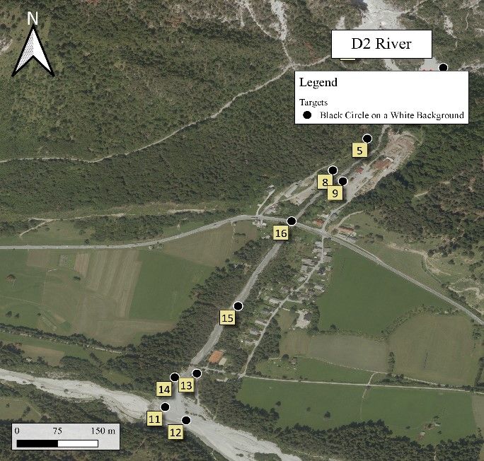
Tesi di Laurea Magistrale | Alessandro La Rocca, s244424

 The FGG adopted at first the methodology of RTK (Real-Time Kinematics) GNSS (Global
 navigation Satellite System) with an achieved accuracy of 0.04/0.08: due to problems with
 the GNSS signal some measurements came with a great error, so this method revealed to be
 not the optimum one. Later a combination of tacheometry and GNSS, with an accuracy in a
 rank of 2-3 cm, was adopted. Some of the instruments adopted in the survey of October 24th
 (D7) can be seen in Figures 3-4 (a)-(c).

 (a) (b) (c)

Figure 3-2 – Instruments for the topographic survey of October 24th (D7): (a) prism target on a tripod, (b) detail of
the prism target, (c) total station on a tripod.

 The number and the distribution of the target changed between the surveys. The main limit
 is instability of the slope and its accessibility. Some targets were placed out of the body of
 the rockslide: at the top, at the bottom, and some on the sides of the main body, thanks to the
 presence of a road that used to go through the slope before being covered by the debris flow.

 Every target used for each survey is shown in the following figures (Figures 3-6). Not all of
 them were used as GCP (Ground Control Points) or CP (Check Point) because sometimes
 the difference between the estimated position and the input coordinates was too big
 (probably due to some errors in the acquisition of the spatial datum) or the number of
 projections (how many times the target appears into the images) were lower than 2.

POLITECNICO DI TORINO | Anno Accademico 2019/2020 16
Tesi di Laurea Magistrale | Alessandro La Rocca, s244424

 Figure 3-5 – Targets adopted during the photogrammetric surveys.

POLITECNICO DI TORINO | Anno Accademico 2019/2020 17
Tesi di Laurea Magistrale | Alessandro La Rocca, s244424

4. Data processing
 Photogrammetry is a discipline that allow to build a 3D model of an object or the terrain
 starting from the acquisition of many images from different points of view. A valid
 reconstruction of a geometry, in terms of dimension and shape, depends on the accurate
 estimation of the interior and exterior orientation of the cameras: they define the actual inside
 geometry of the camera and its position and rotation for every photo taken.

 In order to perform such procedure, the software Agisoft Metashape Pro (version 1.5) has
 been used. It uses a Structure from Motion (SfM) that allows the matching of the features of
 many images in order to reconstruct the camera motion and the geometry of a 3D scene. This
 process, after some elaborations, lead to a georeferenced dense point cloud that can later be
 imported into the software CloudCompare (version 2.6.1) for multi-temporal change
 detection by meaning of point cloud comparison.

 The general workflow adopted follows these steps:

 1. Import and alignment of the images
 2. Input of GCP coordinates
 3. Cleaning sparse point cloud by gradual selection Agisoft Metashape
 4. Optimization of the georeferencing
 5. Building of dense point cloud
 6. Classification

 7. Noise filtering
 8. Registration Cloud Compare
 9. Estimation of cloud-to-cloud distance
 10. Calculation of volume changes

 These procedures were carried out with the following system configuration (Table 4-1).

 Processor Intel® Core™ i7-9700 CPU @ 3.00GHz 3.00GHz
 RAM 64 GB
 System type 64-bit Operating System, x64-based processor
 Graphic Card NVIDIA GeForce GTX 1660
 Table 4-1 – System configuration.

POLITECNICO DI TORINO | Anno Accademico 2019/2020 18
Tesi di Laurea Magistrale | Alessandro La Rocca, s244424

4.1. Import and alignment of the images
 The first step was to load the photos into the software. In case of multiple flights in a single
 survey, multiple sets of photos were available: these were loaded in different chunks in order
 to have one single project for every flight.

 In order to obtain a first three-dimensional reconstruction of the area, the photos must be
 aligned. The software looks for characteristic points in every image, the so-called Key
 Points, and tries to match them in order to define the Tie Points. A limit for both key points
 and ties points, can be defined by the operator according to his necessities: in this case the
 default parameters was adopted (respectively 4’000 and 30’000).

 Figure 4-1 Example of image-matching of feature points: the blue lines stand for a valid matching, the
 purple one stand for an invalid matching.

 During this process, the collinearity equations are solved and the camera motion is
 reconstructed by the estimation the camera locations. The accuracy of this process can be
 defined by the operator: medium, low and lowest setting cause image downscaling
 respectively by a factor of 4, 16 and 64; the highest accuracy setting, instead, upscales the
 images by a factor of 4 allowing a better estimation of the tie points location. Since this
 choice strongly affects the time of the processing, the default high accuracy setting was
 adopted and the software worked with the original size of the images (Agisoft Metashape
 user manual [2]).

 The images come along with the camera position and rotation measured by the drone itself
 in a WGS84 (EPSG 4326) coordinate system, so they were used to perform a preliminary
 pair selection of the photos. It is also possible to perform a generic preselection of the
 overlapping photos by matching them using lower accuracy setting first. In order to reduce
 the time of processing, both reference and generic preselection were performed.

 At this point, a sparse cloud of points is generated. The results of the alignment can be seen
 Figure 4-2 (a)-(g). (Must be noted that the shown result come from merging the different
 chunks for every survey and this step is based on the markers that will be introduced only in
 the following steps). Most of the points, excluding the model D2, occur on more than 9
 photos.

POLITECNICO DI TORINO | Anno Accademico 2019/2020 19
Tesi di Laurea Magistrale | Alessandro La Rocca, s244424

 D1 D2 - Slope

 D2 - River D3

 D4 D5

POLITECNICO DI TORINO | Anno Accademico 2019/2020 20
Tesi di Laurea Magistrale | Alessandro La Rocca, s244424

 D6 D7

 Figure 4-2 - Camera location and overlap of the images

4.2. Input of GCP coordinates
 A three-dimensional model generated by aerial images by using an Unmanned Aerial
 Vehicles (UAV) can be used to perform accurate measurements only if it is properly
 registered in a specific coordinate system. In this way, the model can be easily loaded in
 geoviewers and geographic informative systems (GIS). There are two basic approaches to
 perform the georeferencing of the model: direct and indirect. The direct method is based on
 the presence of sensors that measures position (easting, northing and altitude) and orientation
 (yaw, pitch and roll) of the camera for every image (Reese et al. []). In this case, both the
 drones have a GPS (Global Positioning System) and GLONASS (GLObal NAvigation
 Satellite System) sensor installed. The indirect method is based on the access to the absolute
 position of some points in the interested area, with a level of accuracy accordingly to
 methodology adopted for the topographic survey. These points are called Ground Control
 Points (GCP), usually signalized with targets, and they can be introduced by inserting
 markers over the set of images: each marker is associated with one target visible and
 recognizable in a subset of images. The first solution is the cheaper and the less time-
 consuming, but it is very sensible to interference and it can be affected by vehicle
 malfunction or construction errors, so the estimated parameters may come with great
 uncertainties (Zhu et al. []). More accurate results can be achieved by meaning of the indirect
 georeferencing, even if it’s an expensive and time-consuming method. In addition to the time
 required for the geodetic survey, the right positioning of each marker is not immediate and
 it may require a critical judgment from the operator. After adding a marker in a single photo
 were the target is visible, Agisoft Metashape is able to automatically recognize its projection
 in the other photos but this process isn’t always precise, leading to different problem that
 requires the manual intervention:

 • the projected marker can be far away from the actual target;
 • even if the target is present, it can be not visible: it could be covered by the vegetation,
 abundant on the perimeter of the area of study were the target were placed, or it could

POLITECNICO DI TORINO | Anno Accademico 2019/2020 21
Tesi di Laurea Magistrale | Alessandro La Rocca, s244424

 be overexposed due to the sunlight accordingly to weather condition, time of the day
 and spatial orientation of the target itself;
 • low resolution of the target due to the distance of the camera: photographs taken over
 the middle portion of the area could contain the targets place at the bottom because of
 the steep inclination of the slope;
 • perspective deformation of the target: this makes difficult recognizing the center of the
 target and this happen in most cases with the yellow circle targets that were placed on a
 sub-vertical or vertical surface (rock-wall or a tree).

 If at first a number of projected markers in a range of 20-200 was found, after checking every
 singular photo it has been reduced to a number in the range of 5-30. The remaining markers
 were correctly placed in order to reduce the reprojection error in term of pixels, defined by
 the user manual [2] as “the distance between the point on the image where a reconstructed
 3D point can be projected and the original projection of that 3D point detected on the photo
 and used as a basis for the 3D point reconstruction procedure.” In particular, for each
 marker the error (pix) is equal to the root mean square reprojection error calculated over all
 the valid tie points recognized in the images. The goal was to obtain a reprojection error
 lower than 0.5-0.6 pixels.

 The points coordinates in terms of northing, easting and altitude in coordinate system of
 Slovenia 1996/Slovene National Grid (EPSG::3794) were then imported after correctly
 naming the label of each target: differently from a direct method of georeferencing, using
 GCPs requires a proper labeling of the measurements and an accurate scheme of the spatial
 distribution of the targets. The data from BF came with a value of accuracy for each GCP;
 the data from FGG didn’t have any accuracy value and at this stage the default value of 0.005
 m was applied. The later definition of this parameter is discussed in the chapter 4.4
 Optimizing georeferencing.

 By this process, the model is transformed by estimating 7 parameters (3 for translation, 3 for
 rotation and 1 for scaling) in order to obtain a valid reconstruction of the terrain, every point
 of which is associated to three spatial coordinates in a known reference system. This can
 also help to compensate the eventual linear errors in the first alignment of the cameras. Since
 the overlapping of the images and the shape of the terrain could lead also to non-linear
 deformation of the model, the camera alignment must be optimized. This is performed by
 the software thanks to an algorithm that minimizes the sum of reference coordinate
 misalignment error and reprojection error while adjusting the estimated point coordinates
 and the camera parameters. The operator can choose which camera parameter change in the
 optimization between:

 • f: focal length;
 • cx, cy: coordinates of the principal point;
 • b1, b2: affinity and skew transformation coefficients;
 • k1, k2, k3, k4: radial distortion coefficients;
 • p1, p2, p3, p4: tangential distortion coefficients.

POLITECNICO DI TORINO | Anno Accademico 2019/2020 22
Tesi di Laurea Magistrale | Alessandro La Rocca, s244424

 At this stage, the default options (f, cx, cy, k1, k2, k3, p1, p2) were good enough to appreciate
 a strong correction of camera alignment.

 Some markers showed greater value of error, indicating a possible outlier in the
 measurements. Before eventually remove these markers, the cleaning of the point cloud was
 performed in order to obtain better result from optimizing the cameras parameters in the
 following steps since this process is affected by the presence of mislocated points.

4.3. Cleaning the sparse point cloud by gradual selection
 A Structure form Motion software allows to build a 3D model from a series of images by
 finding feature points in every image and simultaneously estimating the internal and external
 camera parameters. This process can lead to both linear and non-linear errors in the
 reprojection of the terrain into the virtual environment. Georeferencing the model by
 introducing the measured spatial coordinates of GCps could compensate the linear error, but
 in order to correct the non-linear errors the optimization of camera parameters must be
 performed. This is a useful and powerful tool since it strongly affects the final result of the
 georeferencing. It is used every time after changing the GCPs in order to look for a possible
 outlier or selecting the proper set of CPs to verify the quality of the georeferencing. This is
 the reason why the sparse point cloud must be edited: the estimation of camera parameters
 and the quality of the reprojection depends on the presence of mislocated points.

 The selection of the points to remove is performed by setting a threshold for each of these
 parameters:

 • Reprojection error: it indicates a poor localization accuracy of corresponding point
 projections in the phase of point matching;
 • Reconstruction uncertainty: it indicates a strong deviation from the object surface,
 so it’s correlated to the noise in the point cloud (should not affect the accuracy of the
 optimization, but useful for a better visual appearance of the cloud);
 • Image count: it indicates the number of photos in which every point is visible, it’s
 directly proportional to location accuracy;
 • Projection accuracy: it indicates the accuracy in localizing the projections of the
 points due to their size.

 In order to find the best way to perform such selection, different approaches were considered
 in order to obtain a good reconstruction of the 3D model without losing too many points.

POLITECNICO DI TORINO | Anno Accademico 2019/2020 23
Tesi di Laurea Magistrale | Alessandro La Rocca, s244424

The approaches adopted and compared are:

 • CLEAN 0: this method is the simplest and it has based on an application in
 archeological and cultural heritage studies by Dr. Heinrich Mallison [20]. A value of
 80-90% of the maximum reprojection error was set as a threshold: points with greater
 error were removed. In case of reconstruction uncertainty and projection error, a
 threshold of 10 was set. After the removal of the points ended, the optimization of the
 cameras has been run with the default parameters selected. Due to the different kind of
 field of application, new approaches were tested.
 • CLEAN 1A: this method introduced the principle of setting the threshold value in order
 to obtain the selection of 5-10% of the points of the sparse cloud, since the previous
 approached sometimes led to a very small or very large selection of points. The
 sequence of the parameters adopted in the gradual selection and the default options in
 optimizing the cameras were kept unchanged.
 • CLEAN 1B: this approach mixes the methods CLEAN 1A and CLEAN 2. The order of
 the parameters used in the gradual selection and the 5-10% threshold principle were
 kept unchanged. After removing the selected points, the camera parameters were
 optimized each time: in case of reconstruction uncertainty and projection accuracy, all
 the parameters of the camera were considered.
 • CLEAN 2: this method is based on the introductory training class in Unmanned Aircraft
 Systems Data Post-Processing proposed by United States Geological Survey (USGS)
 [32], the sole science agency for the Department of the Interior of the United States of
 America. This is the most complex method adopted, but it finds its application in the
 reconstruction of a terrain model from aerial surveys so it closer to this study. The
 sequence of the parameters used in the gradual selection changed and after removing
 the selected points the optimization of cameras was perform selecting all the camera
 parameters for the selections based on the projection accuracy and reprojection error.
 The selections based on the reconstruction uncertainty and projection accuracy were run
 twice. Also in this case the 5-10% threshold principle was adopted.

 The image count wasn’t considered in any of the methods and for any of the data sets, since
 setting a threshold number immediately lower then given value (3) would have selected a very
 large number of points, close to 50%. This process would have removed those points that are
 present only in 2 images but in these cases it would have strongly affected the characterization
 of the slope and the quality of the final model.

 The parameters adopted for each data set is shown in Table 4-2.

 In order to reduce the time of the cleaning process, for every survey the sparse point cloud
 generated from the different flights were merged into one single point cloud. This step was
 performed based on the position of the markers. A previous alignment of the models wasn’t
 performed since the presence of the vegetation and holes in the model due to the complex
 geomorphology of the site would have led to bad results. Merging the point clouds wasn’t
 accurate in one particular case, as it can be seen in the 5th chapter about the comparison of
 the models.

POLITECNICO DI TORINO | Anno Accademico 2019/2020 24
You can also read