Quantifying iceberg calving fluxes with underwater noise - The Cryosphere
←
→
Page content transcription
If your browser does not render page correctly, please read the page content below
The Cryosphere, 14, 1025–1042, 2020
https://doi.org/10.5194/tc-14-1025-2020
© Author(s) 2020. This work is distributed under
the Creative Commons Attribution 4.0 License.

Quantifying iceberg calving fluxes with underwater noise
Oskar Glowacki1,2 and Grant B. Deane1
1 Marine   Physical Laboratory, Scripps Institution of Oceanography, La Jolla, California, USA
2 Institute of Geophysics, Polish Academy of Sciences, Warsaw, Poland

Correspondence: Oskar Glowacki (oglowacki@ucsd.edu)

Received: 18 October 2019 – Discussion started: 4 November 2019
Revised: 5 February 2020 – Accepted: 13 February 2020 – Published: 17 March 2020

Abstract. Accurate estimates of calving fluxes are essential      1     Introduction
in understanding small-scale glacier dynamics and quantify-
ing the contribution of marine-terminating glaciers to both       1.1    The role of iceberg calving in glacier retreat and
eustatic sea-level rise (SLR) and the freshwater budget of               sea-level rise
polar regions. Here we investigate the application of acousti-
cal oceanography to measure calving flux using the underwa-
ter sounds of iceberg–water impact. A combination of time-        The contribution of glaciers and ice sheets to the eustatic
lapse photography and passive acoustics is used to determine      sea-level rise (SLR) between 2003 and 2008 has been esti-
the relationship between the mass and impact noise of 169         mated to be 1.51 ± 0.16 mm of sea-level equivalent per year
icebergs generated by subaerial calving events from Hans-         (Gardner et al., 2013). Cryogenic freshwater sources were
breen, Svalbard. The analysis includes three major factors af-    responsible for approximately 61 ± 19 % of the total SLR
fecting the observed noise: (1) time dependency of the ther-      observed in the same period. Iceberg calving, defined as me-
mohaline structure, (2) variability in the ocean depth along      chanical loss of ice from the edges of glaciers and ice shelves
the waveguide and (3) reflection of impact noise from the         (Benn et al., 2007), is thought to be one of the most im-
glacier terminus. A correlation of 0.76 is found between the      portant components of the total ice loss. For example, solid
(log-transformed) kinetic energy of the falling iceberg and       ice discharge accounts for around 32 % to 40 % of the mass
the corresponding measured acoustic energy corrected for          loss from the Greenland ice sheet (Enderlin et al., 2014;
these three factors. An error-in-variables linear regression is   van den Broeke et al., 2016), and iceberg calving in Patag-
applied to estimate the coefficients of this relationship. En-    onia dominates glacial retreat (Schaefer et al., 2015). On
ergy conversion coefficients for non-transformed variables        the other hand, several studies found that increased subma-
are 8×10⁻⁷ and 0.92, respectively, for the multiplication fac-    rine melting is a major factor responsible for the observed
tor and exponent of the power law. This simple model can be       rapid retreat of tidewater glaciers (e.g., Straneo and Heim-
used to measure solid ice discharge from Hansbreen. Uncer-        bach, 2013; Luckman et al., 2015; Holmes et al., 2019). The
tainty in the estimate is a function of the number of calv-       exact partitioning between ice mass loss caused by calving
ing events observed; 50 % uncertainty is expected for eight       fluxes, submarine melting and surface runoff changes geo-
blocks dropping to 20 % and 10 %, respectively, for 40 and        graphically and needs to be measured separately at each lo-
135 calving events. It may be possible to lower these errors if   cation. Calving from tidewater glaciers is driven by differ-
the influence of different calving styles on the received noise   ent mechanisms, including buoyant instability, longitudinal
spectra can be determined.                                        stretching and terminus undercutting (van der Veen, 2002;
                                                                  Benn et al., 2007). Terminus undercutting results from sub-
                                                                  marine melting and is often considered to be a major trigger
                                                                  of ice breakup at the glacier front (Bartholomaus et al., 2013;
                                                                  O’Leary and Christoffersen, 2013). In support of this idea,
                                                                  the solid ice discharge from tidewater glaciers was found
                                                                  to be highly correlated with ocean temperatures (P˛etlicki

Published by Copernicus Publications on behalf of the European Geosciences Union.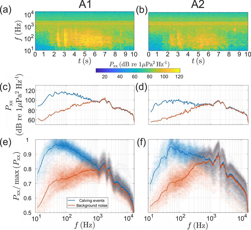
1026                              O. Glowacki and G. B. Deane: Quantifying iceberg calving fluxes with underwater noise

et al., 2015; Luckman et al., 2015; Holmes et al., 2019),           Yahtse Glacier, Alaska, with estimates of iceberg sizes di-
which are expected to increase significantly as a result of cli-    vided into seven classes. In line with previous findings by
mate shifts (IPCC, 2013). Thus, accurate estimates of calving       Qamar (1988), they identified ice quake duration as the most
fluxes from marine-terminating glaciers are crucial to both         significant predictor of iceberg volume. Based on these stud-
understanding glacier dynamics and predicting their future          ies, Köhler et al. (2016, 2019) successfully reconstructed a
contribution to SLR and the freshwater budget of the po-            record of total frontal ablation at Kronebreen, Svalbard, us-
lar seas. Obtaining these estimates requires remote-sensing         ing seismic data calibrated with satellite images and lidar
techniques, which enable the observation of dynamic glacial         volume measurements.
processes from a safe distance.                                        Recently, Minowa et al. (2018, 2019) demonstrated the
   Satellite imagery is an effective way to study large-scale,      potential of using surface waves generated by falling ice-
relatively slow changes at the ice–ocean interface, such as         bergs to quantify calving flux. They found a strong corre-
the disintegration of the 15 km long ice tongue from Jakob-         lation between calving volumes estimated from time-lapse
shavn Isbræ in 2003 in Greenland (Joughin et al., 2004).            camera images and the maximum amplitudes of the waves.
For fast-flowing ice masses, changes of terminus position           Other methods for quantifying ice discharge from marine-
caused by both calving and glacier flow must be clearly sepa-       terminating glaciers, including surface photography (e.g.,
rated. Consequently, satellite imagery is more limited for ob-      How et al., 2019), terrestrial laser scanning (e.g., P˛etlicki and
serving calving events, which typically occur on sub-diurnal        Kinnard, 2016), ground-based radar imaging (e.g., Chapuis
timescales and are often not greater than 1000 m3 in volume         et al., 2010) or terrestrial radar interferometry (e.g., Walter et
for most tidewater glaciers in Svalbard or Alaska (e.g., Cha-       al., 2019), are usually used for short-term measurements.
puis and Tetzlaff, 2014). Moreover, a thick layer of clouds,
fog or precipitation in the form of snow and rain often makes       1.3   Studying iceberg calving with underwater noise
it difficult to track iceberg calving continuously using op-
tical techniques, such as surface photography or terrestrial        The approach investigated here is an example of acousti-
laser scanning. These difficulties provide the motivation for       cal oceanography, which extracts environmental information
investigating the use of underwater noise to quantify calving       from the underwater noise field (Clay and Medwin, 1977).
fluxes.                                                             Acoustical oceanography may offer some advantages over
                                                                    other, more well-developed methods for the study of the
1.2    Measuring ice discharge – tools and methods                  interactions between land-based ice and the ocean. Low-
                                                                    cost hydrophones are easily deployed in front of marine-
Many different methods have been developed to mea-                  terminating glaciers, and acoustic data can be gathered con-
sure ice discharge from marine-terminating glaciers. Passive        tinuously for several months or longer with a high (>
glacier seismology, also called “cryoseismology” (Podol-            10 000 Hz) sampling rate and low maintenance. Measure-
skiy and Walter, 2016), is probably one of the most mature,         ments are insensitive to lighting conditions such as fog; cloud
widespread and useful tools; broadband seismometers have            coverage; and the polar night, humidity and intensity of
been widely installed in remote areas near calving glaciers         precipitation. Moreover, acoustic signals recorded in glacial
since the early studies performed by Hatherton and Evison           bays and fjords also contain signatures of ice melt associated
(1962) and Qamar and St. Lawrence (1983). Seismic signals           with impulsive bubble release events (Urick, 1971; Tegowski
associated with subaerial calving originate from two main           et al., 2011; Deane et al., 2014; Pettit et al., 2015; Glowacki
mechanisms: (1) the free fall of ice blocks onto the sea sur-       et al., 2018). While currently no quantitative models exist to
face (Bartholomaus et al., 2012) and (2) interactions between       estimate melt rates from underwater noise, the potential idea
detaching icebergs and their glacier terminus (e.g., Ekström        to simultaneously measure submarine melting and calving,
et al., 2003; Murray et al., 2015). The latter interactions, also   two major processes acting at the glacier–ocean interface, is
known as “glacial earthquakes”, are caused by large, cubic-         worth mentioning.
kilometer-scale icebergs of full-glacier height, and the result-       Quantifying iceberg calving by “listening to glaciers”
ing seismic magnitude is not related to the iceberg volume          was first proposed by Schulz et al. (2008), who suggested
in a simple manner (Sergeant et al., 2016). Higher-frequency        long-term deployments of hydrophones (underwater micro-
(> 1 Hz) calving seismicity from iceberg–ocean interactions,        phones) and pressure gauges, in addition to more traditional
constantly detected by distant seismic networks (e.g., O’Neel       measurements of water temperature and salinity, to study
et al., 2010; Köhler et al., 2015), usually peaks between 1         signals of ice discharge together with accompanying hydro-
and 10 Hz (Bartholomaus et al., 2015; Köhler et al., 2015).         graphic and wave conditions. Following this novel idea, in-
Both frequency content and amplitudes of high-frequency             dependent studies conducted in Svalbard (Tegowski et al.,
signatures are found to be independent of iceberg volumes           2012) and Alaska (Pettit, 2012) showed the first waveforms
(O’Neel and Pfeffer, 2007; Walter et al., 2012). Bartholo-          and spectra of the sounds generated by impacting ice blocks.
maus et al. (2015) applied generalized linear models to cor-        Pettit (2012) provided an explanation for individual com-
relate various properties of seismic signals originating at         ponents of the signal, including low-frequency onset, pre-

The Cryosphere, 14, 1025–1042, 2020                                                      www.the-cryosphere.net/14/1025/2020/
O. Glowacki and G. B. Deane: Quantifying iceberg calving fluxes with underwater noise                                          1027

calving activity, mid-frequency block impact, iceberg os-
cillations, and mini-tsunami and seiche action. Encouraged
by these initial results, Glowacki et al. (2015) analyzed 10
subaerial and 2 submarine calving events identified in both
acoustic recordings and time-lapse photography made in
front of Hansbreen, Svalbard. A spectral analysis of three
different calving types, called “typical subaerial”, “sliding
subaerial” and “submarine” (see supplementary videos in
Glowacki et al., 2015), showed that they radiated underwater
noise in distinct spectral and temporal patterns, but all with
a spectral peak between 10 and 200 Hz. Most importantly,
acoustic emission below 200 Hz was highly correlated with
block impact energy in a simple model. The dimensionless
coefficient converting impact energy to acoustic energy at the
calving impact point was found to be 5.16 × 10⁻¹⁰ , and the
power exponent was assumed to be 1. However, this earlier
analysis was limited by the small number of subaerial calv-
ing events analyzed (10), lack of a full error analysis and
the unrealistic assumption of simple cylindrical spreading of     Figure 1. A map of the study site (a) and representative cropped
                                                                  time-lapse image taken by Cam 1 (b). (a) Locations of time-
acoustic waves in the water column.
                                                                  lapse cameras, acoustic buoys, calving events and CTD casts are
   To address these issues, we conducted a new study cov-         marked with white, black, yellow and red dots, respectively. Col-
ering a total number of 169 subaerial calving events ob-          ored, dashed lines show transects of CTD surveys oriented per-
served with time-lapse photography at Hansbreen, Svalbard.        pendicular (red) and parallel (blue) to the glacier terminus. Black
Impact energies generated by falling icebergs are estimated       dashed lines show the spatial arrangement of bathymetry profiles,
with error bars and related to received acoustic signals. The     which we used to model noise transmission losses. Landsat 8 satel-
total noise energy resulting from block–water impact is cal-      lite data collected on 27 August 2016, courtesy of the US Geo-
culated using a standard sound propagation model Bellhop          logical Survey, Department of the Interior. Bathymetric data pro-
(Porter, 1987, 2011), which requires bathymetry data and          vided by the Norwegian Hydrographic Service under the permit no.
sound speed profiles as inputs. Variability in transmission       13/G722, issued by the Institute of Geophysics, Polish Academy of
losses associated with sound wave reflections from an ideal-      Sciences.
ized, flat glacier terminus is also accounted for. The analysis
shows that impact energy is strongly correlated with acoustic
emission below 100 Hz. We present a new energy conversion
efficiency calculated with this more detailed physical model      tively (Błaszczyk et al., 2009). The average retreat rate of the
and demonstrate how cumulative values of kinetic energy and       glacier during 2005–2010, 44 m yr−1 , was more than twice
ice mass loss can be found by integrating impact noise over       the rate observed between 1900 and 2010 (Grabiec et al.,
a specified number of subaerial calving events.                   2012). These characteristics are representative of Svalbard’s
                                                                  tidewater glaciers, making the bay of Hansbreen a good study
                                                                  site.
2     Study area                                                     Both glacial behavior and the propagation of sound are
                                                                  sensitive to temporal variability in thermohaline structure of
2.1    General setting                                            water masses in the bay (P˛etlicki et al., 2015; Glowacki et
                                                                  al., 2016). The calving activity of Hansbreen is largely con-
Hansbreen is a retreating, grounded, polythermal tidewater        trolled by melt-driven undercutting of the ice cliff (P˛etlicki et
glacier terminating in Hornsund fjord, Svalbard (Fig. 1). It      al., 2015). The water temperature and salinity in the center of
covers an area of around 54 km2 and is more than 15 km            the bay ranged from −1.8 ◦ C to more than 2.0 ◦ C and from
long (Błaszczyk et al., 2013). The glacier has a 1.5 km-          30 PSU to almost 35 PSU during 2015 and 2016 (Moskalik et
wide active calving front with an average height of around        al., 2018). Significant wave height observed in the study site
30 m (Błaszczyk et ’al., 2009). The mean thickness and to-        reached a maximum value of around 1.5 m over the period of
tal volume of Hansbreen are estimated to be 171 m and             August–November 2015 (Herman et al., 2019). A geomor-
9.6 ± 0.1 km3 , respectively (Grabiec et al., 2012). The sur-     phological map of the bay reveals complicated structures in
face flow of the glacier is dominated by basal motion in          the seabed created by dynamic glacial processes acting after
the ablation area (Vieli et al., 2004) and the mean annual        the Little Ice Age, including terminal moraines, flat areas and
flow velocity near the terminus, and its calving flux is es-      iceberg-generated pits, to name a few (Ćwiakała
                                                                                                               ˛     et al., 2018).
timated to be 150 m yr−1 and 38.1 × 10⁶ m3 yr−1 , respec-         The water depth along a transect parallel to the glacier termi-

www.the-cryosphere.net/14/1025/2020/                                                     The Cryosphere, 14, 1025–1042, 2020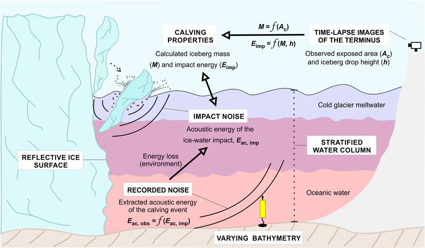
1028                                O. Glowacki and G. B. Deane: Quantifying iceberg calving fluxes with underwater noise

                                                                       Figure 3. Bathymetry profiles between the terminus of Hansbreen
                                                                       and the two acoustic buoys: A1 (a) and A2 (b). The spatial arrange-
                                                                       ment of the transects, which are numbered clockwise, is shown
                                                                       in Fig. 1. The horizontal axis is zeroed at locations of the buoys,
                                                                       marked with black dots. Bathymetric data provided by the Norwe-
                                                                       gian Hydrographic Service under the permit no. 13/G722, issued by
Figure 2. (a–d) Sound velocity profiles for CTD surveys oriented       the Institute of Geophysics, Polish Academy of Sciences.
perpendicular (red) and parallel (blue) to the glacier terminus, to-
gether with (e) the corresponding frequency of calving occurrence.
Locations of the CTD transects taken during the study period are       the study period. Moreover, significant differences in sound
shown in Fig. 1 with the same red and blue colors. Thick, dashed       velocity profiles taken on the same day were also observed
lines mark the dates of the CTD measurements. Blue numbers in          between different locations perpendicular and parallel to the
the lower panel (e) provide the number of calving events assigned      glacier terminus, driven by a complex and three-dimensional
to each set of sound speed profiles.                                   distribution of the thermohaline field in the bay. The ocean
                                                                       depth between the locations of calving events and the two
                                                                       acoustic buoys varied from 10 m on underwater sills to more
nus ranges from less than 20 to almost 90 m (see Fig. 5 in             than 80 m in the western part of the bay near the terminus
Moskalik et al., 2018).                                                (Fig. 3). The bathymetry profiles were very different for the
                                                                       two buoy locations, with a more variable depth observed in
2.2    Calving activity and sound propagation conditions               the case of the buoy deployed further from the glacier cliff.

The main dataset consists of more than a thousand subaerial
calving events observed between 30 July and 15 Septem-                 3   Methods and data analysis
ber 2016, with three time-lapse cameras and two acoustic
buoys deployed in the glacial bay (Fig. 1). At least 20 ice            The development of underwater acoustics as a new tool for
blocks calved each day. It was not always possible to un-              quantifying calving fluxes requires thorough understanding
ambiguously identify a calving event in both the image and             of the causal relationship between the energy of the ice–
acoustic datasets; the occurrence of more than one iceberg             water interaction and the resulting noise emission. In this
detachment between the two consecutive images resulted in              section we discuss all steps that are necessary to complete
ambiguity in the acoustic data. Moreover, dense fog, rain or           this task. They are illustrated in Fig. 4 and described in detail
otherwise unfavorable lighting conditions would at times ob-           in the following subsections. Firstly, a time-lapse camera is
scure the terminus. From the total calving inventory, a sub-           used to estimate iceberg dimensions and block impact ener-
set of N = 169 events were unambiguously matched and                   gies (Sect. 3.1). Secondly, an underwater noise from iceberg–
analyzed (Figs. 1 and 2). The observer present in the field            water impact is recorded at a safe distance from the glacier
throughout the data collection phase reported that no anthro-          terminus and analyzed to find its amplitude–frequency char-
pogenic sound sources were active during the occurrence of             acteristics (Sect. 3.2). Then, in order to calculate impact
these calving events.                                                  noise energy at source, two factors have to be considered:
   Measurements of ocean temperature and salinity in the bay           (1) transmission loss in a waveguide, which depends on the
revealed upward-refracting sound speed profiles, with veloci-          distance to the buoy, sea bottom properties along the propa-
ties changing from around 1440 m s−1 just below the surface            gation path and variable thermohaline conditions (Sect. 3.3
to almost 1470 m s−1 close to the bottom (Fig. 2a–d). The              and 3.4.1), and (2) the potential contribution of acoustic en-
sound speed gradient between the surface layer and deeper              ergy reflected from the underwater part of the glacier termi-
layers, which controls refraction and transmission loss, is            nus on the received calving noise (Sect. 3.4.2). Finally, a sim-
driven by fresh meltwater and was clearly increasing during            ple model relating impact noise energy to the kinetic energy

The Cryosphere, 14, 1025–1042, 2020                                                         www.the-cryosphere.net/14/1025/2020/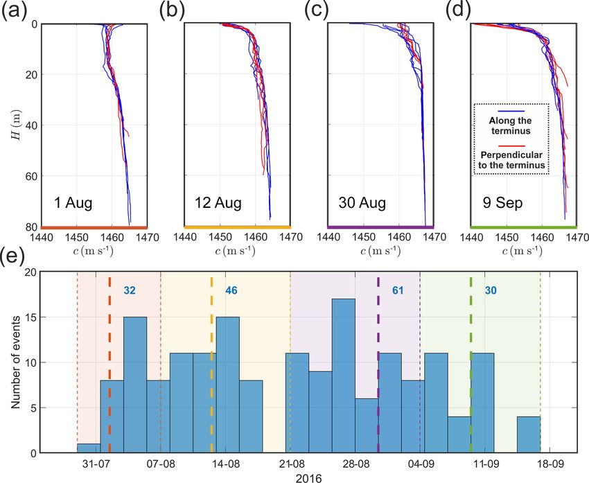
O. Glowacki and G. B. Deane: Quantifying iceberg calving fluxes with underwater noise                                        1029

of the falling ice block is proposed (Sect. 3.5). The param-       energy of the impacting ice block, Eimp , is given by
eters of this model are derived and investigated further in
Sect. 4 to demonstrate a new method for quantifying calv-          Eimp = Mgh = V ρi gh,                                       (3)
ing fluxes from underwater noise recordings.
                                                                   where ρi is the ice density, set to be a constant 917 kg m−3 ,
3.1    Photographic observation of calving events                  g = 9.81 m s−2 is the acceleration due to gravity and M is the
                                                                   iceberg mass. Equation (3) for Eimp is based on the assump-
Images of the Hansbreen terminus were taken every 15 min           tion that there is no energy dissipated during the free fall
from three locations (“Cam 1–3” in Fig. 1) continuously            of an iceberg. In reality, energy is dissipated though various
between 30 July and 15 September 2016 using Canon                  physical mechanisms, such as friction between an ice block
EOS 1100D cameras (4272 pixel×2848 pixel resolution and            and glacier terminus, momentum transfer at the early stage of
18 mm focal length). The three cameras were not perfectly          the water entry, drag during the immersion phase, and block
synchronized, which in fact enabled better separation of in-       disintegration, which can happen at different stages of calv-
dividual iceberg calving events occurring shortly after one        ing. However, the details of these hydrodynamic processes
other. Additionally, a GoPro Hero 3+ camera was placed             lie beyond the scope of this work. Because they are not in-
closer to the terminus to take pictures of the narrow ice cliff    cluded, Eq. (3) provides an upper bound of the total amount
segment (“GoPro” in Fig. 1). This camera took images at a          of energy available for noise production during the block–
much higher rate of 1 s−1 but was not always active during         water interaction.
the deployment. Iceberg volume and drop height were esti-
mated using images from Cam 1, which had the most perpen-          3.2   Impact noise recordings and analysis
dicular orientation to the glacier front of all the cameras. The
                                                                   The acoustic data were recorded continuously between
irregular shape of the ice cliff provided registration features,
                                                                   30 July and 15 September 2016 using two HTI-96-MIN
which were identified in both Landsat 8 satellite images (with
                                                                   omnidirectional hydrophones deployed at depths of 40 and
resolution of 15 m) and the camera images, enabling a precise
                                                                   22 m, respectively, in front of Hansbreen (“A1” and “A2” in
localization of calving events.
                                                                   Fig. 1). The hydrophones have a sensitivity of −164 dB re
    Following Minowa et al. (2018), the volumes of the calved
                                                                   1 V µPa−1 and were sampled at a rate of 32 kHz at a resolu-
ice blocks are estimated from the area at the glacier terminus
                                                                   tion of 16 bit. A single mooring system consisted of an an-
exposed by the calving event. Newly exposed areas are iden-
                                                                   chor, short line and acoustic buoy with a hydrophone, pow-
tified from differences between pairs of images taken by Cam
                                                                   ered by D-cell lithium batteries. Acoustic data were stored on
1 (see Sect. S1 in the Supplement for details). The newly ex-
                                                                   SD cards. The moorings were recovered in their entirety by
posed area in pixels squared, Aimg , is converted to its real
                                                                   divers. The horizontal distance between the moorings and lo-
value (in m2 ), Ac , using the formula
                                                                   cations of calving events ranged from 700 to 1500 m for the
       Aimg d 2                                                    closer buoy and from 1800 to 2100 m for the more distant
Ac =            ,                                           (1)    buoy.
         F2
                                                                       The sound produced by calving events was identified man-
where d is the distance between the camera and drop loca-          ually, based on timing determined from the time-lapse cam-
tion and F is the camera focal length. The camera was ori-         eras and deviations from median sound level at frequencies
ented roughly perpendicular with respect to the calving front      below 200 Hz (see Sect. S2 in the Supplement for details).
(Fig. 1), but precise calculation of the exact angle was impos-    Power spectral density estimates were calculated for each
sible due to the limited resolution of the satellite images and    calving event using the Welch method with a 16 384-point
large variability in the terminus shape over the study period.     fast Fourier transform, a Hamming window of the same size
Nevertheless, this uncertainty was included in the error anal-     and a 50 % segment overlap to investigate the noise spectra
ysis (see Sect. 4.3 for details). Guided by previous reports on    (see Fig. 6). The acoustic energy of the block–water impact
iceberg dimensions observed in Svalbard (Dowdeswell and            at the buoy, Eac,obs , was subsequently calculated by low-pass
Forsberg, 1992), we assumed that the thickness of the calved       filtering the noise record at fc and then integrating the mean-
iceberg is proportional to the square root of the newly ex-                            2 over the event duration:
                                                                   square pressure, plow
posed area. Then, the iceberg volume is given by
                                                                                     Ztend
        3/2                                                                  4π               2
V   = CAc ,                                                 (2)    Eac,obs =                 plow dt.                          (4)
                                                                             ρw c
                                                                                    tstart
where C is a constant scaling factor, which is reported to
be around 0.12 (Åström et al., 2014; P˛etlicki and Kinnard,           The sound speed, c, and water density, ρw , in Eq. (4) were
2016). The drop height, h, is measured as a vertical distance      set to 1450 m s−1 and 1025 kg m−3 , respectively. The factor
between the sea surface and the midpoint of the falling ice        of 4π accounts for the surface area of a unit sphere, over
block, converted from pixels to meters. Finally, the kinetic       which the noise signal must be integrated to obtain total noise

www.the-cryosphere.net/14/1025/2020/                                                           The Cryosphere, 14, 1025–1042, 2020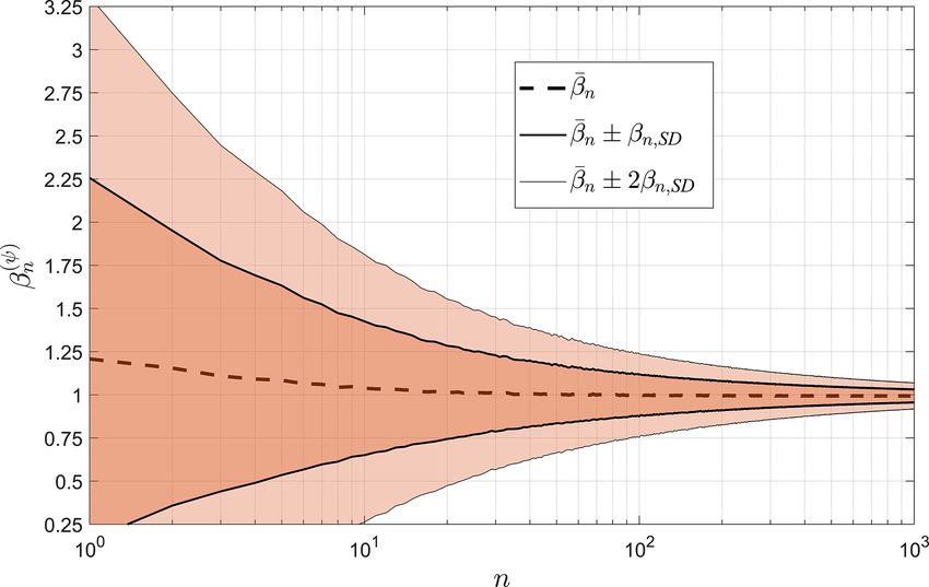
1030                                O. Glowacki and G. B. Deane: Quantifying iceberg calving fluxes with underwater noise

Figure 4. A scheme illustrating the application of passive underwater acoustics to measure iceberg calving fluxes. The study consists of
(1) time-lapse observation of individual calving events; (2) estimation of ice mass loss and block–water impact energy based on the captured
images; (3) recordings of underwater noise at a safe distance from the glacier terminus; and (4) calculation of impact noise energy for given
thermohaline conditions, bathymetry along the transmission path and contribution of noise reflected from the ice cliff.

energy in joules. The selection of the cutoff frequency of the           which are not covered by the bathymetry data (0.1 m reso-
filter (fc = 100 Hz) is discussed in Sect. 4.2. The background           lution) collected during multibeam surveys (Fig. 1). We se-
noise energy, Eac,bckg , for each event was computed analo-              lected five bathymetry profiles, separately for two acoustic
gously using noise segments of the same length as the cor-               buoys, that lie along a straight line between the mooring lo-
responding calving signal, recorded just before the ice block            cation and CTD stations belonging to the transect that is clos-
impact.                                                                  est to the ice cliff. Ocean depths in these sections were then
                                                                         interpolated into a 1 m grid using shape-preserving, piece-
3.3    Hydrographic and bathymetric data                                 wise cubic interpolation (Fritsch and Carlson, 1980; Fig. 3).
                                                                         Despite the fact that a high level of variability in the ther-
An overview of the temperature and salinity structure in                 mohaline structure is expected and there is a lack of detailed
the study site and its influence on the propagation of sound             bathymetry data close to the glacier terminus, the uniquely
throughout the bay has been provided by Glowacki et                      assigned sound speed profile and interpolated bathymetry are
al. (2016). In this study, temperature and salinity profiles             the best available approximation of real conditions prevailing
were taken on 1, 12 and 30 August and 9 September 2016                   during the study period.
with a SAIV SD208 CTD (conductivity, temperature and
depth) probe at 11 points, located on transects perpendicu-              3.4     Attenuation of the calving noise in a glacial bay
lar and parallel to the glacier terminus (red and blue dashed
lines, respectively, in Fig. 1). Sound velocity was calculated           3.4.1    Noise transmission loss
from the CTD data according to the Chen and Millero for-
mulae adopted by UNESCO (Chen and Millero, 1977).                        The underwater sound of a calving event must travel through
   Each calving event has its own, unique set of hydrographic            the water column before reception at an acoustic buoy, typi-
and bathymetric data used for modeling sound propagation,                cally several tens of water depths in range or more. Along its
determined in the following way. Firstly, a median sound                 path, the signal undergoes multiple reflections from the sea
speed profile was calculated from each set of profiles mea-              surface and the sea floor and refracts because of changes in
sured at the same day. Then, a closest median profile was                sound speed caused by the spatial and temporal variability in
assigned to each calving event according to the time of its oc-          the thermohaline structure. These processes result in signifi-
currence. As a result, four consecutive median sound speed               cant loss of the total signal energy and change the frequency
profiles were assigned to 32, 46, 61 and 30 calving events               spectrum of the noise observed at the receiver. These effects
(see Fig. 2). Additional CTD casts were taken in 2017 af-                must be carefully modeled before the calving signature can
ter significant recession of Hansbreen. These profiles pro-              be quantified in terms of ice block impact energy.
vided information on bottom depths in 11 additional posi-                   Here we used the standard ray propagation model Bell-
tions located near the glacier terminus position from 2016,              hop to compute transmission losses, TLprop (Porter, 1987,

The Cryosphere, 14, 1025–1042, 2020                                                            www.the-cryosphere.net/14/1025/2020/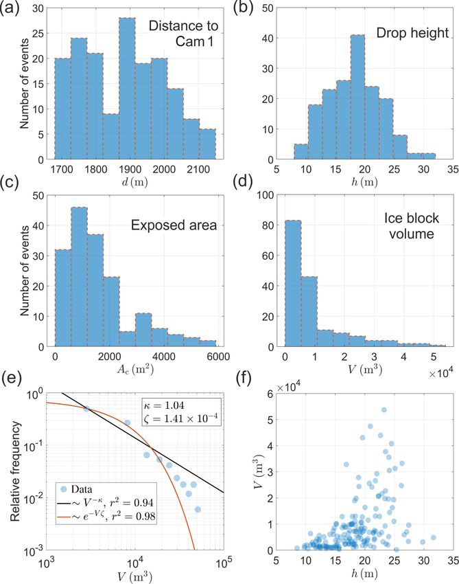
O. Glowacki and G. B. Deane: Quantifying iceberg calving fluxes with underwater noise 1031
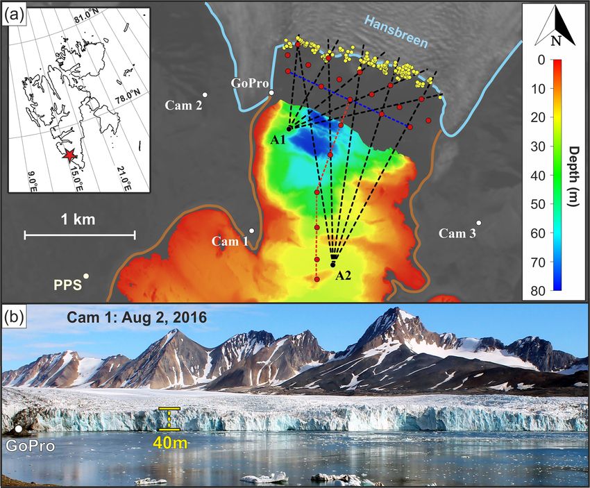
Figure 6. (a–b) Spectrograms of the acoustic signal generated by
the calving event recorded at A1 (a, c, e) and A2 (b, d, f), (c–d) cor-
responding time-averaged spectra of background (red) and calving
(blue) noise, and (e–f) normalized power spectral densities for the
entire calving inventory. The calving event for which spectrograms
and spectra are shown in panels (a)–(d) started on 30 August 2016
at 08:11:08 UTC. A difference of 10, 20 and 40 dB in Pxx corre-
sponds, respectively, to a factor of 10, 100 and 10 000 in acoustic
Figure 5. Histograms of (a) distances between Cam 1 and locations energy. Noise spectra were normalized using maximum values of
of calving events, (b) drop heights, (c) exposed areas of the glacier the calving signal for each event. Solid lines in (e)–(f) show median
terminus and (d) estimated iceberg volumes. (e) Distribution of ice- normalized spectra.
berg volumes divided into 10 bins, presented on log–log scale. The
black line shows best-fit power-law (decay exponent κ) distribu-
tion model. (f) Relationship between iceberg drop height and vol-
ume. The Pearson correlation coefficient is 0.47 and 0.55 for log- probable) transmission loss was computed using the environ-
transformed and non-transformed variables, respectively. mental data described above, assuming a source frequency of
50 Hz, which corresponds to the peak in the source spectrum
(see Fig. 6), and a realistic source depth of 5 mm.
2011). The number of beams was set to 2000, with launch- The longest dimension of the calving icebergs is compa-
ing angles ranging from −80 to 80◦ with respect to the sea rable to or greater than a wavelength over the impact noise
surface. Guided by previous geomorphological studies (Gör- frequencies, and all points distributed along the ice edge and
lich, 1986; Staszek and Moskalik, 2015), we assumed that its close vicinity are considered here to be incoherent noise
the dominant sediment type in the study area is a clayey sources. Accordingly, the incoherent mode of propagation in
silt; density, sound speed and attenuation were taken to be Bellhop was used to compute TLprop . Finally, to investigate
1.4 g cm−3 , 1530 m s−1 and 0.1 dB m−1 kHz−1 , respectively possible variability in TLprop , the simulations were repeated
(Hamilton, 1970, 1976). The absorption of sound in sea- at 100 Hz with the bathymetry-smoothing window changed
water is negligible for the low frequencies considered here to 10λ, ocean depth set to the median water depth and the
(e.g., Ainslie and McColm, 1998). Smoothing bathymetry sound speed profile taken to be each of the four median pro-
and sound velocity profiles is highly recommended when us- files in turn.
ing Bellhop to predict acoustic energy levels (Porter, 1987,
2011). The bathymetry profile for a selected calving event
was spatially smoothed with a moving boxcar filter with 3.4.2 Contribution from terminus-reflected noise
a window size of 20λ, where λ = cf −1 is the wavelength
of sound at the frequency of interest. The median sound The Bellhop model does not easily account for sound re-
speed profile calculated from the set of profiles measured at flected from the underwater part of the glacier terminus,
the closest time to the event occurrence was also spatially which is potentially an important component of the total
smoothed with a moving average over 5 m. A baseline (most acoustic energy received at the buoy. The effect of the glacier
www.the-cryosphere.net/14/1025/2020/ The Cryosphere, 14, 1025–1042, 2020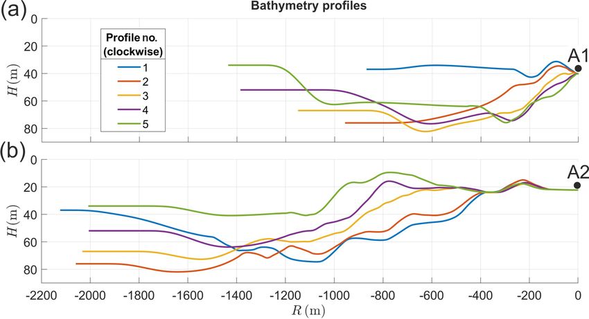
1032                              O. Glowacki and G. B. Deane: Quantifying iceberg calving fluxes with underwater noise

terminus on observed calving noise, TLrefl , is considered          the location of a calving event relative to the glacier–ocean
here.                                                               boundary and position of the acoustic buoy.
   Figure S3 in the Supplement illustrates the direct reflec-          Further analysis was performed using receiver ranges of
tion of sound by the terminus, which is one possible propa-         700 and 1500 m, which correspond to the terminus-receiver
gation path, but there are more, such as a surface or bottom        ranges for the experiment. The source frequency was set to
reflection followed by reflection by the terminus, and so on.       the middle of the analysis band (50 Hz), and the source po-
All possible paths can be enumerated using a series of im-          sition was varied along the terminus at a fixed distance to
age sequences (Deane and Buckingham, 1993) and could, in            the ice cliff of 10 m (Fig. S4b in Supplement). Total energy
principle, be investigated. However, we have simplified the         at the receiver was calculated from the incoherent addition
problem by considering only energy reflected directly by the        of the direct and terminus-reflected paths and compared with
terminus, as shown in Fig. S4 (Supplement). The reasoning           direct path only. The results of this analysis are shown in
behind this simplification is twofold. Firstly, the geometry        Fig. S4c (Supplement). At a range of 1500 m, the maximum
of the problem constrains sound reflected by the bottom fol-        contribution of ice-reflected path is always smaller than 1 dB
lowed by the terminus, and sound reflected by the surface           because of the steep angles of incidence. At a closer distance
between the source and terminus tends to be scattered by            of 700 m, the range of possible angles is extended and a max-
the surface waves and bubbles created by the iceberg im-            imum increase in received calving noise of around 3 dB can
pact. Secondly, the glacier terminus is rough, resulting in         be expected as a “worse-case” scenario. Based on these find-
angle-dependent focusing and scattering. Given these com-           ings, we assumed a typical contribution from ice reflection
plications, which lie beyond the scope of this paper, we have       of TLrefl = 1 dB and corresponding ±1 dB variation around
elected to consider only the effect of energy reflected directly    this level.
from the terminus in comparison with the direct path from
source to receiver. As we will show, the greatest effect from       3.5   Impact energy model
this path over the direct path is a 3 dB increase in sound en-
ergy and a typical effect is less than 1 dB. These levels are       The impact energy model requires an estimate of the total
significantly less than the overall effect of the waveguide or      sound energy radiated by a calving event, which can be cal-
inherent scatter in the intensity of sound generated by indi-       culated from
                                                                                                        −T Ltot
vidual icebergs (see Fig. S5 in Supplement). Moreover, these        Eac,imp = (Eac,obs − Eac,bckg )10     10      ,            (5)
estimates probably represent an upper bound because the ir-
regular shape of the terminus will tend to scatter incident         where TLtot = TLprop + TLrefl is total energy loss in decibels
sound and decrease its contribution when reflected.                 (Clay and Medwin, 1977), which includes both propagation
   The magnitude of sound reflected from the terminus was           loss computed from the Bellhop model and a contribution
calculated using a wavenumber integration technique (see            from energy reflected from the glacier terminus. The sub-
Eq. 4.3.2 in Brekhovskikh and Lysanov, 1982). The ter-              traction of Eac,bckg from the observed impact noise at the
minus surface was assumed to be perfectly flat, and the             hydrophone, Eac,obs , removes background noise energy from
angle-dependent reflection coefficient was estimated us-            the measurement. The factor containing TLtot transforms the
ing standard formulas for a fluid–solid interface (e.g., see        corrected, observed energy into source energy at the impact
Eq. 1.61 in Jensen et al., 2011). The compressional and             location. A total loss of −10 dB, for example, corresponds
shear wave velocities for the ice were taken to be 3840 and         to a decrease of 1 order of magnitude in received energy.
1830 m s−1 , respectively, consistent with those reported by        Based on visual inspection of the scatterplot between Eimp
Vogt et al. (2008) for bubble-free ice (a review of the litera-     and Eac,imp , we used a log−log transformation to improve
ture failed to reveal sound speed values for bubbly ice below       linearity in this relationship. The same type of transforma-
100 Hz). A range of absorption coefficient values were con-         tion was revealed by an application of the Box–Cox algo-
sidered in the analysis: from 0.1 to 1.0 dB λ−1 for longitudi-      rithm, which is often used to normalize regression variables
nal waves and from 0.2 to 2.0 dB λ−1 for shear waves (Ra-           (Box and Cox, 1964). The linear model of conversion be-
jan et al., 1993; Hobæk and Sagen, 2016). Figure S4a in the         tween log-transformed energies is given by
Supplement illustrates the relationship between the angle of
incidence of incoming calving noise and resulting ice reflec-       ln Êac,imp = a + b ln Eimp .                              (6)
tion loss. Three regions can be identified in this figure: (1) up                                                      b , the
                                                                      Having a = ln η and knowing that b ln Eimp = ln Eimp
to 20◦ , the loss is controlled by the ice–water sound speed
                                                                    power-law relationship has a final form given by
ratio and typically reaches a value of approximately 7.5 dB,
(2) between 20 and 55◦ , high attenuation of acoustic energy                     b
                                                                    Êac,imp = ηEimp .                                         (7)
exceeding 15 dB results mainly from absorption in ice, and
finally (3) for larger angles glacier terminus reflects most of        Coefficients a and b could be easily derived from an
the noise energy back to the water. The analysis demonstrates       ordinary least-squares linear regression model using log-
that the ice reflection loss of calving noise depends greatly on    transformed energies as variables. However, both Eimp and

The Cryosphere, 14, 1025–1042, 2020                                                      www.the-cryosphere.net/14/1025/2020/
O. Glowacki and G. B. Deane: Quantifying iceberg calving fluxes with underwater noise 1033
Eac,imp have associated uncertainties, which should be ac- (Fig. 5d). This observation is consistent with previous re-
counted for in the analysis. Therefore, to address this is- ports on the power-law distribution of iceberg sizes in Sval-
sue, we used the unified equations for slope, intercept and bard (Chapuis and Tetzlaff, 2014), Alaska (Neuhaus et al.,
associated standard errors proposed in a model by York et 2019), Greenland (Sulak et al., 2017) and Antarctica (Tour-
al. (2004). This model belongs to the family of errors-in- nadre et al., 2016). A least-mean-squares error analysis of
variables regression models, which include all uncertainties the power-law distribution of iceberg volumes was made us-
and always give an answer that is symmetric for both choices ing log-transformed variables. The best-fit decay exponent of
of dependent and independent variables. Finally, to exclude 1.48 (Fig. 5e) found for the present dataset lies between the
outliers from the analysis, we identified all points for which exponent of 1.69 for Kronebreen, Svalbard, reported by Cha-
uncertainty in acoustic energy calculated with Eq. (5) is not puis and Tetzlaff (2014), and 0.85 for Perito Moreno Glacier,
within 2 standard deviations of the modeled impact noise en- Patagonia, reported by Minowa et al. (2018). However, we
ergy. note that some size ranges can be under- or overrepresented
due to a limited number of unambiguously matched calving
events (169).
4 Results and discussion Ice block volume versus drop height is shown in Fig. 5f.
The highest iceberg volumes are observed for h within the
This section integrates the acoustic and photographic obser- range of 17 and 26 m, which corresponds well to the mid-
vations of calving events into a power-law model that quanti- dle heights of the glacier terminus at the locations of calv-
fies ice mass loss from the noise energy generated by ice- ing events. Inspection of Fig. 5f shows that ice block vol-
berg impact onto the ocean. The model formation begins ume is correlated with drop height; Pearson’s correlation co-
with a discussion of the statistics of iceberg volume and drop efficient is found to be 0.47 and 0.55, respectively, for log-
height estimated from the time-lapse images, leading to es- transformed and non-transformed variables. This is not alto-
timates of the block impact kinetic energy (Sect. 4.1). This gether surprising because the largest blocks of ice cannot fall
is followed by an analysis of the acoustic emission from ice from the bottom of the terminus, whereas the smaller blocks
block impacts in terms of its amplitude–frequency character- of ice are not so constrained. The correlation between drop
istics, resulting in an estimate of the total underwater noise height and iceberg mass is a source of bias in the relationship
energy generated by a calving event (Sect. 4.2). The next between ice block volume and impact energy and must be
section (Sect. 4.3) provides an error analysis of these key accounted for when inverting acoustic recordings of impact
variables in terms of uncertainty in measurements of the en- noise for ice mass loss. This issue is discussed in detail in
vironment, such as bathymetry and thermohaline structure. Sect. 4.5.
The power-law model relating Eimp and Eac,imp is presented
and discussed in Sect. 4.4. Finally, based on this relationship, 4.2 The generation of underwater sound by iceberg
a new methodology is suggested for quantifying the calv- calving
ing flux from the underwater noise of iceberg–water impact
(Sect. 4.5). Figure 6 shows a comparison between power spectral den-
sity estimates for underwater noise from calving and back-
4.1 The statistics of iceberg volume and drop height ground noise recorded by buoys A1 and A2. Spectrograms
of the noise generated by a randomly selected calving event
A total of 169 subaerial calving events were captured by are shown in Fig. 6a and b. The computed difference in time
time-lapse camera and unambiguously identified with acous- of arrival between the two receivers was subtracted from the
tic events (see Sect. 2.2). Individual detachments were un- more distant receiver for better juxtaposition. The two pri-
evenly distributed along the active part of the Hansbreen ter- mary sources of sound in the spectrograms are ice melt noise
minus (Fig. 1). The distance to camera, drop height, exposed and the underwater noise of calving.
terminus area and estimated block volume of the calving in- The signal of ice melt, driven by impulsive bubble release
ventory are summarized in Fig. 5. (Urick, 1971), is most pronounced between 1 and 3 kHz and
The distance between Cam 1 and the locations of block– corresponds well to the spectral bands reported in previous
water impacts varies from 1700 to 2150 m, with an average studies (Deane et al., 2014; Pettit et al., 2015). This signal
of 1880 m (Fig. 5a). The drop height spans 8 to 32 m, with remains stable during the short observation period. The un-
a mean value of h̄ = 18.3 m (Fig. 5b). The range of the ex- derwater noise of calving is a by-product of the interaction of
posed terminus is 125 to 5850 m2 of the ice cliff surface, with the falling iceberg with the ocean. The noise is evident from 2
an average newly exposed area of 1590 m2 (Fig. 5c). Ice- to 8 s in the recording at frequencies below 1 kHz. The acous-
berg volumes were estimated from Ac using Eq. (2) and vary tic intensity varies in both time and frequency. This variabil-
from 0.2 × 10³ to 53.7 × 10³ m3 . The volume distribution is ity is almost certainly driven by different noise production
weighted toward smaller calving events, and approximately mechanisms active at different phases of the calving event
90 % of the ice blocks have a volume of less than 20×103 m3 (see the high variability in power level between 2 and 4 s,
www.the-cryosphere.net/14/1025/2020/ The Cryosphere, 14, 1025–1042, 20201034 O. Glowacki and G. B. Deane: Quantifying iceberg calving fluxes with underwater noise
for example). As pointed out by Bartholomaus et al. (2012), structure is expected to be significant along the longer prop-
low-frequency seismic signals from the impact of ice blocks agation path to A2. Secondly, the signal-to-noise ratio for re-
on the sea surface are generated by three major mechanisms: ceiver A2 is lower and more variable than at A1, as a result
(1) the transfer of momentum from the falling block to sea- of the shallower depth of the hydrophone (22 m at A2 ver-
water, (2) iceberg deceleration due to buoyancy, and (3) the sus 40 m at A1) and greater exposure to noise coming from
collapse of an underwater air cavity and subsequent emer- outside the bay (see Sect. S4c in the Supplement for more
gence of Worthington jets (e.g., Gekle and Gordillo, 2010). details). The increased scatter in calving noise observed at
The last mechanism is only possible during total submer- location A2 resulted in a decrease in correlation between to-
gence of the ice block, the occurrence of which depends tal impact energy and impact noise (see Table S1 in the Sup-
mainly on iceberg dimensions and drop height. Therefore, plement), and data from this buoy are not considered further.
some calving events may not result in the creation of an
air cavity. Moreover, falling icebergs are often fragmented 4.3 Details of error analysis
or impact the water at various angles, which certainly modi-
fies all three mechanisms of noise production. The influence There are two sources of uncertainty for block–water impact
of calving style on sound emission lies beyond the scope of energy and impact noise energy: measurement error and un-
this work but is likely a significant factor in the variability in certainty in the state of the changeable environment, which
sound generation by blocks of similar mass and drop height, is impossible to characterize completely. Estimates of these
as discussed in Sect. 4.4. uncertainties can be made for the various stages of the anal-
The unique patterns in the time and frequency distribu- ysis connecting impact noise to ice mass loss, and these are
tion of calving noise potentially contain information about discussed below.
the details of the calving event. However, attention here is re-
4.3.1 Uncertainty in block–water impact energy
stricted to a single number, which is the time and frequency
integrated energy in the sound field generated by the iceberg Assumptions and approximations need to be made when de-
impact. Calculation of this number requires selection of the termining the kinetic energy of the falling ice block from
start and stop times of the impact noise and the frequency time-lapse images. Uncertainties in estimates of the block–
band over which the noise exceeds background sound levels. water impact energy result mainly from the conversion of
The significant increase in noise power accompanying calv- the exposed area at the glacier terminus into ice block vol-
ing allows easy identification of event start and stop times, ume (see Sect. 3.1). Moreover, additional errors are associ-
and these have been selected manually for each event ana- ated with the details of image analysis, related to the spatial
lyzed (see Sect. S2 in the Supplement). Figure 6c and d show resolution of the time-lapse photography (∼ 80–100 pixels
a 6 s average of noise power spectral density for a calving per terminus height) and imprecise determination of the lo-
signal (blue) and background noise recorded just before the cations of calving events. The total uncertainty in kinetic en-
event (red). There is a difference between the calving and ergy is difficult to estimate accurately due to several factors,
background noise levels at frequencies up to 700 and 400 Hz including but not limited to (1) the irregular shapes of the
for buoys A1 and A2, respectively. The maximum increase icebergs, (2) poorly understood site-to-site variability in the
in received noise power from calving is approximately 40 dB scaling factor C, and (3) space- and time-varying orientation
for both buoys, which corresponds to a factor of 10 000 in of the glacier terminus with respect to the camera. However,
acoustic power. The results in Fig. 6 show that the appropri- following Minowa et al. (2018), we assume that the errors in
ate band of frequencies to consider for calving impact noise Aimg , d, C and h are not larger than 10 %, 5 %, 20 % and 5 %,
ends at around 1 kHz. However, an upper frequency limit respectively. The uncertainty in Ac , computed with Eq. (1),
of 100 Hz was applied in further analysis to yield the high- is 14 %. Then, since uncertainties in the estimates of ice vol-
est correlation between the impact energy and the received umes and drop heights are dependent, the total error bound
acoustic energy. in the kinetic energy of the impacting ice block is estimated
The variability in calving noise power across the entire to be approximately 33 %.
dataset is shown in Fig. 6e and f. The normalized power
spectral densities of calving events and background noise 4.3.2 Errors in calving-generated acoustic energy
are plotted as blue and red dots, respectively. A normaliza-
tion factor is chosen for each calving event and taken to be Uncertainties in estimates of the iceberg impact noise re-
the highest power level in decibels during the event. The sult from three major sources: (1) spatial and temporal vari-
same normalization factor is used for both calving and back- ability in the thermohaline structure in the glacial bay (see
ground noise. Calving signatures are clearly distinguishable Fig. 2a–d), (2) complicated bathymetry along the propaga-
from the background noise across the entire dataset. How- tion path, which depends on the location of calving event (see
ever, the calving noise power is noticeably more variable at Fig. 3), and (3) angular and frequency dependence of sound
receiver A2 than A1. There are two possible reasons for this reflection from the underwater part of the glacier terminus
discrepancy. Firstly, spatial dependency of the thermohaline (see Fig. S4 in Supplement). Considering both transmission
The Cryosphere, 14, 1025–1042, 2020 www.the-cryosphere.net/14/1025/2020/O. Glowacki and G. B. Deane: Quantifying iceberg calving fluxes with underwater noise 1035
and reflection losses, the total loss of acoustic energy gener-
ated by block–water interaction, TLtot , ranges from −47 to
−57 dB (see Fig. S5 in the Supplement), corresponding to
a factor of 10−5 and 10−6 in acoustic energy at the source
across the entire inventory of calving events. We combined
variability in transmission and ice reflection losses for the
entire calving inventory to estimate a representative uncer-
tainty of 33 % in acoustic energy for each individual calving
event at its source.
4.4 Relationship between the block–water impact and
acoustic energy
Estimating calving ice mass flux from calving noise is based
on the idea that these two quantities are correlated. Figure 7
shows a scatterplot of impact noise, Eac,imp , against impact
kinetic energy, Eimp , for the entire dataset. The dashed black
line shows the result of a regression analysis of the power-law
relationship shown in the figure legend. The acoustic energy
generated by a calving event was calculated from the acoustic
pressure time series using Eqs. (4) and (5) with manual selec-
tion of integration time (see Sect. S2 in the Supplement) and
after low-pass filtering at a cutoff frequency of 100 Hz (see
Sect. 4.2). The kinetic energies of the falling ice blocks were
derived from Eq. (3) using their masses and drop heights es-
timated from the camera data (see Sect. 4.1).
Figure 7. Relationship between the block–water impact energy
The range of energy estimates is large, roughly 2.5 orders
and underwater acoustic emission below 100 Hz. Uncertainties are
of magnitude for both, and there is clearly a strong corre- marked with blue whiskers and were estimated to be 33 % for both
lation between the energies across their entire range. The variables. The remaining scatter in impact energy is most likely
regression coefficient r = 0.76 was found between the log- caused by different calving styles and an associated variability in
transformed variables for p < 0.0001. If uncorrected calving source mechanisms. The results with inclusion of outliers are shown
noise energy and signal duration are used instead of Eac,imp , in Fig. S6 in the Supplement (see text for details).
the correlation drops to 0.71 and 0.61, respectively (Table S1
in the Supplement). After removing two outliers and apply-
ing an error-in-variables linear regression (see Sect. 3.5 for to the acoustic receiver. A low conversion efficiency is con-
details), the best functional relationship between acoustic en- sistent with observations reported for other physical mech-
ergy and impact energy was found to be a power-law rela- anisms of underwater noise generation. For example, only
tionship given by Eq. (7), where η = 8 × 10⁻⁷ ± 60 % and ∼ 10−8 of the energy dissipated by a breaking surface wave
b = 0.92±3 %, respectively, for the multiplication factor and on the ocean is radiated as sound (Loewen and Melville,
exponent of the power law. For completeness, this analy- 1991). Similarly, the conversion efficiency of the impact en-
sis was repeated, including the two identified outliers, and ergy of a 1–5 mm scale raindrop falling on the sea surface to
the results are shown in Fig. S6 (Supplement). Glowacki et underwater impact noise is in the range 10−9 to 10−8 (see
al. (2015) previously reported η = 5.16 × 10⁻¹⁰ and b = 1, Eq. 4.6 in Guo and Ffowcs Williams, 1991, and Gunn and
which gives an impact energy that is 2.5 orders of magni- Kinzer, 1949).
tude higher in comparison to the results presented here (see Despite a strong correlation between impact energy and
Fig. S7 in Supplement). This discrepancy is due to the overly impact noise, there is also a significant scatter in impact noise
simplified propagation geometry assumed in the earlier study energy (roughly a factor of 10) for a given value of kinetic en-
– simple cylindrical spreading loss and no sound reflection ergy. This spread in values can be only partly explained by
from ice terminus – which resulted in an underestimate of errors in the energy estimates, which are indicated by blue
the impact noise energy. whiskers in the Fig. 7. The scatter is presumably caused by
The multiplication factor η can be thought of as a conver- differences in noise generation between individual calving
sion efficiency of kinetic energy of a falling iceberg to impact events. The consequence is that estimating the impact en-
noise energy. The small value of η shows that only a tiny ergy of an individual calving event from the total noise en-
fraction of the ice block energy is transformed into underwa- ergy it radiates is accompanied with significant uncertainty.
ter sound, which then propagates from the point of impact However, because of the overall strong correlation between
www.the-cryosphere.net/14/1025/2020/ The Cryosphere, 14, 1025–1042, 20201036 O. Glowacki and G. B. Deane: Quantifying iceberg calving fluxes with underwater noise
noise and impact kinetic energy, it is possible to predict the We are left with the problem of computing ĥ. To address
total impact energy summed over a finite number of calv- this issue, a new variable α̂ is defined by
ing events, provided the inventory is large enough. The un- N
N N
!
certainty in individual events tends to average out if enough
X 1 X X
α̂ = ĥ h̄−1 = hj M̂j hj M̂j , (11)
events are considered, as discussed in Sect. 4.5. j =1
N j =1 j =1
4.5 Estimation of ice mass loss from the calving noise where h̄ is an observed, average drop height. Let us now as-
sume that, for sufficiently large N, α̂ can be approximated
Figure 7 and Eq. (7) show that the relationship between ice- by
berg impact energy and calving noise can be modeled ro- N
N N
!
bustly with a power-law relationship, providing a means of
X 1 X X
α̂ ≈ hj Mj hj Mj . (12)
estimating impact energy from calving noise. Although there j =1
N j =1 j =1
is significant variability in doing this on an event-by-event
basis, low-error estimates of cumulative impact energy can The right-hand side of Eq. (12) is in terms of iceberg mass
be made using Eq. (7) if enough events are added together. inferred from the camera observations, providing a means
Once found, the cumulative impact energy can be converted of computing the mass-weighted drop height, ĥ = α̂ h̄, on a
into an estimate of iceberg calving flux as follows. glacier-by-glacier basis. The constant α̂ and resulting mass-
The cumulative modeled ice mass loss from N observed weighted average drop height are estimated to be 1.13 and
calving events is related to the cumulative impact energy, as 20.7 m for Hansbreen.
inferred from the acoustic signal, by Equation (10) for the cumulative calving mass flux con-
tains significant uncertainty when N is small because of
N
X N
X the large scatter in the total underwater sound energy gen-
g hj M̂j = Êimp, j , (8) erated by calving events with similar impact energies (see
j =1 j =1 Fig. 7), but the uncertainty reduces as N increases. How
large must N be to achieve a desired degree of uncertainty?
where g is the acceleration due to gravity, hj is the height To answer this question, a Monte Carlo simulation of cumu-
of the center of mass of the j th iceberg before separation lative ice mass loss was performed using n calving events
from the glacier terminus, M̂j is the mass of j th iceberg de- randomly selected (with replacement) from the entire inven-
termined from its underwater impact noise and Êimp,j is the tory of calving observations (for which N = 169). This se-
kinetic energy of impact of the j th iceberg. The cumulative lection is repeated ψmax times (ψ = {1, . . ., ψmax }) for each
ice mass lost through calving would be trivial to compute n = {1, . . ., nmax }, noting that the total number of possible
from Eq. (8) if the mean iceberg drop height were indepen- sets of calving events (and associated cumulative kinetic en-
dent of the iceberg mass, but this is not the case (see Fig. 5f). ergies and masses) is given by
Icebergs that extend a significant fraction of the exposed ter-
n+N −1
(n + N − 1) !
minus height have a minimum drop height that is larger than C= = . (13)
n n! (N − 1) !
the minimum drop height possible for smaller icebergs. For
this (and possibly other) reasons there is a correlation be- From Eq. (10), the cumulative mass sum for a given num-
tween iceberg drop height and iceberg mass, the consequence ber of randomly selected calving events n and iteration ψ is
of which is that hj cannot be moved outside the sum on the n n
X (ψ) 1 X (ψ)
left-hand side of Eq. (8). The correlation is dealt with by in- M̂i = Êimp, i , (14)
troducing the mass-weighted drop height: i=1 g ĥ i=1
N N
X where ĥ is calculated from Eqs. (11) and (12) using the N =
X (ψ)
ĥ = hj M̂j M̂j . (9) 169 observed calving events. The modeled mass M̂i in
j =1 j =1 Eq. (14) corresponds to M̂j in Eq. (10), where 1 ≤ j ≤ 169.
The inferred, cumulative ice mass normalized by the cumu-
It follows immediately from Eqs. (8) and (9) that the cu- lative ice mass measured with the camera is then given by
mulative mass sum is given by n
X n
(ψ) (ψ)
X
βn(ψ) = M̂i Mi , (15)
N N
X 1 X i=1 i=1
M̂j = Êimp, j , (10)
j =1 g ĥ j =1 where β, for a specified n and averaged over ψmax iterations,
can be expressed as
which provides a means of computing the calving flux, since ψmax X n
X n
!
the kinetic energy of iceberg impact can be estimated from 1 X (ψ) (ψ)
β̄n = M̂ Mi . (16)
its underwater noise using Eq. (7). ψmax ψ=1 i=1 i i=1
The Cryosphere, 14, 1025–1042, 2020 www.the-cryosphere.net/14/1025/2020/You can also read