Oceanic response to the consecutive Hurricanes Dorian and Humberto (2019) in the Sargasso Sea
←
→
Page content transcription
If your browser does not render page correctly, please read the page content below
Nat. Hazards Earth Syst. Sci., 21, 837–859, 2021
https://doi.org/10.5194/nhess-21-837-2021
© Author(s) 2021. This work is distributed under
the Creative Commons Attribution 4.0 License.

Oceanic response to the consecutive Hurricanes Dorian and
Humberto (2019) in the Sargasso Sea
Dailé Avila-Alonso1,2 , Jan M. Baetens2 , Rolando Cardenas1 , and Bernard De Baets2
1 Laboratoryof Planetary Science, Department of Physics, Universidad Central “Marta Abreu” de Las Villas,
54830, Santa Clara, Villa Clara, Cuba
2 KERMIT, Department of Data Analysis and Mathematical Modelling, Faculty of Bioscience Engineering,

Ghent University, 9000 Ghent, Belgium

Correspondence: Dailé Avila-Alonso (davila@uclv.cu)

Received: 7 September 2020 – Discussion started: 27 October 2020
Revised: 18 December 2020 – Accepted: 13 January 2021 – Published: 2 March 2021

Abstract. Understanding the oceanic response to tropical cy-     1   Introduction
clones (TCs) is of importance for studies on climate change.
Although the oceanic effects induced by individual TCs have
been extensively investigated, studies on the oceanic re-        Hurricanes and typhoons (or more generally, tropical cy-
sponse to the passage of consecutive TCs are rare. In this       clones (TCs)) are among the most destructive natural phe-
work, we assess the upper-oceanic response to the passage of     nomena on Earth, leading to great social and economic losses
Hurricanes Dorian and Humberto over the western Sargasso         (Welker and Faust, 2013; Lenzen et al., 2019), as well as eco-
Sea in 2019 using satellite remote sensing and modelled data.    logical perturbations of both marine and terrestrial ecosys-
We found that the combined effects of these slow-moving          tems (Fiedler et al., 2013; de Beurs et al., 2019; Lin et al.,
TCs led to an increased oceanic response during the third        2020). Given the devastating effects of TCs, the question of
and fourth post-storm weeks of Dorian (accounting for both       how they will be affected by climate change has received
Dorian and Humberto effects) because of the induced mix-         considerable scientific attention (Henderson-Sellers et al.,
ing and upwelling at this time. Overall, anomalies of sea sur-   1998; Knutson et al., 2010; Walsh et al., 2016). Modelling
face temperature, ocean heat content, and mean temperature       studies project either a decrease in TC frequency accompa-
from the sea surface to a depth of 100 m were 50 %, 63 %,        nied by an increased frequency of the strongest storms or
and 57 % smaller (more negative) in the third–fourth post-       an increase in the number of TCs in general, depending on
storm weeks than in the first–second post-storm weeks of         the spatial resolution of the models (Knutson et al., 2010;
Dorian (accounting only for Dorian effects), respectively. For   Camargo and Wing, 2016; Walsh et al., 2016; Zhang et al.,
the biological response, we found that surface chlorophyll a     2017; Bacmeister et al., 2018; Bhatia et al., 2018). In any
(chl a) concentration anomalies, the mean chl a concentra-       case, an assessment of the impact of climate change on fu-
tion in the euphotic zone, and the chl a concentration in the    ture TC activity needs to be based on whether or not the past
deep chlorophyll maximum were 16 %, 4 %, and 16 % higher         and present changes in climate have had a detectable effect
in the third–fourth post-storm weeks than in the first–second    on TCs to date (Walsh et al., 2016).
post-storm weeks, respectively. The sea surface cooling and         The ocean is the main source of energy for TC intensifica-
increased biological response induced by these TCs were sig-     tion; hence, changes in oceanic environments considerably
nificantly higher (Mann–Whitney test, p < 0.05) compared         affect TC activity (Knutson et al., 2010; Huang et al., 2015;
to climatological records. Our climatological analysis reveals   Sun et al., 2017; Trepanier, 2020). Sea surface temperature
that the strongest TC-induced oceanographic variability in       (SST) and ocean heat content (OHC) have risen significantly
the western Sargasso Sea can be associated with the occur-       over the past several decades in regions of TC formation
rence of consecutive TCs and long-lasting TC forcing.            (Santer et al., 2006; Defforge and Merlis, 2017; Trenberth
                                                                 et al., 2018; Cheng et al., 2019; Zanna et al., 2019; Chih and

Published by Copernicus Publications on behalf of the European Geosciences Union.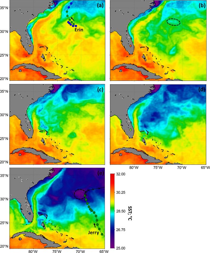
838                              D. Avila-Alonso et al.: Oceanic response to the Hurricanes Dorian and Humberto (2019)

Wu, 2020). Accordingly, TC lifetime maximum intensity sig-        storms on upper-ocean oceanographic conditions. Although
nificantly increased during 1981–2016 for both the Northern       there have been extensive studies investigating the oceanic
Hemisphere and Southern Hemisphere (Song et al., 2018).           response described above to the passage of individual TCs,
More specifically, both the frequency and intensity of TCs in     the effects induced by consecutive TCs have been much less
the North Atlantic basin increased over the past few decades      documented (Wu and Li, 2018; Ning et al., 2019). More
(Deo et al., 2011; Walsh et al., 2016), while a significant in-   specifically, extensive and long-lasting SST cooling and in-
crease in TC intensification rates in the period 1982–2009        tense post-storm phytoplankton blooms after the passage of
has been documented with a positive contribution from an-         consecutive TCs have been documented in the northwestern
thropogenic forcing (Bhatia et al., 2019).                        Pacific Ocean (e.g. Wu and Li, 2018; Ning et al., 2019; Wang
   The most recent Atlantic hurricane seasons have shown          et al., 2020). However, to the best of our knowledge, there are
well above normal activity (Trenberth et al., 2018; Bang          no previous studies assessing the biological response to con-
et al., 2019). For instance, the 2017 hurricane season was        secutive TCs in the western Sargasso Sea.
extremely active with 17 named storms (1981–2010 median              Given that the greatest ocean warming is projected to oc-
is 12.0), 10 hurricanes (median is 6.5), and six major hurri-     cur by the end of the century (Cheng et al., 2019), we may
canes (Klotzbach et al., 2018, median is 2.0). It will be re-     anticipate a further increase in TC intensity and/or frequency.
membered for the unprecedented devastation caused by the          The assessment of the oceanic response to TCs has been a hot
major Hurricanes Harvey, Irma, and Maria, breaking many           topic given its importance for studies on climate change, eco-
historical records (Todd et al., 2018; Trenberth et al., 2018;    logical variability, and environmental protection (Fu et al.,
Bang et al., 2019). This high activity was associated with un-    2014). More specifically, insights into the phytoplankton re-
usually high SST in the eastern Atlantic region, where many       sponse to severe weather events are essential in order to as-
storms developed, together with record-breaking OHC val-          certain the capacity of the oceans to absorb carbon diox-
ues favouring TC intensification (Lim et al., 2018). In ad-       ide through photosynthesis (Davis and Yan, 2004). Hence,
dition, the 2019 hurricane season was relevant because of         several studies have assessed the oceanic response to re-
the high number of named storms (18 storms) and the devel-        cent major hurricanes in the North Atlantic basin (e.g. Tren-
opment of long-lasting Hurricane Dorian, which broke the          berth et al., 2018; Miller et al., 2019b; Avila-Alonso et al.,
record for the strongest Atlantic hurricane outside the trop-     2020; Hernández et al., 2020) and others in very active hur-
ics (Klotzbach et al., 2019; Ezer, 2020, > 23.5◦ N). About        ricane seasons such as in 2005 (e.g. Oey et al., 2006, 2007;
2 weeks after the passage of Dorian across the western Sar-       Shi and Wang, 2007; Gierach and Subrahmanyam, 2008). In
gasso Sea, TC Humberto moved across this area. The interac-       this work, we assess the upper-oceanic responses induced by
tion of two storms closely related in time and space provides     Hurricanes Dorian and Humberto in the western Sargasso
an in situ experiment for studying oceanic response (Bara-        Sea in 2019. This gives insights into the implications of a
nowski et al., 2014).                                             simultaneous increase in both the frequency and intensity of
   Over oceans, TC-induced wind forcing mixes the surface         TCs in the North Atlantic basin.
layer, deepens the mixed layer, and uplifts the thermocline,
leading to a decreased upper-ocean temperature and heat
potential (Price, 1981; Shay and Elsberry, 1987; Trenberth        2     Materials and methods
et al., 2018). Vertical mixing and upwelling also lead to an
                                                                  2.1    Study area
increased abundance of surface phytoplankton due to entrain-
ment of nutrient-rich waters from the nitracline to the ocean     The Sargasso Sea is the part of the North Atlantic Ocean
surface and/or entrainment of phytoplankton from the deep         (known as the North Atlantic gyre) that is bounded by the
chlorophyll maximum (DCM) (Babin et al., 2004; Walker             surrounding clockwise-rotating system of major currents, i.e.
et al., 2005; Gierach and Subrahmanyam, 2008; Shropshire          the North Atlantic Current in the north, the Gulf Stream in the
et al., 2016). The nutrient influx stimulates phytoplankton       west, the North Atlantic Equatorial Current in the south, and
growth and can lead to phytoplankton blooms lasting sev-          the Canary Current in the east (Deacon, 1942; Laffoley et al.,
eral days after the TC passage in the oligotrophic oceanic        2011). Hence, the Sargasso Sea essentially lies between the
waters (Babin et al., 2004; Hanshaw et al., 2008; Shropshire      parallels 20–35◦ N and the meridians 30–70◦ W (Augustyn
et al., 2016). Moreover, rainfall associated with these ex-       et al., 2013). We considered the western Sargasso Sea as our
treme meteorological phenomena modulates surface cooling          study area (shown in Fig. 1), since it was affected by Dorian
and phytoplankton blooms since rainfall freshens the near-        and Humberto.
surface water, thus increasing stratification and influencing
vertical mixing (Lin and Oey, 2016; Liu et al., 2020). From       2.2    Synoptic history of Dorian and Humberto
satellite imagery, an increase in phytoplankton abundance is
identified as an elevated chlorophyll a (chl a) concentration.    Dorian originated from a tropical wave that moved off
Distinguishing between mechanisms inducing changes in chl         the west coast of Africa on 19 August 2019. The wave
a concentration is crucial to understanding the impact of         crossed the tropical Atlantic, becoming a tropical depres-

Nat. Hazards Earth Syst. Sci., 21, 837–859, 2021                                  https://doi.org/10.5194/nhess-21-837-2021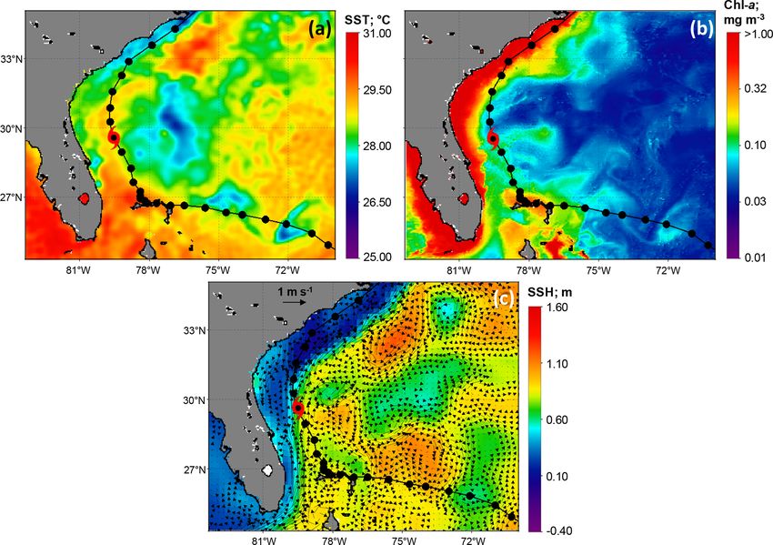
D. Avila-Alonso et al.: Oceanic response to the Hurricanes Dorian and Humberto (2019)                                            839

sion on 24 August 24 at 06:00 UTC at about 1296 km east-            in order to account for the oceanic response in the Sargasso
southeast of Barbados and a tropical storm at 18:00 UTC             Sea, we restricted the study area to the deep waters to the
that day. Dorian’s intensity increased further while moving         right of Dorian’s trajectory. Given that upwelling, cooling,
west-northwest, reaching hurricane category by 27 Septem-           and deepening of the isothermal layer are more intense on
ber and major hurricane category by 30 September, while             the right side of a TC’s trajectory in the Northern Hemi-
being centred about 713 km east of the northwestern Ba-             sphere (Price, 1981; Hanshaw et al., 2008; Gierach and Sub-
hamas (Fig. 1a). Dorian became a category 5 hurricane on            rahmanyam, 2008; Fu et al., 2014), our asymmetric approach
the Saffir–Simpson hurricane scale in the northwestern Ba-          captures the strongest oceanic response. In addition to these
hamas on 1 September with estimated winds of 296 km h−1 .           Lagrangian measurements along Dorian’s trajectory, we also
At this time, it moved very slowly westward, making landfall        investigated the oceanic response in a square area (Eulerian)
on Grand Bahama on 2 September with winds of 287 km h−1             located to the right of its trajectory (Fig. 1b), where a con-
(Fig. 1a). Dorian remained stationary over this area, weak-         siderable post-storm sea surface cooling was observed. The
ening to categories 4 and 3 (Fig. 1a) because of its interac-       strongest oceanic response accounting for the combined ef-
tion with land and the induced ocean cooling. Then, it turned       fect of Dorian and Humberto was observed in this square
northwestward and started moving along the east of Florida          area since it was affected by the intensive winds near the
during the period from 3–5 September as a category 2, but           centre of Dorian, and it was crossed by Humberto. In con-
as its core moved over the Gulf Stream, Dorian regained             trast, the entire area along Dorian’s trajectory was affected
strength and reached category 3 again offshore of the coasts        by Humberto to a lesser extent, especially the waters sur-
of Georgia and South Carolina (Fig. 1a). Afterwards, Do-            rounding Grand Bahama since Humberto crossed semi-disc 1
rian made landfall over Cape Hatteras on 6 September with           (see Fig. 1). Moreover, storm surge and saltwater inunda-
157 km h−1 and left the Sargasso Sea that day, when moving          tion were reported along the east coast of Florida following
beyond 35◦ N (Avila et al., 2020).                                  the passage of Humberto (Stewart, 2020), indicating that this
   On the other hand, Humberto primarily originated from a          area was also exposed to its forces.
weak tropical wave that started off the west coast of Africa           We assessed the daily response of the oceanographic vari-
on 27 August and moved westward across the tropical At-             ables before, during, and after the passage of Dorian. We
lantic, approaching the Lesser Antilles on 4 September. By          considered the pre-storm week (i.e. days −10 to −3 before
31 September it became a tropical depression east of the            hurricane passage) as a benchmark for comparison with the
central Bahamian island of Eleuthera at 18:00 UTC, and 6 h          four post-storm weeks (i.e. from days 0 to 30, where day
later it became a tropical storm (Fig. 1a). Then, Humberto          0 refers to the day the hurricane entered the study area) in
turned northwestward and maintained that direction for the          agreement with previous studies (Menkes et al., 2016; Avila-
next 48 h at a slow translation speed. It reached hurricane         Alonso et al., 2019). For the square area, we considered day 0
category on 16 September about 278 km east-northeast of             as the day that Dorian started to impact it, i.e. as soon as there
Cape Canaveral, Florida (Fig. 1a). At this point, Humberto          was overlap of the 200 km radius semi-discs and the square
started to move east-northeastward, strengthening to a major        polygons. Overall, the first two post-storm weeks account for
hurricane on 18 September (Fig. 1a). Thereafter, Humberto           Dorian-induced oceanic effects, while the third and fourth
weakened steadily and became an extratropical cyclone by            post-storm weeks account for the combined effects of both
20 September (Stewart, 2020).                                       Dorian and Humberto. Daily arithmetic means of the stud-
                                                                    ied variables were computed along Dorian’s trajectory and in
2.3   Methodology                                                   the square study area. For the former, the mean values of the
                                                                    consecutive semi-discs were averaged to retrieve the daily
We analysed the oceanic response along the trajectory of            mean along the entire hurricane trajectory, in agreement with
Dorian in 200 km radius semi-discs centred at consecutive           Babin et al. (2004).
hurricane positions in the 20–35◦ N latitudinal band (limits
of the Sargasso Sea; Fig. 1b). We followed this asymmet-            2.4     Data
ric approach due to the fact that Dorian moved close to the
east coast and shelf waters of the United States of Amer-           2.4.1    Response variables
ica (USA); thus, the waters to the left side of its trajectory
can be considered optically complex waters (i.e. Case 2 wa-         We considered SST and chl a concentration as the main
ters of the classification of Morel, 1980), which limit the         physical and biological response variables, respectively, as in
use of ocean colour data. On the other hand, coastal–shelf          previous studies in the region (e.g. Babin et al., 2004; Shrop-
and oceanic waters respond differently to the passage of TCs        shire et al., 2016). SST data were derived from the Opera-
(Zhao et al., 2015). For instance, coastal areas are strongly       tional SST and Sea Ice Analysis (OSTIA) Near Real Time
affected by freshwater discharge and flooding, leading to a         level-4 product (Donlon et al., 2012), provided by the Coper-
high concentration of nutrients and post-storm phytoplank-          nicus Marine Environment Monitoring Service (CMEMS,
ton productivity (Farfán et al., 2014; Paerl et al., 2019). Thus,   http://marine.copernicus.eu, last access: May 2020). OSTIA

https://doi.org/10.5194/nhess-21-837-2021                                     Nat. Hazards Earth Syst. Sci., 21, 837–859, 2021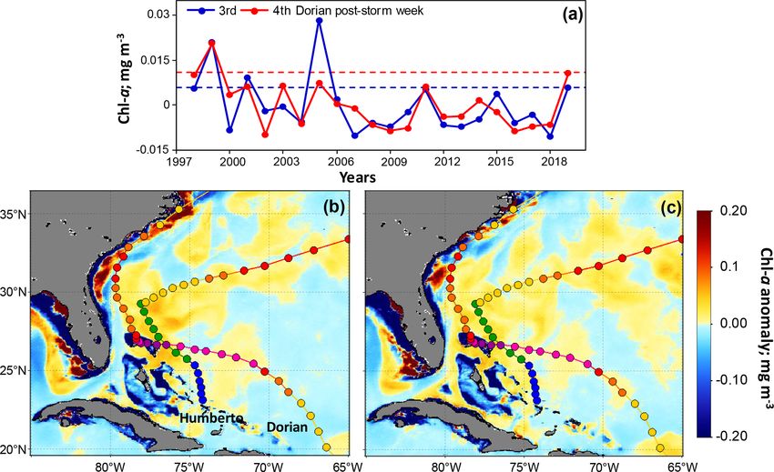
840                                D. Avila-Alonso et al.: Oceanic response to the Hurricanes Dorian and Humberto (2019)

Figure 1. (a) Trajectory of tropical cyclones (TCs) Dorian and Humberto (2019). Colours indicate the TC category (i.e. L: low-pressure
system; TD: tropical depression; TS: tropical storm; H1–H5: Saffir–Simpson hurricane categories). Numbers along trajectories indicate the
day/month. (b) The 200 km semi-discs along Dorian’s trajectory and the square area in the western Sargasso Sea. Red semi-discs 1 and 2
indicate the areas where chlorophyll a concentration profiles were analysed.

merges both infrared and microwave radiometer data, to-                   We used daily OHC data from the Systematically Merged
gether with in situ observations, at a spatial resolution of           Regional Atlantic Temperature and Salinity (SMARTS) cli-
0.05◦ × 0.05◦ .                                                        matology adjusted to a two-layer reduced gravity model at a
   We used the CMEMS GlobColour multi-satellite merged                 spatial resolution of 0.25◦ ×0.25◦ (Meyers et al., 2014) (data
data of near-real-time chl a concentration (level-4 cloud free         available at ftp://ftp.nodc.noaa.gov/pub/data.nodc/sohcs, last
product), which is based on a spatial and temporal inter-              access: May 2020). SMARTS blends temperature and salin-
polation of the level-3 product at a spatial resolution of             ity fields from the World Ocean Atlas 2001 (WOA01) and
0.0417◦ × 0.0417◦ (Garnesson et al., 2019b, a). The chl a              the Generalized Digital Environmental Model (GDEM) ver-
analyses involve multiple chl a algorithms, i.e. CI algorithm          sion 3.0 based on their performance compared to in situ mea-
for oligotrophic waters (Hu et al., 2012) and OC5 algorithm            surements (Meyers et al., 2014). SMARTS estimations of
for mesotrophic and coastal waters (Gohin et al., 2002; Go-            OHC during hurricane seasons show little bias and low nor-
hin, 2011). The CI and OC5 continuity is ensured using the             malized root-mean-squared difference (RMSD normalized
same approach as that utilized by NASA. When the chl a                 by the mean of the local in situ observations) in the North At-
concentration is in the range from 0.15 to 0.2 mg m−3 , a lin-         lantic basin in general, with the lowest values in the western
ear interpolation is used (Garnesson et al., 2019b). The al-           Sargasso Sea (e.g. RMSD ≈ 0.3; see Fig. 2-16 in Shay et al.,
gorithm validation has shown a good relationship between in            2019). Temperature profiles were derived from the Global
situ measurements and satellite observations of chl a con-             Ocean Physics Analysis and Forecasting product at a spatial
centration, while daily level-4 products in general show a             resolution of 0.083◦ × 0.083◦ , provided by Mercator Ocean
low bias (0.04) and a coefficient of determination of 0.71 at          and distributed by CMEMS. This product uses version 3.1 of
global scale (Garnesson et al., 2019a).                                the NEMO (Nucleus for European Modelling of the Ocean)
   Moreover, we also investigated the subsurface oceano-               ocean model and has 50 vertical levels (22 levels within the
graphic variability by analysing data of the OHC, which cor-           upper 100 m) with a decreasing resolution from 1 m at the sea
respond to the integrated thermal energy from the sea surface          surface to 450 m into the deep ocean (Lellouche et al., 2016).
to 26 ◦ C isotherm depth (Leipper and Volgenau, 1972; Price,              The chl a profiles were obtained from the CMEMS Global
2009), and the average temperature from the sea surface to a           Biogeochemical Analysis and Forecast product of Merca-
depth of 100 m (T100 , a typical depth of vertical mixing by a         tor Ocean. This product is a global biogeochemical simula-
category 3 hurricane) (Price, 2009). The latter has been sug-          tion result (at 0.25◦ × 0.25◦ spatial resolution) obtained us-
gested as an adequate variable to identify subsurface thermal          ing the PISCES (Pelagic Interactions Scheme for Carbon and
fields (Price, 2009), so we can draw sound conclusions on              Ecosystem Studies) model which is part of the NEMO model
the subsurface cooling as a consequence of the TCs. Simi-              (Lamouroux et al., 2019). The vertical grid of this product
larly, we analysed chl a concentration profiles to assess the          has 50 levels (ranging from 0 to 5500 m), with a resolution
post-storm biological response throughout the euphotic zone            of 1 m near the sea surface and 400 m into the deep ocean
(0–200 m).                                                             (Lamouroux et al., 2019). Such chl a concentration profiles
                                                                       have shown good agreement with both satellite and in situ

Nat. Hazards Earth Syst. Sci., 21, 837–859, 2021                                        https://doi.org/10.5194/nhess-21-837-2021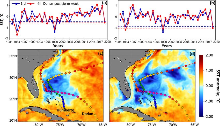
D. Avila-Alonso et al.: Oceanic response to the Hurricanes Dorian and Humberto (2019)                                          841

measurements. Moreover, the depth of the DCM is quite ac-         speed and rainfall on the upper-ocean response, we consider
curately simulated for the North Atlantic subtropical gyre        that through the assessment of the MLD and D20 variability
(Lamouroux et al., 2019).                                         the effects of the above-mentioned atmospheric variables are
                                                                  taken into account. It has been suggested that wind-driven
2.4.2   Drivers of ocean cooling                                  processes (i.e. vertical mixing and upwelling) govern the
                                                                  post-storm SST cooling in the waters surrounding Cuba due
Post-storm SST cooling is a very complex process, involving       to the high and statistically significant correlation of wind
hydrodynamic (vertical mixing and upwelling) and thermo-          speed and SST, as well as the consistent temporal variabil-
dynamic (surface heat flux) processes (Vincent et al., 2012a).    ity of wind speed, MLD, D20, and SST anomalies during
Taking into account that cooling as a consequence of sur-         and after the passage of a hurricane (Avila-Alonso et al.,
face heat loss is more relevant towards the shallow waters        2019, 2020). Moreover, model simulations have revealed that
of the continental shelf (Morey et al., 2006; Ezer, 2018; Wei     TC rainfall can reduce the post-storm MLD, thus reducing
et al., 2018), we assessed the variability of the mixed layer     cold water entrainment (Jacob and Koblinsky, 2007; Jourdain
and the thermocline displacement induced by Dorian and            et al., 2013). Overall, fresh rainwater affects vertical stability
Humberto in order to identify the drivers of the post-storm-      and therefore modulates ocean mixing (Jacob and Koblinsky,
induced cooling. The mixed-layer depth (MLD) data were            2007; Jourdain et al., 2013).
derived from the Global Ocean Physics Analysis and Fore-             Given the heterogeneous nature of the datasets used in
casting product distributed by CMEMS. MLD is defined by           this study, i.e. satellite and modelled data obtained using
sigma theta considering a variable threshold criterion (equiv-    different methods at different spatial resolutions, we focus
alent to a 0.2 ◦ C decrease), i.e. the depth where the density    on highlighting general spatio-temporal patterns of the anal-
increase compared to density at 10 m depth corresponds to         ysed variables, since some specific dynamics may be a con-
a temperature decrease of 0.2 ◦ C in local surface conditions     sequence of this heterogeneity.
(Chune et al., 2019).
   Upwelling and downwelling regimes can be identified by
analysing the fluctuations in 20 ◦ C isotherm depth (D20;
Jaimes and Shay, 2009, 2015), since D20 generally occurs          3     Results
within the area of maximum vertical temperature gradient in
the tropical ocean. Therefore, D20 is considered a proxy for      3.1     Physical response
the thermocline (Delcroix, 1984; Reverdin et al., 1986; Sea-
ger et al., 2019). The subtropical western Sargasso Sea has       3.1.1    Ocean cooling
a particular vertical structure of its water column with a per-
manent thermocline at approximately 400–500 m depth (Hill,        During the pre-storm week of Dorian, the spatially averaged
2005) and a seasonal thermocline in the upper ocean in sum-       SST values along its trajectory and in the square study area
mer (Hatcher and Battey, 2011). Between the seasonal and          were 29.6 and 29.4 ◦ C, respectively, which were high com-
permanent thermocline, there is a layer with relatively ho-       pared to climatological records for the period 1982–2018, i.e.
mogeneous conditions, known as the western North Atlantic         29.02 and 28.73 ◦ C, respectively. This points to a weak ther-
subtropical mode (STMW) water or 18 degree water because          mal contrast between the Gulf Stream current and the adja-
of its typical temperature (Schroeder et al., 1959; Kwon and      cent waters to its right (Fig. 2a). Then, after the passage of
Riser, 2004; Stevens et al., 2020). This layer is often defined   Dorian, a considerable surface cooling was observed to the
by a temperature range of 17–19 ◦ C (Billheimer and Tal-          right side of its trajectory during the first and second post-
ley, 2016), though a recent study used a broader range (16–       storm weeks (Fig. 2b and c). During the pre-storm week
20 ◦ C) in order to account for mesoscale variability and re-     of Dorian, TC Erin affected the northwestern Sargasso Sea
cent warming of STMW (Stevens et al., 2020). Consequently,        (Blake, 2019), leading to a moderate SST cooling in the first
we consider the fact that the analysis of the upwelling re-       post-storm week of Dorian (Fig. 2a and b). Then, after the
sponse in terms of fluctuations in D20 will give insights into    passage of Humberto at the end of the second post-storm
the vertical displacement of cool waters from the boundary of     week, an intensive surface cooling was observed in the en-
the seasonal thermocline and the STMW layer. We inferred          tire area (Fig. 2d and e). At the end of the third post-storm
daily D20 data from the SMARTS Climatology. D20 esti-             week and beginning of the fourth one, TC Jerry moved across
mates have shown low RMSD values (RMSD ≈ 0.2) during              the central northwestern Atlantic basin as a tropical storm
hurricane seasons in the western Sargasso Sea (see Fig. 2-16      and then weakened to a low-pressure system (Brown, 2019)
in Shay et al., 2019).                                            (Fig. 2e) . In Fig. 2e we can see a patch of considerable
   Overall, the oceanic response induced by a TC is deter-        low SSTs to the left of Jerry’s trajectory (centred at 31◦ N
mined by a combination of both atmospheric and oceanic            and 70◦ W approximately), which could have resulted from
variables (Babin et al., 2004). Although we did not directly      the combined effects induced by Humberto and Jerry. This
analyse the impact of atmospheric variables such as wind          patch of low SSTs was located to the right of Humberto’s

https://doi.org/10.5194/nhess-21-837-2021                                    Nat. Hazards Earth Syst. Sci., 21, 837–859, 2021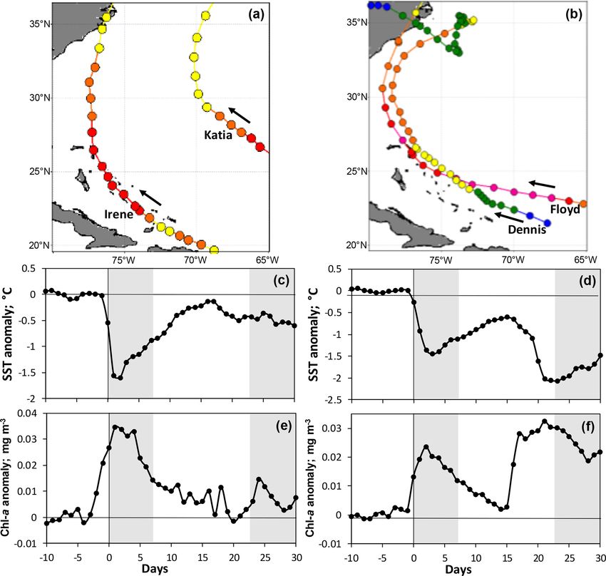
842                               D. Avila-Alonso et al.: Oceanic response to the Hurricanes Dorian and Humberto (2019)

trajectory, which affected this area as a category 3 hurricane     (40 and 45 m along the trajectory and in the square, respec-
(Fig. 1a) a week before the passage of Jerry.                      tively, Fig. 5d).
   When analysing the daily evolution of SST anomalies,
we found that both along the trajectory and in the square
                                                                   3.1.3   Climatological analysis of sea surface
study area SST started to decrease 3 d before Dorian’s ar-
                                                                           temperature
rival, reaching a maximum cooling of approximately 1 ◦ C
about 1 to 3 d after its passage (Fig. 3a). The storm-induced
subsurface thermal variability (described by OHC and T100 )        In order to assess the magnitude of the physical and biologi-
changed in phase with SST (Fig. 3), though OHC and T100            cal response induced by Dorian and Humberto in the square
differed significantly (Mann–Whitney test, p < 0.05) be-           study area, we compared the mean SST and chl a concentra-
tween the studied areas (Fig. 3b and c). More specifically,        tion during the third and fourth post-storm weeks of Dorian
OHC and T100 values were 11 % and 2 % smaller (more neg-           with the climatological records. The actual third and fourth
ative) along Dorian’s trajectory compared with the square          post-storm weeks of Dorian in this area were the ones of 19–
study area during the first post-storm week (Fig. 3b and c).       26 September 2019 and 27 September–4 October 2019, re-
Then, during the third and fourth post-storm weeks SST,            spectively; thus, we assessed the SST and chl a concentra-
OHC, and T100 decreased, with the lowest anomalies in the          tion variability during these weeks in the previous years for
square study area (Fig. 3). In general, SST, OHC, and T100         which satellite observations were available, i.e. 1982–2018
anomalies were then 34 %, 28 %, and 42 % lower in this area        for SST and 1998–2018 for chl a concentration. We refer
than along Dorian’s trajectory. Furthermore, we found that         to these weeks as the third and fourth post-storm weeks of
during the first–second and third–fourth post-storm weeks          Dorian, regardless of the analysed year, and to indicate the
45 % and 90 % of SST anomalies in the square study area ac-        actual oceanic response induced by Dorian and Humberto
counted for a surface cooling of more than 1 ◦ C, respectively,    we specified this was the one in 2019. We computed weekly
while 4 % and 47 % of SST anomalies accounted for a sur-           and corresponding long-term arithmetic means (i.e. clima-
face cooling of more than 2 ◦ C, respectively (Fig. 4). Overall,   tologies) for each variable within the square study area, while
SST, OHC, and T100 anomalies in the square study area were         standardized anomalies (deviations from the climatological
50 %, 63 %, and 57 %, respectively, lower in the third–fourth      weekly mean) were calculated by subtracting the long-term
post-storm weeks than in the first–second post-storm weeks.        weekly mean from the weekly mean of each variable. From
                                                                   Fig. 6a we can see that the SST anomaly in the third post-
3.1.2   Drivers of ocean cooling                                   storm week of Dorian in 2019 was the most negative one
                                                                   in the last 14 years, while only 18 % of the analysed years
We found fluctuations of the MLD before, during, and after         showed anomalies lower than the one in 2019 during this
the passage of Dorian with no significant differences between      week. On the other hand, the SST anomaly in the fourth post-
the studied areas when analysing the entire post-storm period      storm week of Dorian in 2019 was the most negative one
(Mann–Whitney test, p > 0.05). The mixed layer started to          in the last 20 years, while only 13 % of the analysed years
deepen 3 d before Dorian’s arrival in both study areas, reach-     showed anomalies lower than the one in 2019 (Fig. 6a).
ing a maximum mean deepening of 10 m along Dorian’s tra-              Despite the confirmed cooling induced by Dorian and
jectory at day 1 and 11 m in the square study area at day 2        Humberto, a positive trend can be observed in the time se-
(Fig. 5a). A second maximum deepening was observed at the          ries of SST anomalies (Fig. 6a), which could bias the results
end of the second post-storm week and the beginning of the         stated above. This positive trend is consistent with the re-
third one (Fig. 5a). On the other hand, D20 fluctuated con-        ported global surface warming and specifically in the north-
siderably during the analysed post-storm period, with signif-      western Atlantic Ocean (Bulgin et al., 2020). In order to com-
icantly different values between the studied areas (Mann–          pare 2019 SST anomalies with the ones in the previous years
Whitney test, p < 0.05). The largest upward displacement           on the same basis, i.e. without the effect of ocean warming
of D20 during the first two post-storm weeks along the tra-        in the region, we removed the linear trend. Thus, we calcu-
jectory (Fig. 5b) was determined by the majority of pixels         lated the least-squares regression line for this time series and
accounting for shoaling of this isotherm (61 % and 56 % of         subtracted the deviations from this line (i.e. the difference
pixels along the trajectory and in the square area, respec-        between the real observed value and the residual one). From
tively, Fig. 5c) since in both areas the net displacement of       Fig. 6b we can see that when removing the positive trend
D20 was similar at this time (Fig. 5d). This spatial pattern       in data, SST anomalies in 2019 were the coldest ones in the
changed during the third and fourth post-storm weeks, with         climatological record except for the ones in 1984 and 1999.
a higher upward displacement of D20 in the square study            In general, SST values in the analysed weeks in 2019 were
area (Fig. 5b), resulting from both the majority of pixels ac-     significantly lower (Mann–Whitney test, p < 0.05) than the
counting for shoaling of this isotherm (60 % and 73 % of pix-      climatological values at this time (Fig. 7a). When assessing
els along the trajectory and in the square area, respectively,     the SST response induced by Dorian and Humberto in a spa-
Fig. 5c) and a higher net displacement of D20 in those pixels      tially explicit way, we observed that, indeed, these TCs led

Nat. Hazards Earth Syst. Sci., 21, 837–859, 2021                                    https://doi.org/10.5194/nhess-21-837-2021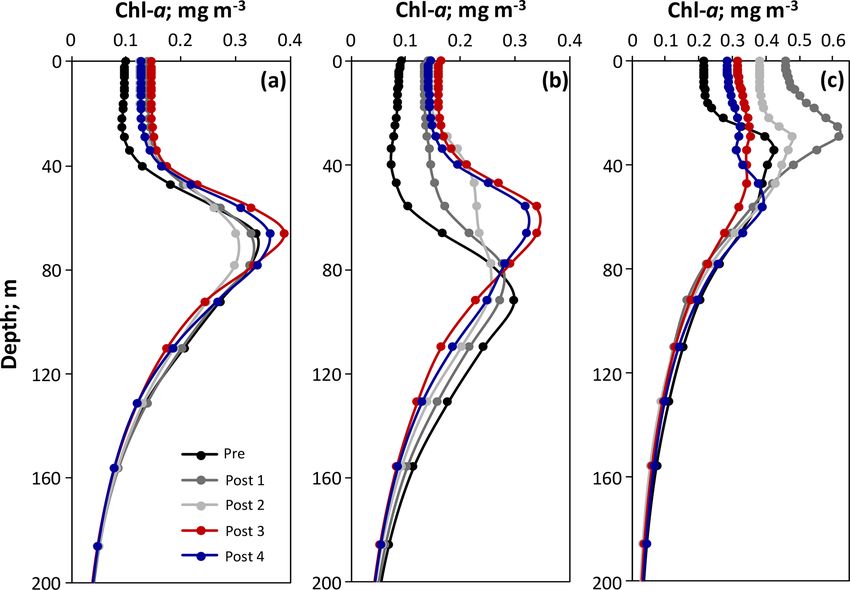
D. Avila-Alonso et al.: Oceanic response to the Hurricanes Dorian and Humberto (2019)                                                   843

Figure 2. Weekly mean sea surface temperature (SST) in the (a) pre-storm week and (b) first, (c) second, (d) third, and (e) fourth post-storm
weeks of Dorian in the Sargasso Sea. The trajectories of Erin and Jerry are superimposed on (a) and (e), respectively, with colour coding as
defined in Fig. 1a and arrows indicating their forward movement. The dashed contours in (b) and (e) indicate the probable surface cooling
induced by Erin and Jerry, respectively.

to a substantial SST cooling over the western Sargasso Sea               being quite distinct from the high-chl a band along the
(Fig. 6c and d).                                                         east coast of USA (delineated by the 0.1 mg m−3 contour in
                                                                         Fig. 8a). Then, following the passage of Dorian, we observed
3.2     Biological response                                              an oceanic chl a increase and also an expansion of the coastal
                                                                         high-chl a band during the entire post-storm period (Fig. 8b–
3.2.1    Chlorophyll a concentration bloom                               e). The oceanic biological response was strongest in the wa-
                                                                         ters to the north and northeast of Grand Bahama, especially
During the pre-storm week of Dorian, the spatially averaged              during the third and fourth post-storm weeks (Fig. 8d and e).
chl a concentration along its trajectory and in the square                  Taking into account the daily evolution of chl a concentra-
study area was 0.074 and 0.049 mg m−3 , respectively, which              tion anomalies, we found that chl a started to increase 3 d
was low compared to climatological records for the period                before Dorian’s arrival (only along its trajectory, Fig. 9a).
1998–2018, i.e. 0.088 and 0.060 mg m−3 , respectively. Over-             Then, chl a peaked at days 2 and 3 along its trajectory and
all, chl a concentration was low and spatially homogeneous               in the square study area, respectively, with anomalies being
in the deep waters of the western Sargasso Sea at this time,             23 % higher in the former area than in the latter one during

https://doi.org/10.5194/nhess-21-837-2021                                          Nat. Hazards Earth Syst. Sci., 21, 837–859, 2021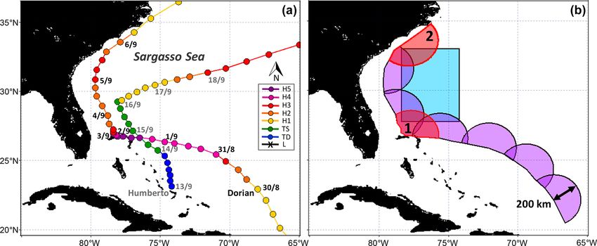
844                                D. Avila-Alonso et al.: Oceanic response to the Hurricanes Dorian and Humberto (2019)

Figure 3. Daily mean evolution of anomalies of (a) sea surface temperature (SST), (b) ocean heat content (OHC), and (c) average temperature
from the sea surface to a depth of 100 m (T100 ) in the Sargasso Sea before, during, and after the passage of Dorian and Humberto. The grey
shaded area depicts the third and fourth post-storm weeks of Dorian which account for the combined effects of Dorian and Humberto.

Figure 4. Sea surface temperature (SST) anomalies in the (a) first–second and (b) third–fourth post-storm weeks of Dorian in the square
study area shown in Fig. 1b.

the first two post-storm weeks. A second chl a maximum                     In order to assess the subsurface biological response, we
was observed at the end of the second post-storm week along             analysed vertical profiles of chl a concentration in the square
the trajectory, while in the square study area, chl a concen-           study area and in semi-discs 1 and 2 (see Fig. 1b) given
tration fluctuated considerably from the end of the second              the high post-storm spatial variability of chl a concentration
post-storm week on but still showing higher anomalies than              profiles along Dorian’s trajectory. Semi-disc 1 was crossed
the ones along the trajectory at this time (Fig. 9a). When              by both studied TCs, while semi-disc 2 was only affected
analysing the frequency of occurrence of chl a concentration            by Dorian. Although the DCM does not always coincide
anomalies in the square study area during the first–second              with biomass or productivity maxima, it often corresponds to
and third–fourth post-storm weeks, we found that 55 % and               peaks in abundance of phytoplankton (reviewed by Moeller
80 % of the anomalies were higher than 0.01 mg m−3 , respec-            et al., 2019). Thus, we considered the chl a concentration
tively, while 36 % and 57 % of the anomalies were higher                in the DCM (chl aDCM ) as a proxy of phytoplankton abun-
than 0.02 mg m−3 , respectively (Fig. 9b and c). Overall, sur-          dance. Figure 10a shows that although the depth of the
face chl a concentration anomalies were 16 % higher in the              DCM (DCMZ ) did not change in the post-storm period, the
third–fourth post-storm weeks than in the first–second post-            mean chl a concentration in the euphotic zone (chl a200 ) and
storm weeks in this area.                                               chl aDCM was 4 % and 16 % higher in the third–fourth post-

Nat. Hazards Earth Syst. Sci., 21, 837–859, 2021                                          https://doi.org/10.5194/nhess-21-837-2021
D. Avila-Alonso et al.: Oceanic response to the Hurricanes Dorian and Humberto (2019)                                                845

Figure 5. Daily mean evolution of anomalies of (a) mixed-layer depth (MLD) and (b) 20 ◦ C isotherm depth (D20) before, during, and after
the passage of Dorian and Humberto in the Sargasso Sea. (c) Percentage of pixels within each study area indicating upwelling in the post-
storm period. From those pixels with upwelling, (d) displays the magnitude of the upward displacement of D20 as a measure of the seasonal
thermocline upwelling. The grey shaded area depicts the third and fourth post-storm weeks of Dorian which account for the combined effects
of Dorian and Humberto.

Figure 6. (a) Time series of weekly mean sea surface temperature (SST) anomalies during the third and fourth post-storm weeks of Dorian in
the square study area shown in Fig. 1b. (b) Detrended time series of SST anomalies. The dashed lines mark anomalies in 2019 for comparison
with the previous years. (c, d) Spatially explicit SST anomalies (Dorian- and Humberto-induced effects (2019) – Climatology, 1982–2018)
in the third and fourth post-storm weeks of Dorian, respectively.

storm weeks than in the first–second post-storm weeks, re-             in the third–fourth post-storm weeks compared to the first–
spectively (Fig. 10a and Table 1). In addition, the chl a pro-         second post-storm weeks in these two areas is consistent with
files in semi-disc 1 showed the highest post-storm variabil-           the maximum deepening of the MLD and shoaling of D20
ity (Fig. 10b). In this area, chl a200 and chl aDCM were 9 %           (Fig. 10a and b and Table 1). In contrast, the chl a profiles
and 16 % higher in the third–fourth post-storm weeks than              in semi-disc 2 evolved differently (Fig. 10c), with chl a200
in the first post-storm week, respectively (Table 1). More-            being 25 % lower in the third–fourth post-storm weeks than
over, DCMZ was shallower in most post-storm weeks com-                 in the first–second post-storm weeks (Fig. 10c and Table 1).
pared to the pre-storm week (Fig. 10b and Table 1), while
in the second post-storm week the DCM could not be dis-
cerned (Fig. 10b). Overall, the strong biological response

https://doi.org/10.5194/nhess-21-837-2021                                        Nat. Hazards Earth Syst. Sci., 21, 837–859, 2021
846 D. Avila-Alonso et al.: Oceanic response to the Hurricanes Dorian and Humberto (2019)
Figure 7. Dorian- and Humberto-induced (a) sea surface temperature (SST) and (b) chlorophyll a (chl a) concentration variability (light
grey) with climatological records (dark grey) during the third and fourth post-storm weeks of Dorian in the square study area shown in
Fig. 1b.
3.2.2 Climatological analysis of surface chlorophyll a
concentration
From Fig. 11a we can infer that the mean chl a concentra-
Table 1. Mean chlorophyll a concentration in the euphotic zone (chl
a200 , mg m−3 ), chl a concentration at the deep chlorophyll maxi-
tion anomaly in the third post-storm week of Dorian in 2019
mum (chl aDCM , mg m−3 ), depth of the DCM (DCMZ , m), mixed- was the highest one in the last 9 years, while only 23 % of
layer depth (MLD, m) and 20 ◦ C isotherm (D20, m) in the square the analysed years showed anomalies higher than the one in
study area, and semi-discs 1 and 2 shown in Fig. 1b during the pre- 2019. On the other hand, the chl a concentration anomaly
and post-storm weeks of Dorian. in the fourth post-storm week in 2019 was only surpassed
by the one in 1999 (Fig. 11a). In general, the chl a concen-
Pre- Post- 1 Post- 2 Post- 3 Post- 4 tration increase induced by the combined effect of Dorian
and Humberto in the square area was significantly higher
Square
(Mann–Whitney test, p < 0.05) than climatological records
chl a200 0.132 0.159 0.149 0.167 0.155 (Fig. 7b). In agreement with the spatial distribution of the
chl aDCM 0.338 0.328 0.301 0.389 0.362 most negative anomalies of SST shown in Fig. 6c, the most
DCMZ 66 66 66 66 66 positive chl a anomalies during the third post-storm week
MLD 14 18 23 36 25 were observed to the north and northeast of Grand Bahama
D20 198 193 193 172 173
(Fig. 11b) affected by the eyewall winds of these TCs. Con-
Semi-disc 1 versely, in the fourth post-storm week positive chl a anoma-
chl a200 0.111 0.148 0.161 0.175 0.164
lies (and negative SST anomalies in Fig. 11c) were more
chl aDCM 0.299 0.276 – 0.339 0.319 evenly spread, although, in general, a considerable response
DCMZ 92 78 – 56 56 occurred in the latitudinal band 25–30◦ N (Fig. 11c).
MLD 15 20 21 32 27
D20 253 223 225 209 211
4 Discussion
Semi-disc 2
chl a200 0.237 0.386 0.322 0.270 0.260 4.1 Ocean cooling and its drivers
chl aDCM 0.426 0.618 0.479 – 0.390
DCMZ 34 29 29 – 56 The extensive surface cooling observed to the right of
MLD 20 17 33 27 30 Dorian’s trajectory (Fig. 2b and c) was also reported by
D20 180 185 177 189 209 Ezer (2020). In addition, this extensive cooling was consis-
tent with the one observed after the passage of Hurricane
Matthew (2016) (which followed a similar trajectory as Do-
rian) and results from the interaction between a hurricane and
the core of the Gulf Stream flow and its associated eddy field
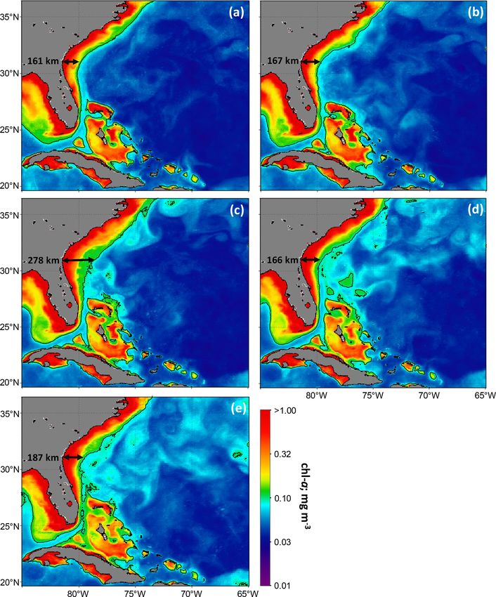
Nat. Hazards Earth Syst. Sci., 21, 837–859, 2021 https://doi.org/10.5194/nhess-21-837-2021D. Avila-Alonso et al.: Oceanic response to the Hurricanes Dorian and Humberto (2019) 847 Figure 8. Weekly mean chlorophyll a (chl a) concentration in the (a) pre-storm week and (b) first, (c) second, (d) third, and (e) fourth post-storm weeks of Dorian in the Sargasso Sea. The contour lines delineate chl a concentration values 0.1 mg m−3 apart. Arrows indicate the distance from the coast to the 0.1 mg m−3 chl a contour. (Ezer, 2018). Dorian induced a disruption of the Gulf Stream imum surface cooling occurred over areas with low values flow, disconnecting the upstream Florida Current from the of sea surface height (SSH) and oceanic cyclonic circulation, downstream of the Gulf Stream and weakening the Gulf which correspond to cold-core eddies (Fig. 12a and c). More Stream flow by almost 50 % (Ezer, 2020). This direct effect specifically, the extensive cooling observed in the centre of on surface currents was followed by intense surface cooling the basin in Fig. 12a largely agrees with the low SSH values largely determined by the reduced flow of warm tropical wa- in it (Fig. 12c). Owing to the special thermodynamic struc- ters being advected downstream of the Gulf Stream as well ture of cyclonic eddies, the MLD within them is relatively as mixing of the upper-oceanic layer (like during Hurricane shallower than in the adjacent ocean, which reinforces the Matthew; Ezer et al., 2017; Ezer, 2020). Overall, the inter- uplifting of cold and nutrient-rich (chl a-rich) subsurface wa- action of hurricanes with the Gulf Stream induces a consid- ters by TC-induced vertical mixing (Ning et al., 2019). This erable vertical mixing and reduction of the stratification fre- also explains the increased chl a concentration to the right of quency (Kourafalou et al., 2016). Consequently, it has been Dorian’s trajectory in regions with oceanic cyclonic circula- reported that vertical mixing drove cooling of the upper 50 m tion (Fig. 12b and c). after the passage of Matthew across the Sargasso Sea (Ezer, The fact that SST anomalies in both study areas are similar 2018). On the other hand, we found that in some cases, max- until day 11 (Fig. 3a) follows from the fact that the centre of https://doi.org/10.5194/nhess-21-837-2021 Nat. Hazards Earth Syst. Sci., 21, 837–859, 2021
848                                D. Avila-Alonso et al.: Oceanic response to the Hurricanes Dorian and Humberto (2019)

Figure 9. Daily mean evolution of (a) chlorophyll a (chl a) concentration anomalies in the western Sargasso Sea before, during, and after
the passage of Dorian and Humberto. The grey shaded area depicts the third and fourth post-storm weeks of Dorian which account for
the combined effects of Dorian and Humberto. Distributions of chl a concentration anomalies in the (b) first–second and (c) third–fourth
post-storm weeks of Dorian in the square area delineated in Fig. 1b.

Figure 10. Spatially averaged chlorophyll a (chl a) concentration profiles in the (a) square study area and the 200 km radius semi-discs (b)
1 and (c) 2 shown in Fig. 1b.

Nat. Hazards Earth Syst. Sci., 21, 837–859, 2021                                          https://doi.org/10.5194/nhess-21-837-2021
D. Avila-Alonso et al.: Oceanic response to the Hurricanes Dorian and Humberto (2019)                                                   849

Figure 11. (a) Time series of weekly mean chlorophyll a (chl a) concentration anomalies during the third and fourth post-storm weeks of
Dorian in the square study area delineated in Fig. 1b. The dashed lines mark anomalies in 2019 for comparison with the previous years.
(b, c) Spatially explicit chl a anomalies (Dorian- and Humberto-induced effects (2019) – Climatology, 1998–2018) in the third and fourth
post-storm weeks of Dorian, respectively.

Figure 12. Oceanic response to Dorian (4 September 2019). (a) Sea surface temperature (SST), (b) chlorophyll a (chl a) concentration,
and (c) absolute sea surface height (SSH) with the absolute geostrophic velocity vectors superimposed (data derived from SSALTO/DUACS
gridded multimission altimeter at 0.25◦ × 0.25◦ spatial resolution). The trajectory of Dorian and a hurricane symbol indicating its estimated
position are superimposed in all imagines.

Dorian moved over the warm waters of the Gulf Stream cur-                ing induced by TCs can extend over vast areas far from the
rent. Despite the Dorian-induced SST decrease in the area,               area affected by the TC centre because of the remotely in-
the warm core of the Gulf Stream (although weakened) was                 duced mixing (Oey et al., 2006, 2007; Vincent et al., 2012a;
still observed most post-storm days (e.g. Figs. 2b and 12a).             Menkes et al., 2016; Ezer, 2018). This contributed to the SST
On the other hand, it has been reported that sea surface cool-           decrease in the square study area and the deepening of the

https://doi.org/10.5194/nhess-21-837-2021                                          Nat. Hazards Earth Syst. Sci., 21, 837–859, 2021
850                                D. Avila-Alonso et al.: Oceanic response to the Hurricanes Dorian and Humberto (2019)

mixed layer 3 d before the arrival of Dorian in both study ar-       the classification of Mignot et al. (2011, 2014). In contrast,
eas (Figs. 3a and 5a). Summer conditions in the Sargasso Sea         in environments with a deep and strong mixing, phytoplank-
are characterized by a strong thermal stratification of the up-      ton are homogeneously distributed in the mixed layer and
per water column, leading to shallow mixed layers (< 20 m            chl a profiles are sigmoid (Mignot et al., 2011, 2014). Given
Michaels et al., 1993; Steinberg et al., 2001). Spatially aver-      the TC-enhanced vertical mixing and deepening of the mixed
aged MLD during the pre-storm week was approximately 14              layer, a shift from Gaussian to sigmoid-like shape of the chl
and 16 m along the trajectory and in the square study area,          a profiles can be expected after the passage of TCs across
respectively. Shallow mixed layers indicate that there is cold       a stratified area (Wu et al., 2007). However, a considerable
water near the surface, so that wind-induced mixing gener-           post-storm change of chlorophyll in the surface mixed layer
ates immediate surface cooling. This agrees with the fact that       occurs when the MLD is deeper than the DCM (Wu et al.,
waters of the western Sargasso Sea have a low resistance to          2007), which explains the Gaussian-shaped profiles after the
TC-induced cooling through mixing (see Fig. 5b in Vincent            passage of Dorian and Humberto (Fig. 10) since MLD was
et al., 2012b).                                                      typically shallower than the DCM (Table 1).
   The retrieved temporal dynamics of the MLD during the                On the other hand, the increased post-storm chl a200
first two post-storm weeks (Fig. 5a) largely agrees with the         (Fig. 10 and Table 1) indicates that subsurface phytoplankton
one reported by Foltz et al. (2015). These authors found             bloom was due to new production resulting from a nutrient
that during and immediately following a cyclone’s passage,           influx into the euphotic layer instead of a vertical chl a re-
the spatially averaged MLD in the Sargasso Sea increases             distribution. This also explains the increased post-storm chl
sharply by 7 m on average, while the positive anomaly                aDCM as well as the shallower DCMZ (Fig. 10 and Table 1).
rapidly diminishes during the subsequent days. Then, after           The formation and persistence of the DCM is governed by
the post-storm shoaling of the MLD, it can oscillate (shoal-         biophysical processes accounting for both bottom-up and
ing and deepening) around the same mean depth (Foltz et al.,         top-down controls (Cullen, 2015; Moeller et al., 2019). How-
2015; Zhang et al., 2016; Prakash et al., 2018). However, this       ever, given that light and nutrient availability are primary
temporal evolution considers the oceanic response to an indi-        factors governing phytoplankton abundance and distribution,
vidual TC. The second maximum deepening observed in our              they have also been recognized as relevant drivers of phy-
study at the beginning of the third post-storm week (Fig. 5a)        toplankton communities in the DCM (Latasa et al., 2016).
agrees with the suggestion made by Ezer et al. (2017), stating       It has been reported that turbulence (like the one induced
that several storms affecting the same region within a rela-         by storms) can enlarge the phytoplankton density above the
tively short period of time have a cumulative impact on ocean        DCM (Liccardo et al., 2013), leading to a shoaling of the
mixing.                                                              DCM. Given that the DCM occurs at the transition between
   For the deep cooling induced by Dorian and Humberto               the light-limited region (below the maximum) and nutrient-
(Fig. 3b and c), we consider this to be largely attributed to up-    limited region (above the maximum), a limited addition of
welling of the thermocline, which explains the more negative         nutrients into the region immediately above the DCM shifts
anomalies of OHC and T100 along the trajectory in the first          the system from a nutrient-limited regime to a light-limited
two post-storm weeks and in the square study area during             one (Liccardo et al., 2013).
the last two post-storm weeks (Fig. 3b and c). TCs typically            Although strong mixing due to TCs is mostly confined to
give rise to upwelling flow underneath the storm centre and          the upper ocean, the cyclone-induced inertial waves affect the
weak downwelling of the displaced warm water over a broad            subsurface mixing too (Prakash et al., 2018). Part of the en-
area beyond the upwelled regions (Price, 1981; Jullien et al.,       ergy transferred to inertial currents by the storm may propa-
2012; Fu et al., 2014). Overall, TC-induced upwelling by Ek-         gate below the mixed layer and finally drive turbulent mixing
man pumping plays a major role in inducing cooling under             in the thermocline (Cuypers et al., 2013). Given that wind-
the TC centre (e.g. Jullien et al., 2012; Wei et al., 2018).         generated inertial waves can propagate up to 2000 m depth
                                                                     in the Sargasso Sea (Morozov and Velarde, 2008), this sub-
4.2   Chlorophyll a concentration bloom                              surface mixing can reach the DCM and nitracline and conse-
                                                                     quently transport chl a and nutrients to the mixed layer (Foltz
The increased post-storm chl a200 and chl aDCM , as well             et al., 2015). The nitracline depth in the northern Sargasso
as the upward displacement of the DCM (Fig. 10 and Ta-               Sea in summer oscillates between 90–150 m (Malone et al.,
ble 1), are consistent with previous observations in several         1993; Goericke and Welschmeyer, 1998), though it decreases
oceanic basins around the world (e.g. Ye et al., 2013; Chacko,       after the passage of TCs (Malone et al., 1993). So, the up-
2017; Chakraborty et al., 2018; Jayaram et al., 2019). A             ward nutrient advection from the nitracline after the passage
DCM typically occurs in stratified and oligotrophic marine           of TCs can fuel subsurface phytoplankton productivity.
environments where phytoplankton are not evenly distributed             For the post-storm surface chl a response, we argue that
throughout the water column (Liccardo et al., 2013; Macías           it was mainly determined by entrainment of chl a from deep
et al., 2013). In this case, the shape of the vertical profiles of   waters given the rapid increase in the surface chl a concen-
chl a concentration can be considered Gaussian according to          tration as soon as a TC reached the study areas, which agrees

Nat. Hazards Earth Syst. Sci., 21, 837–859, 2021                                     https://doi.org/10.5194/nhess-21-837-2021
D. Avila-Alonso et al.: Oceanic response to the Hurricanes Dorian and Humberto (2019) 851
with the suggestion of Shropshire et al. (2016). Figure 12b itude bins (see table in https://www.aoml.noaa.gov/hrd-faq/
shows a patch of high-chl a concentration (0.13 mg m−3 ) to #tropical-cyclone-climatology, last access: May 2020). We
the right of Dorian’s trajectory the day it affected the area, found that Dorian and Humberto had a mean translation
confirming the immediate biological response to the TC forc- speed of 10.95 and 12.8 km h−1 , respectively, in the 25–
ing. Although the mixed layer did not reach the DCM in 30◦ N latitudinal band, while the corresponding mean cli-
the study area (Table 1), it is likely that a small amount of matological translation speed is 20.1 km h−1 . This finding
chl a was eventually transported to the surface since deep agrees with the decreasing TC translation speed observed at
near-inertial mixing can raise the surface chl a concentration global scale in general, and in the North Atlantic basin in
(Wang et al., 2020). The higher chl a concentration anoma- particular, as a consequence of the global-warming-induced
lies along the trajectory compared to the ones in the square changes in global atmospheric circulation (Kossin, 2018;
study area from days −3 to 3 (Fig. 9a) are associated with Lanzante, 2019; Moon et al., 2019; Yamaguchi et al., 2020).
both an increased upward displacement of D20 (Fig. 5b) and Although we acknowledge that pre-storm oceanographic
the horizontal advection of waters rich in chl a from the conditions influence the magnitude of the post-storm oceanic
coast of the northwestern Bahamas and the east coast of the response (Nigam et al., 2019), our climatological analysis re-
USA, which were impacted by Dorian (Avila et al., 2020). vealed that the strongest oceanographic response in the west-
These anomalies of higher chl a concentration are consis- ern Sargasso Sea is associated with consecutive TCs and
tent with the fact that surface phytoplankton blooms are com- long-lasting TC forcing.
mon near the TC trajectory (e.g. Babin et al., 2004; Walker
et al., 2005; Gierach and Subrahmanyam, 2008; Lin and Oey, 4.4 Temporal evolution of the oceanic response to
2016; Avila-Alonso et al., 2019). consecutive TCs
4.3 Climatological analysis of sea surface temperature Climatological SST responses to the passage of TCs in all
and chlorophyll a concentration TC-prone regions around the world indicate that maximum
cooling occurs 2 d after the TC passage, and then cooling
TC activity in the North Atlantic basin peaks from late Au- starts decreasing from this day onward (Menkes et al., 2016).
gust to September (Neely, 2016). Thus, given that the third Moreover, although the TC-induced cold wake in the North
and fourth post-storm weeks of Dorian occurred mainly in Atlantic basin needs about 60 d to disappear, it decays (80 %)
September, the time series of weekly mean anomalies of in the first 20 d (Haakman et al., 2019). On the other hand,
SST and chl a concentration (Figs. 6a and 11a) indicated even though post-storm blooms can last about 2–3 weeks,
the oceanic responses to preceding TCs. For instance, ex- their peak occurs following the passage of TCs (at days 3 to
treme anomalies observed in 1999 (Figs. 6a and 11a) were 4) (Menkes et al., 2016). However, we found that the pas-
associated with the increased oceanic response induced by sage of a second TC disrupts these global patterns, leading
the passage of consecutive Hurricanes Dennis and Floyd at to a decreasing SST trend and a second chl a bloom. It could
the end of August and September 1999 as will be shown in be thought that the oceanic disturbances induced by Dorian
the next section (Fig. 13d and f). Other extreme SST and chl would have limited the impacts from Humberto. The latter
a concentration anomalies were the ones in 1984 and 2005 TC affected the study area approximately 2 weeks after the
(Figs. 6a and 11a) associated with Hurricanes Diana (1984) passage of Dorian; thus, there was a short time period for
and Ophelia (2005). Both hurricanes followed peculiar tra- the ocean to fully recover from the Dorian-induced variabil-
jectories since they made clockwise loops, leading to a pro- ity. It has been reported that the TC-induced oceanic vari-
longed forcing time over the ocean and consequently to a ability can limit the sea surface cooling and deepening of
strong oceanic response (Lawrence and Clark, 1985; Beven the mixed layer induced by a second TC (Baranowski et al.,
and Cobb, 2006). 2014). These authors found a SST decrease of 0.67 ◦ C after
The strong oceanic response to the combined effect of the passage of Typhoon Hagupit, while the second Typhoon
Dorian and Humberto was reinforced by the fact that they Jangmi (passing 7 d after Hagupit) only induced a decrease
were slow-moving TCs. We computed the translation speed of 0.22 ◦ C.
of Dorian and Humberto following the procedure outlined by In order to assess the individual oceanic response induced
Babin et al. (2004) and Gierach and Subrahmanyam (2008) by Humberto and to compare it with the one induced by Do-
using the “best track” observations of time and position from rian, we computed spatially averaged SST and chl a anoma-
the HURDAT2 database of the National Hurricane Center lies in semi-disc 1 since this area was affected for both
(http://www.aoml.noaa.gov/hrd/hurdat/hurdat2.html, last ac- studied TCs (see Fig. 1). We considered the oceanic pre-
cess: May 2020). In order to classify these TCs on the ba- conditions to the passage of Dorian and Humberto (i.e. days
sis of their translation speed, we followed the approach by −10 to −3 before Dorian and Humberto arrived on 2 and 14
Avila-Alonso et al. (2020); i.e. a fast-moving (slow-moving) September, respectively, at semi-disc 1) as a benchmark for
TC has a higher (lower) translation speed than the climato- comparison with its corresponding post-storm weeks as was
logical one computed for Atlantic TCs averaged in 5◦ lat- described in Sect. 2.3. We found that Dorian and Humberto
https://doi.org/10.5194/nhess-21-837-2021 Nat. Hazards Earth Syst. Sci., 21, 837–859, 2021You can also read