Spectral analysis of climate dynamics with operator-theoretic approaches
←
→
Page content transcription
If your browser does not render page correctly, please read the page content below
Spectral analysis of climate dynamics with
                                                 operator-theoretic approaches
                                                 Gary Froyland1 , Dimitrios Giannakis2,* , Benjamin R. Lintner3 , Maxwell Pike3 , and Joanna
                                                 Slawinska4,5

                                                 1 School  of Mathematics and Statistics, University of New South Wales, Sydney NSW 2052, Australia
                                                 2 Department   of Mathematics and Center for Atmosphere Ocean Science, Courant Institute of Mathematical
                                                 Sciences, New York University, New York, NY, USA
arXiv:2104.02902v2 [physics.ao-ph] 28 Jul 2021

                                                 3 Department of Environmental Sciences, Rutgers, The State University of New Jersey, New Brunswick, NJ, USA
                                                 4 Center for Climate Physics, Institute for Basic Science (IBS), Busan, South Korea
                                                 5 Finnish Center for Artificial Intelligence, Department of Computer Science, University of Helsinki, Helsinki, Finland
                                                 * dimitris@cims.nyu.edu

                                                 ABSTRACT

                                                 The Earth’s climate system is a classical example of a multiscale, multiphysics dynamical system with
                                                 an extremely large number of active degrees of freedom, exhibiting variability on scales ranging from
                                                 micrometers and seconds in cloud microphysics, to thousands of kilometers and centuries in ocean
                                                 dynamics. Yet, despite this dynamical complexity, climate dynamics is known to exhibit coherent modes
                                                 of variability. A primary example is the El Niño Southern Oscillation (ENSO), the dominant mode of
                                                 interannual (3–5 yr) variability in the climate system. The objective and robust characterization of this and
                                                 other important phenomena presents a long-standing challenge in Earth system science, the resolution
                                                 of which would lead to improved scientific understanding and prediction of climate dynamics, as well as
                                                 assessment of their impacts on human and natural systems. Here, we show that the spectral theory
                                                 of dynamical systems, combined with techniques from data science, provides an effective means for
                                                 extracting coherent modes of climate variability from high-dimensional model and observational data,
                                                 requiring no frequency prefiltering, but recovering multiple timescales and their interactions. Lifecycle
                                                 composites of ENSO are shown to improve upon results from conventional indices in terms of dynamical
                                                 consistency and physical interpretability. In addition, the role of combination modes between ENSO and
                                                 the annual cycle in ENSO diversity is elucidated.

                                                 Introduction
                                                 Ever since the discovery of phenomena such as ENSO1 and the Madden-Julian Oscillation (MJO)2 , the
                                                 objective identification and characterization of coherent modes of climate variability have been vigorously
                                                 studied across the disciplines of Earth system science. In the face of dynamical complexity and event-
                                                 to-event diversity, the state of large-scale patterns of climate dynamics is typically described through a
                                                 reduced representation provided by climatic indices, constructed using physical understanding and/or
                                                 statistical approaches. For example, ENSO is an oscillation with a broadband periodicity of 2–7 years,
                                                 commonly monitored using so-called Niño indices3 . The latter are defined as spatial and temporal
                                                 averages of sea surface temperature (SST) anomalies over the equatorial Pacific source region of ENSO.
                                                 Such indices are employed for a multitude of diagnostic and prognostic purposes, including lifecycle
                                                 composites4 and prediction skill assessment5 .
                                                     Clearly, the success of these efforts depends strongly on the properties of the indices employed to
                                                 characterize the phenomenon of interest. In general, it is desirable that a climatic index be as objective as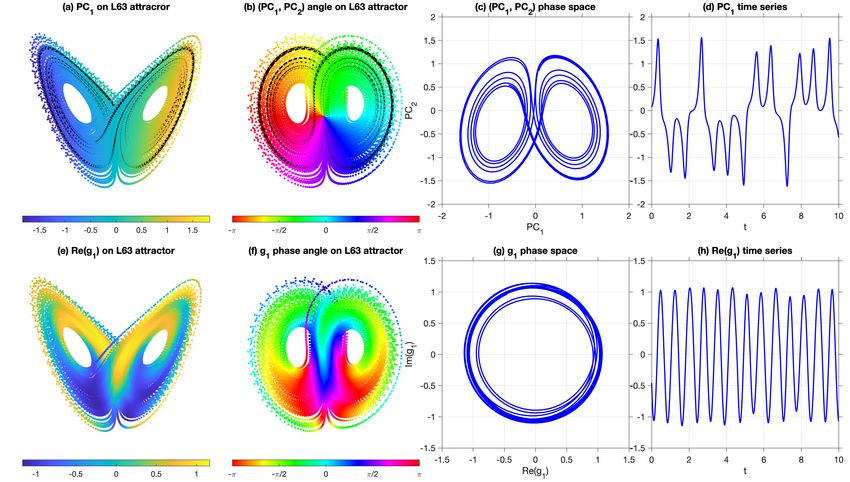
possible, i.e., reveal an intrinsic pattern of climate dynamics independent of subjective choices such as
data prefiltering, or details of the observation modality. For oscillatory patterns such as ENSO and MJO, it
is important that the indices reveal the full cycle as a sequence of observables, e.g., SST fields in the case
of ENSO. Yet, despite their widespread use, conventional approaches for defining climatic indices have
inherent limitations, obfuscating the properties of the phenomenon under study, and sometimes yielding
inconsistent results6 . Empirical Orthogonal Function (EOF) analysis7 , for example, is perhaps the most
commonly used statistical technique for identification of climatic indices, yet it is well known to exhibit
timescale mixing and poor physical interpretability due to EOF invariance under temporal permutations
of the data, even in idealized settings8 . In the context of ENSO, scalar Niño indices do not provide full
information about the state of the cycle because the index could be increasing or decreasing.
    In contrast to EOF analysis and related approaches, which identify patterns based on eigendecompo-
sition of covariance operators, spectral analysis techniques for dynamical systems employ composition
operators, such as Koopman and transfer operators9–11 . A key advantage of this operator-theoretic for-
malism is that it transforms the nonlinear dynamics on phase space to linear dynamics on vector spaces
of functions or distributions, enabling a wide variety of spectral techniques to be employed for coherent
pattern extraction and forecasting. Indeed, starting from early spectral approximation techniques for Koop-
man12, 13 and transfer14–16 operators in the 1990s, there has been vigorous research on operator-theoretic
approaches applicable to broad classes of autonomous17–22 and non-autonomous systems23–28 . In addition,
recently developed methods29–37 combine Koopman and transfer operator theory with kernel methods
for machine learning38–40 to yield data-driven algorithms adept at approximating evolution operators and
their spectra.
    In this paper, we show that the operator-theoretic framework provides an effective route for identifying
slowly decaying (equivalently, slowly decorrelating) observables of the climate system as dominant
eigenfunctions of transfer/Koopman operators and their generator. These eigenfunctions directly describe
coherent climate phenomena such as ENSO, with higher dynamical consistency and physical interpretabil-
ity than indices derived through conventional approaches. The principal distinguishing aspects of this
analysis, illustrated in Fig. 1, can be summarized as:

   1. Identification of cycles from spatio-temporal information: Our spectral approach is based on
      dynamical systems techniques, providing a superior basis for extracting persistent cyclic behavior.
      We transform the underlying full nonlinear dynamics to a larger linear space, yielding a complete
      linear picture for our spectral analysis. This transformation is built directly from physical spatio-
      temporal fields such as SST snapshots. Complex pairs of eigenvalues and their eigenvectors directly
      reveal persistent cycles (see outer panels of Fig. 1) and their periods.

   2. Dynamical rectification: The underlying oscillations in ENSO are clearly revealed in a “rectified”
      two-dimensional (2D) phase space provided by a complex eigenvector. Temporal evolution of the
      oscillation is well described by a harmonic oscillator, represented by motion at a fixed speed around
      a circle in 2D phase space, with the oscillation frequency α determined by the complex eigenvalue.
      Importantly, this property holds true even if the dynamics of the full system is chaotic. See Figs. 2, 4,
      and 5, and accompanying animations in Supplementary Movies 1 and 2 for illustrations. Our
      thorough treatment of rectification clearly shows the asymmetry of ENSO, and enables an estimate
      of the “local speed” of the ENSO cycle.

   3. Phase equivariance: If the 2D phase space is partitioned into S “wedges”, each corresponding to
      a lifecycle phase, then the dynamical evolution of the samples starting in any given phase over a
      time interval of 2π/(Sα) maps them consistently to the next phase. See Fig. 1 (center) and Fig. 9

                                                                                                         2/41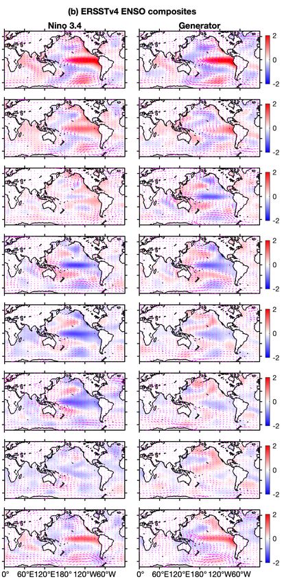
Input spatio-temporal data                    Input spatio-temporal data   Input sp

                                El Nino to La Nina Transition
                                                            Build transfer/Koopman                            Build transfer/Koopman       Build t
                                             Phase 3             operator or generator                         operator or generator.       opera

                    Phase 4                                             Phase
                                                                  Compute       2
                                                                            leading                             Compute leading               Co
                                                              eigenvalues (Figure 3) and                     eigenvalues (Fig. 3) and     eigenva
                                                                    eigenvectors.                                 eigenvectors.                 e

                                                               Provides a projection onto                    Provides a projection onto   Provide
                              Im g

                                                                the dominant cycle and                        the dominant cycle and       the do
Mature La Nina

                                                                                            Mature El Nino
                                                               the cycle frequency. The                      the cycle frequency. The     the cyc
                 Phase 5                                                       Phaseto1
                                                                   cycle is rectified                            cycle is rectified to        cycl
                                                                  proceed at constant                           proceed at constant          proc
                                                                    speed (Figure 5).                              speed (Fig. 5).             spe

                                                                Subdivide the extracted                       Subdivide the extracted      Subdiv
                                                               cycle into phases – see                        cycle into phases – see     cycle i
                                                               Figure 1 (center). These                        Fig. 1 (center). These     Figure
                    Phase 6                                              Phase
                                                                phases are      8
                                                                           equivariant                        phases are equivariant       phase
                                                                and respect the cyclic                        and respect the cyclic       and re
                                                          Re g   dynamics (Figure 9).                            dynamics (Fig. 9).         dyna

                                                                 Produces a cycle of                           Produces a cycle of          Prod
                                                                   spatio-temporal                              spatio-temporal               sp
                                                               composites, e.g. for SST                      composites, e.g. for SST     compo
                                             Phase 7            – see Figure 1 (outer                          – see Fig. 1 (outer         – see
                                                                      panels).                                      panels).
                                La Nina to El Nino Transition
Figure 1. Left: Schematic representation of the canonical ENSO lifecycle recovered from a control
integration of the Community Climate System Model version 4 (CCSM4). Center panel: 2D phase space
associated with the real and imaginary parts of the eigenfunction g of the generator representing ENSO.
Each point in the 2D phase space represents an ENSO state. Dynamical evolution progresses in an
approximately cyclical manner via counter-clockwise rotation. The period of the cycle is equal to
2π/α ≈ 4 yr, where α is the imaginary part of the eigenvalue corresponding to g. The 2D phase space is
partitioned into S = 8 “wedges” of equal angular extent (distinguished by different solid colors), each
corresponding to a distinct ENSO phase. Outer panels: The panels linked to each wedge are phase
composites of SST (colors) and surface wind anomaly fields (green arrows). Collectively, they reveal a
complete ENSO cycle, starting from a mature El Niño in Phase 1, and progressing to an El Niño to La
Niña transition in Phase 3, mature La Niña in Phases 4–5, and La Niña to El Niño transition in Phase 7.
The identified phases are equivariant, meaning that they each span a time interval of 2π/(Sα) ≈ 0.5 yr,
and under forward dynamical evolution by 0.5 yr the samples making up phase i correlate strongly with
the samples making up phase i + 1. By virtue of this property, the generator-based ENSO lifecycle
captures the duration asymmetry between the El Niño to La Niña and La Niña to El Niño transition. This
is evidenced by the fact that the strongest La Niña anomalies occur in Phase 4, as opposed to Phase 5
(which would be expected for a time-symmetric oscillation). Right: Flow chart of the computational
approach for identification of slowly decaying cycles through eigenfunctions of transfer/Koopman
operators. Red-, blue-, and orange-shaded boxes represent input, computation, and output, respectively.

                                                                                                                                   3/41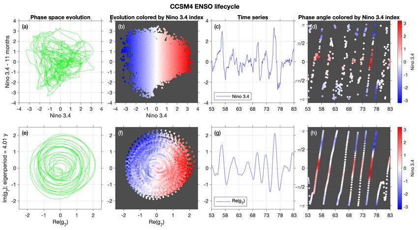
for examples of this behavior with S = 8. An important consequence of equivariance combined
      with slow decay is that it endows the identified phases with higher predictability, while enabling
      the discovery of new mechanistic relationships between physical fields because of a more accurate
      lifecycle. Our improved phasing suggests that ENSO has a more significant cyclical component
      than previously thought.

Results
The perspective adopted here is to view a climatic time series x0 , x1 , . . . , xN−1 ∈ Rd as an observable of
an abstract dynamical system representing the evolution of the Earth’s climate. That is, we envision that
there is an (unobserved) state space Ω and a function X : Ω → Rd such that xn = X(ωn ), where ωn ∈ Ω is
the climate state underlying snapshot xn . Moreover, we consider that there is an (unknown) dynamical
evolution law Φt : Ω → Ω, such that Φt (ω0 ) is the climate state reached at time t starting from an initial
state ω0 . In particular, the climate states underlying the observed data are given by ωn = Φn ∆t (ω0 ), where
∆t is a fixed sampling interval. In the analyses that follow, X will correspond to monthly averaged SST,
sampled at d Indo-Pacific gridpoints at a monthly sampling interval ∆t.
    Given the data xn , our goal is to identify a collection of observables (eigenfunctions) g j : Ω → C with
two main features: cyclicity and slow correlation decay. First, the observables are cyclic in the sense that
there is an associated period over which they approximately return to their original values. Second, the
observables are slowly decaying (or “persistent” or “coherent”) in the sense that their norm decreases
slowly under forward evolution of the dynamics. In the context of this work, “slowly decaying” and
“slowly decorrelating” observables are synonymous notions.
    From a machine learning perspective, this task corresponds to an unsupervised learning problem
aiming to identify slowly decaying cyclic observables. Note that cyclicity is a significantly different
objective than variance maximization performed in the Proper Orthogonal Decomposition (POD), EOF
analysis, and related techniques7, 42, 43 . Complex EOF analysis44 , Principal Oscillation Pattern (POP)
analysis45 and spectral analysis of autoregressive models46 seek to identify oscillatory modes from time
series, though generally through the restrictive lens of linear state space dynamics. Operator-theoretic
approaches are able to consistently extract cyclicity and coherence from nonlinear systems30, 47–49 , without
invoking a specific modeling ansatz such as linear dynamics.
    In the present work, to cope with the high-dimensional data spaces resulting from climatic variables
(e.g., SST fields), these operators will be learned using geometrical kernel methods combined with
delay-embedding methodologies50–52 . Delay-coordinate maps are also leveraged for analysis of climatic
time series by extended EOF (EEOF) analysis53 , Singular Spectrum Analysis (SSA)54–56 , and related
approaches, which extract temporal principal components (PCs) and associated spatiotemporal patterns
(EEOFs) through singular value decomposition of a trajectory data matrix in delay-coordinate space. The
success of these methods at recovering oscillatory patterns, including ENSO, has been interpreted from
both state space56 and operator-theoretic perspectives33, 37 . Ultimately, however, the extracted PCs from
EEOF analysis/SSA are constrained to be linear functions of the delay-embedded data, and do not provide
direct spectral information about evolution operators acting on observables.

Operator-theoretic formalism
Similar to classical methods such as EOF analysis, our approach assumes that the dynamics Φt on Ω is a
stationary, ergodic process. We note that while the climate system is not strictly stationary, our methods
perform well in extracting the dominant cycles on interannual or shorter timescales. Mathematically, the

                                                                                                         4/41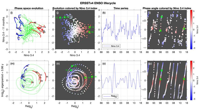
Figure 2. Comparison of EOF analysis (a–d) and transfer operator eigenfunctions (e–h) in extraction of
approximately cyclical observables of the Lorenz 63 (L63)41 chaotic system. Panel (a) shows the principal
component (PC) corresponding to the leading EOF as a scatterplot (color is the EOF value) on the L63
attractor computed from a dataset of 16,000 points along a single L63 trajectory, sampled at an interval of
∆t = 0.01 natural time units. The black line shows a portion of the dynamical trajectory spanning 10 time
units, corresponding to the time series shown in Panels (d, h) and phase portraits in Panels (c, g). Panel (b)
shows the phase angle on the attractor obtained by treating the leading two PCs as the real and imaginary
parts of a complex observable. The black line depicts the same portion of the dynamical trajectory as the
black line in Panel (a). Panel (c) shows a 2D projection associated with the leading two EOF PCs for the
same time interval as Panel (d). Since these PCs correspond to linear projections of the data onto the
corresponding EOFs, the evolution in the 2D phase space spanned by PC1 , PC2 has comparable
complexity to the “raw” L63 dynamics, exhibiting a chaotic mixing of two cycles associated with the two
lobes of the attractor. Panels (e–h) show the corresponding results to Panels (a–d), respectively, obtained
from the leading non-constant eigenfunction g1 of the transfer operator Pε (see Methods). Panel (f) shows
the argument of the complex-valued g1 (color is the argument) evaluated at the 16,000 points in the
trajectory. Notice that there is a cyclic “rainbow” of color as one progresses around each individual L63
attractor wing in phase space. Panel (g) plots these same arguments of g1 , now in the complex plane,
demonstrating that the output of g1 lies approximately on the unit circle. Panel (h) shows the real part of
the trajectory in Panel (g) plotted versus time, illustrating approximately simple harmonic motion. Thus,
the second eigenvector g1 of the transfer operator Pε extracts the dominant cyclic behavior of L63 on the
attractor’s wings.

                                                                                                         5/41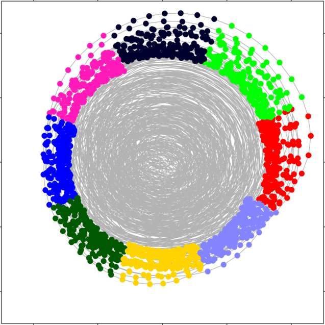
stationarity is governed by a probability measure µ on Ω, which is preserved by the dynamics; formally
µ(Φ−t (A)) = µ(A) for any measurable set A ⊆ Ω. The ergodicity assumption is an indecomposability
hypothesis: there are no non-trivial Φt -invariant sets, meaning that Ω cannot be decomposed into separate
subsystems.
     Operator-theoretic approaches shift attention from studying the properties of the (generally, nonlinear)
flow Φt on state space to studying its induced action on linear spaces of (generally, nonlinear) observables.
We denote by F the space of complex-valued functions on Ω. The space F has the structure of an
infinite-dimensional linear (vector) space equipped with the standard operations of function addition and
scalar multiplication, but the elements    of F need not be linear functions. We will consider the subspace
of observables H = { f ∈ F : Ω | f | dµ < ∞}. Intuitively, thinking of µ as the climatological distribution
                                       2
                                 R

of the system, the space H consists of all observables with finite climatological mean and variance.
     The dynamics acts naturally by composition on each element f0 ∈ H. For invertible Φt , the composition
operator, ft := Pt f0 = f0 ◦ Φ−t , known as the transfer operator, evolves f0 forward t units of time to the
function ft . Dual to (and here, the inverse of) the transfer operator Pt , is the Koopman operator defined by
U t f0 := f0 ◦ Φt . Traveling forward in time along a trajectory {Φt (ω0 )}t≥0 , the observations recorded by
 f0 along this trajectory are f0 (Φt (ω0 )) = (U t f0 )(ω0 ).
     Ergodicity may be equivalently characterized by the constant function 1 being the unique (normalized)
fixed point of U t . Ergodicity implies (via Birkhoff’s Ergodic Theorem or the strong law of large numbers)
that sufficiently long trajectories in Ω will well sample µ. This will be important in this paper because
we are using a single trajectory as our input data. We note that many operator-theoretic algorithms may
also use information from multiple trajectories and are not restricted to using a single time series. Similar
operator constructions can be carried out in other functional settings, notably there is a well-developed
spectral theory for infinite compositions of different transfer operators arising from non-autonomous
dynamical systems24, 57–59 .
     We now describe how the spectral properties of Pt and U t provide natural notions of persistent
almost-cyclic functions and observations. We distinguish between methods applicable for discrete-
and continuous-time dynamics. Discrete-time approaches are based on approximations of the time-1
transfer/Koopman operators, whereas continuous-time approaches target the infinitesimal generators of
the transfer/Koopman evolution semigroups. In the present setting of observables in the Hilbert space H
associated with the invariant measure, the Koopman and transfer operators are unitary, and are duals to
one another under operator adjoints, i.e., Pt∗ = U t . Thus, working with Pt vs. U t is merely a matter of
convention.

Persistent cycles from the spectrum
Discrete time. Let P = P1 be the time-1 transfer operator on H. If Pg = Λg, with g 6≡ 0, we call Λ ∈ C an
eigenvalue and g an eigenfunction. One has11 |Λ| = 1, |g| is constant, and the collection of all eigenvalues
of P, denoted σe (P), is a subgroup of the unit circle (if Λ, Λ̂ ∈ σe (P) then ΛΛ̂ and Λ/Λ̂ are both in σe (P)).
As a simple example, if our phase space is S1 (a circle of circumference 2π) and Φ = Φ1 rotates the circle
by an angle α, then P has eigenvalues Λk = eikα with corresponding eigenfunctions eikθ for k ∈ Z and
θ ∈ S1 . Analogous results hold for the Koopman operator U = U 1 .
    Numerical estimation of P or U inevitably introduces perturbations or “noise” to the operators, and
leads to finite-dimensional representations which cannot exactly comply with the above theory. In
particular, numerical representations of P are often not unitary. Nevertheless, numerical schemes such as
projected restrictions of P or U onto subspaces of H spanned by locally supported or globally supported
basis functions have been highly successful17, 23, 29, 60 and in certain settings, convergence results for
the spectrum and eigenfunctions have been proven14, 15, 22, 61–63 . In these schemes, the spectrum of

                                                                                                          6/41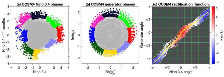
the approximate P is contained in the unit disk {z ∈ C : |z| ≤ 1}, rather than lying on the unit circle
{z ∈ C : |z| = 1}. This addition of noise, which may also be done theoretically, for example by convolution
with a stochastic kernel15, 63, 64 , is frequently harnessed to easily select the most important eigenvalues
from the typically infinite collection σe (P), namely those eigenvalues with large magnitude (close to 1).
    Let Pε denote this perturbed operator and consider an eigenfunction g(ε) corresponding to an eigenvalue
Λ of large magnitude. Because (Pε )t g(ε) = (Λ(ε) )t g(ε) , these eigenfunctions g(ε) decay slowly under
  (ε)

iteration of Pε relative to the decay rates of eigenfunctions corresponding to eigenvalues of smaller
magnitude. It is these “leading” or “dominant” eigenfunctions that will persist over long timescales and
will accurately describe the evolution of the dynamics over similarly long timescales.
    Returning to our example Φ rotating the circle by an angle α, the eigenfunctions of Pε with least decay
will be approximations of (and for carefully chosen approximations, equal to) e±iθ (k = ±1) because they
are the most regular, and persist longest under continued perturbation. The corresponding eigenvalues
       (ε)
are Λ±1 = Rε e±iαε ≈ Rε e±iα , for 0 < Rε / 1, which correspond to rotation by ±α with small decay
rate of Rε per unit time. Thus, the eigenvalues of Pε of greatest magnitude (excluding the eigenvalue 1)
automatically identify the rotation angle α. See Methods for a description of our numerical approach for
approximating P.
Continuous time. In continuous time one can consider generators for the transfer and Koopman
operators. These generators are time-derivatives of Pt and U t , and are given by G f = limt→0 1t (Pt f − f )
and V f = limt→0 1t (U t f − f ), respectively. The operators G and V are defined on a dense subspace of H,
and are skew-symmetric duals to one another, i.e., G = V ∗ = −V . One has σe (G) = σe (V ) are additive
subgroups of iR (the eigenspectrum lies on the imaginary axis in C); that is, if λ , λ̂ ∈ σe (G) = σe (V )
then λ + λ̂ and λ − λ̂ are both in σe (P). Eigenvalues of G and V are interpreted as rates of rotation per
unit time. If our phase space is S1 , and Φt rotates the circle at a rate α, then G and V have eigenvalues
λk = ±ikα and corresponding eigenfunctions eikθ for k ∈ Z and θ ∈ S1 .
    The operators G and V “generate” the semigroup of operators Pt and U t by Pt = etG and U t = etV , and
the spectral mapping theorem connects their spectra: σe (Pt ) = etσe (G) and σe (U t ) = etσe (V ) (if Φt is not
invertible, the spectral value 0 = e−∞ is treated separately). For example, the relationship Λ = eλ links the
eigenvalues Λ of the discrete-time operators with the eigenvalues λ of their continuous-time counterparts.
    As in the discrete-time setting, one may perturb the generators by addition of a diffusion process or
through a numerical scheme. In the former case, if Φt is governed by a vector field then natural “diffused”
versions Gε and Vε of G and V are provided by normalized forward and backward Kolmogorov equations,
respectively. In the latter case, one may apply various numerical schemes26, 30, 34, 36, 65 . The scheme34 is
outlined in the Methods section. The eigenvalues of Gε and Vε are in general complex numbers with zero
or negative real part. For the same reasons as in the discrete-time setting, one seeks eigenvalues with
real part closest to the imaginary axis, which describe the slowest decay rate. In our example of a circle
rotation with rotation rate α, the eigenfunctions of least decay rate are e±iθ (k = ±1) with corresponding
                (ε)
eigenvalues λ±1 = −rε ± iαε ≈ −rε ± iα, for rε / 0 (rε is analogous to log Rε from the discrete-time
setting).

Eigenvalue frequency analysis of monthly-averaged Indo-Pacific SST
We analyze model and observational SST data over the Indo-Pacific domain 28◦ E–70◦ W, 60◦ S–20◦ N.
This domain was selected as a representative region of activity for several large-scale modes of climate
variability on seasonal to decadal timescales, including ENSO, ENSO combination modes66 , and the
Interdecadal Pacific Oscillation (IPO)67 . The model data comprise 1300 yr of monthly-averaged SST fields
from a pre-industrial control integration of the Community Climate System Model Version 4 (CCSM4)68 ,

                                                                                                          7/41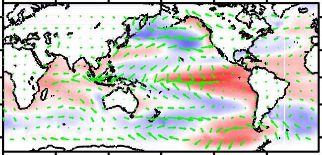
sampled at the model’s native ocean grid of approximately 1◦ resolution. As observational data, we use
monthly averaged SST fields at 2◦ resolution from the Extended Reconstructed Sea Surface Temperature
Version 4 (ERSSTv4) reanalysis product69 over the period January 1970 to February 2020. The resulting
SST data vectors xn have dimension d = 44,771 and 4868 for CCSM4 and ERSSTv4, respectively.
     Our numerical approach builds an approximation of the generator in a data-driven basis consisting
of eigenvectors of a kernel matrix. The kernel matrix, K , has size Ñ × Ñ, where Ñ = N − Q + 1, and is
constructed from delay-embedded SST fields over a window of Q − 1 = 48 lags of length ∆t = 1 month,
corresponding to an interannual time interval of Q ∆t = 4 years. Its eigenvectors represent temporal
patterns that can be thought of as nonlinear generalizations of the PCs obtained via EEOF analysis.
Previously70–72 , such kernel eigenvectors were shown to successfully recover physically meaningful
modes from monthly averaged SST data in both Indo-Pacific and Antarctic domains. For our purposes,
however, the eigenvectors and eigenvalues of K are employed to construct a data-driven version of the
regularized generator Vε , and extract dominant modes by solution of an associated eigenvalue problem
(see Methods). The approximation basis formed by the eigenvectors of K is (i) learned from the high-
dimensional SST data at a feasible computational cost; (ii) is refinable, in the sense of having a well-defined
asymptotic limit as the amount of data N increases; and (iii) as the delay window Q ∆t increases, it is
provably well-adapted to representing eigenfunctions of the generator33, 37 . The results we obtain are not
particularly sensitive to the precise choice of kernels and lags, nor to the use of the generator or transfer
operator. For example, similar results can be obtained with the transfer operator P∆t constructed using
a single lag (Q = 2) of length ` = 12 months (see Methods). A summary of the dataset attributes and
numerical parameters employed in our computations is displayed in Supplementary Table 1.
     Figure 3 and Supplementary Table 2 show eigenvalues λ0 , λ1 , . . . of the generator Vε computed from
the CCSM4 and ERSSTv4 datasets, arranged in order of decreasing real part (i.e., increasing decay rate).
The leading eigenvalues form distinct branches corresponding to (i) the annual cycle and its harmonics;
(ii) ENSO and its combination modes with the annual cycle; and (iii) low-frequency (decadal) modes
with vanishing oscillatory frequency. In the case of the observational data, the spectrum also contains a
trend-like mode representing climate change, as well as combination modes representing the modulation
of the annual cycle by the trend (see Supplementary Fig. 1).
     In interpreting the results in Fig. 3 and Supplementary Table 2, it should be kept in mind that, modulo
a small amount of numerical drift, the CCSM4 data are generated by autonomous dynamics associated
with fixed (pre-industrial) concentrations of greenhouse gases and perfectly periodic radiative forcing
representing the seasonal cycle. In particular, the phase of the seasonal cycle is implicitly represented
in the delay-embedded SST data. The autonomous techniques employed in this paper are therefore
rigorously applicable in this dataset. In contrast, the ERSSTv4 data are subject to different natural
and anthropogenic external forcings (e.g., volcanoes and greenhouse gas emissions, respectively), so
strictly speaking our autonomous methodology does not formally apply here. Nevertheless, our spectral
decomposition separates the trend (corresponding to a real eigenvalue) from the periodic and approximately
periodic cycles (corresponding to complex eigenvalues), which are by definition trendless. In fact, we posit
that an advantage of our approach is that it is capable of extracting trendless cyclical modes in ERSSTv4
without ad hoc detrending of the data, which is oftentimes performed in the context of EOF analysis and
related approaches.
     In both CCSM4 and ERSSTv4, the seasonal-cycle modes occur first in our ordering, which is consistent
with the fact that these are purely periodic modes remaining correlated for arbitrarily long times. Two pairs
of eigenfrequencies ν j := Im λ j /(2π) in this family are accurately identified by the data-driven eigenvalue
problem, namely the annual (1 yr−1 ) and semiannual (2 yr−1 ), eigenfrequencies where the numerical
results agree with the true values to within 1% and 4%, respectively (see Supplementary Table 2). The

                                                                                                         8/41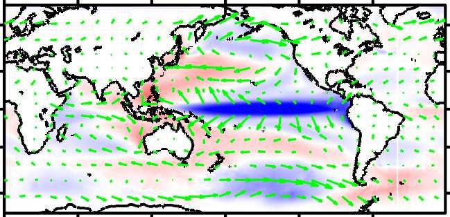
Figure 3. Leading generator eigenvalues λ j computed from (a) CCSM4 and (b) ERSSTv4 Indo-Pacific
SST data, highlighting eigenvalues corresponding to seasonal, interannual, decadal, and trend modes. The
vertical and horizontal axes show the frequency ν j = Im λ j /(2π) and growth rate, Re λ j , respectively.
Note that complex eigenvalues occur in complex-conjugate pairs as appropriate for describing oscillatory
signals at the corresponding eigenfrequencies. Moreover, negative values of Re λ j correspond to decay.
Lines connecting eigenvalues serve as visual guides for the seasonal (periodic), trend, and ENSO branches
of the spectra. The annual (dark blue) and ENSO (red) eigenfrequencies indicated in the spectra
correspond, through their imaginary parts, to the frequencies νannual and νENSO discussed in the main text.
Note that decadal modes are present in the CCSM4 spectrum, but they have larger decay rates, − Re λ j ,
than the range depicted in Panel (a). See Supplementary Table 2 for a listing of the leading 25 generator
eigenvalues extracted from CCSM4 and ERSSTv4.

third (triannual) harmonic is not identified as accurately, being assigned an eigenfrequency of ' 2.5 yr−1
as opposed to the expected 3 yr−1 . This discrepancy is at least partly due to finite-difference errors in our
numerical approximation of the generator; this is discussed in more detail in the Methods section. Other
contributing factors to approximation errors for the eigenfrequencies include the Nyquist limit (which
imposes a limit of 1/(2 ∆t) = 6 cycles/yr on the maximum frequency that can be resolved with a monthly
sampling interval) and the addition of diffusion (which in general perturbs the eigenvalues along both the
real and imaginary axes) in the construction of the regularized generator Vε .
    Beyond the seasonal cycle branch, the CCSM4 spectrum exhibits a branch of eigenvalues consisting of a
pair of fundamental modes with an interannual frequency ν7 ' 0.25 yr−1 =: νENSO , as well as combination
frequencies ν j , j = 9, 11, 13, 15, approximately equal to νENSO + mνannual , where νannual = 1 yr−1 is the
annual-cycle frequency, and m is an integer taking values in the set {−2, −1, 1, 2}. Note that the spacing of
2 in the index j is due to restricting to positive frequencies in this discussion; see Supplementary Table 2.
    We will shortly interpret the eigenfunction corresponding to the eigenvalue νENSO as representing the
fundamental ENSO cycle. We note that this choice is unambiguous as the eigenvalue with largest real part
and frequency close to 0.25 yr−1 . Similarly, the frequencies νENSO + mνannual are naturally interpretable
as combination modes, consistent with the group structure of the generator spectrum described above.
Further notable aspects of these results are that (i) distinct generator eigenvalues correspond to distinct
combination frequencies (as opposed to EOF analysis, which mixes the combination and fundamental

                                                                                                        9/41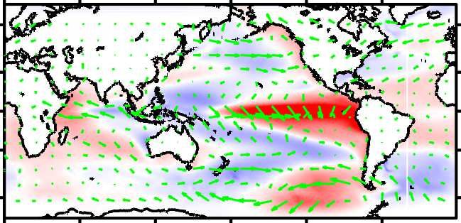
frequencies66 ); and (ii) two harmonics are identified corresponding to the annual and semiannual cycles.
In separate calculations, we have verified that the ENSO eigenfrequencies extracted from the CCSM4 data
remain unchanged to two significant digits for embedding windows ranging from 1 year (Q = 12) to 16
years (Q = 192).
    ENSO and ENSO combination eigenvalues are also identified in the ERSSTv4 spectrum, but these
eigenvalues occur after an eigenvalue with vanishing imaginary part that we interpret as a representation of
climate change trend. As shown in Supplementary Fig. 1(a), the eigenfunction time series corresponding
to this eigenvalue has a manifestly nonstationary character, which is broadly consistent with accepted
climate change signals such as persistent warming from the 1980s to early 2000s, “hiatus” during the
mid to late 2000s, and accelerated warming during the early to mid 2010s73 . In addition, the trend
eigenfunction time series is found to correlate with area-averaged anomalies of Indo-Pacific SST and
global surface air temperature, with 0.83 and 0.78 correlation coefficients, respectively. As with ENSO,
this trend eigenfunction comes with its own “combination frequencies” close to 1 yr−1 (since the trend
frequency is zero), capturing the modulation of the annual cycle by the trend (see Supplementary Fig. 1(b)).
Aside from this trend family, both the CCSM4 and ERSSTv4 spectra contain additional modes with
zero corresponding eigenfrequency, representing internal decadal variability of the Indo-Pacific70, 71 .
The spectra also contain interannual modes with higher frequencies than νENSO , notably a mode with
an approximately 3-year eigenperiod (see Supplementary Table 2). In what follows, we will focus on
the fundamental ENSO eigenfunctions and the corresponding lifecycle analysis. These correspond to
eigenfunctions g7 and g6 in the CCSM4 and ERSSTv4 ordering, respectively. Since the observational data
are sparser and noisier than the model data, we expect larger (numerical) decay rates for the observational
data as stronger diffusion is needed to regularize the generator (see Methods). This is borne out in Fig. 3,
where the real parts of the generator eigenvalues for ENSO and the ENSO combination modes are more
negative for the ERSSTv4 data than for CCSM4.
    In summary, we have extracted ENSO eigenfunctions and eigenfrequencies from two datasets (CCSM4
and ERSSTv4), using two computational techniques (generator and transfer operator) and a range of
numerical parameters (lag and embedding window length). Moreover, in each spectral analysis experiment,
there is no ambiguity in associating particular eigenfunctions with ENSO, as discussed above.

A rectified ENSO lifecycle from eigenfunctions
As described above, when nonzero eigenfrequencies exist, the dominant eigenfunctions correspond to
observables with approximately cyclic evolution, even if the underlying flow Φt is aperiodic. We will use
this idea to extract a rectified ENSO lifecycle from the spatiotemporal SST data.

Factoring out approximate cycles from eigenfunctions. Let (Uε )t g(ε) = (Λ(ε) )t g(ε) as before. We
follow an orbit in state space Ω starting at some ω0 . Evaluating both sides of (Uε )t g(ε) = (Λ(ε) )t g(ε) at
ω0 , we obtain ((Uε )t g(ε) )(ω0 ) ≈ g(ε) (Φt (ω0 )) = (Λ(ε) )t g(ε) (ω0 ), where we have inserted the definition
of U0t as the middle term, recalling we have Uε ≈ U in some sense. Defining the multiplicative action of a
complex number Λ on another complex number by MΛ : C → C by MΛ z = Λz, we have that g(ε) (Φt (ω0 )) ≈
MΛt (ε) (g(ε) (ω0 )). Thus, we may think of the eigenfunction g(ε) as an approximate projection (or factor
map) from Ω to C; this is summarized in the following (approximate) commutative diagram:

                                                       Φt
                                                  Ω            Ω
                                               g(ε)            g(ε)
                                                      Mt (ε)
                                                        Λ
                                                  C            C

                                                                                                          10/41
Evolution under Φt on Ω is projected down (by g(ε) ) to approximately a fixed multiplicative action on
C by Λ(ε) . Further, for |Λ(ε) | ≈ 1, we may consider the multiplicative action of MΛ(ε) as an approximate
(ε)
action on S1 := {z ∈ C : |z| = 1}. Recalling that Λ±1 ≈ Rε e±iα with 0 < Rε / 1, the multiplicative action
(ε)
of MΛ(ε) corresponds to an approximate rotation on S1 by an angle of ±α. Thus, for |Λ±1 | ≈ 1, evolution
±1
under Φt on Ω is projected down (by g(ε) ) to approximately a fixed rotation on S1 by α. The above
statement is illustrated numerically for the Lorenz equations in Fig. 2(e)–(g), where g(ε) (Φt (ω0 )) is plotted
for t ∈ [0, 160]. The evolution lies approximately on S1 ⊂ C (Fig. 2(g)), rotating at an approximately fixed
rate (Fig. 2(h)). See Supplementary Movie 1 for a more direct visualization of these results. Projections of
this type for real eigenfunctions of the transfer operator have been used to project out fast dynamics in
multiple time scale systems74 .
Rectified cycles from eigenfunctions. The fact that the rotation on S1 occurs at close to a fixed rate is
a key aspect of our ENSO analysis, and so we emphasize this property by discussing a simple example
that is strongly illustrative for climate cycles such as ENSO. We imagine a crude model of the ENSO
cycle with one-dimensional phase space Ω = S1 . The dynamics of this idealized model is given by a
flow Φt : S1 → S1 , generated by a nonconstant velocity on S1 . We choose a sawtooth-like velocity field
to model the observation that the La Niña to El Niño transition is slower than the transition in the other
direction75 ; see Fig. 4(c) for the corresponding evolution of a “normalized Niño 3.4” index vs. time and
Supplementary Movie 2 for the corresponding animation. In this situation there is no need to “extract” a
cycle in the dynamics, because the dynamics is a cycle—but importantly with nonconstant speed.
Similar to above, let MΛt denote the flow that advances the angle on S1 by arg(Λ)t, where arg(Λ) =
(2π)/T and T is the period of the cycle. The flow MΛt has a constant velocity around S1 , namely 2π/T ;
see Fig. 4(f) for the corresponding cosine-like evolution. Because Φt and MΛt are both cycles of the
same period, there exists a homeomorphism h : S1 → S1 conjugating Φt and MΛt ; that is, h ◦ Φt = MΛt ◦ h,
summarized in the commutative diagram below:
Φt
S1 S1
h h
MΛt
S1 S1
We denote by θ the angle in the “original” cycle (the upper part of the commutative diagram) and by θ 0
the angle in the rectified cycle (the lower part of the commutative diagram); by definition θ 0 = h(θ ). We
set θ = 0 to represent the peak El Niño state in our crude cyclic model of ENSO, and without loss of
generality we fix h(0) = 0 so that peak El Niño occurs at the same angle θ = θ 0 = 0 in both the original
and rectified cycles. We define θ = π as peak La Niña, according to the original cycle, directly opposing
El Niño; this is represented by the green dot in Fig. 4(a).
0
The eigenfunction of the Koopman operator corresponding to MΛt with eigenvalue Λ is grect (θ 0 ) := eiθ ;
0
this eigenfunction is illustrated Fig. 4(e) where the value of the real part of eiθ is colored. By the
above conjugacy, the function (grect ◦ h)(θ ) = eih(θ ) is an eigenfunction of U t with eigenvalue Λ; see
Fig. 4(a). Because La Niña is reached more quickly from El Niño than vice-versa in the original flow, so
too (by conjugacy) must this occur in the rectified, constant-speed flow. Thus, La Niña in fact appears
earlier than half-way through the rectified cycle; see the green dot in Fig. 4(e), which lies at the angle
h(π). Finally, let forig (θ ) := eiθ represent the complex-valued function corresponding to our crude cyclic
model of ENSO, where θ = 0 is El Niño and θ = π is La Niña. We can map forig to the rectified space
−1 0
by forig ◦ h−1 (θ 0 ) = eih (θ ) ; the real part of this latter function is shown in Fig. 4(b). We will use
11/41Figure 4. Rectification of a variable-speed oscillator by eigenfunctions of the generator. The dynamics is
chosen such that the speed dθ dt is faster when θ lies in the interval Θfast := (0, π) and slower for
θ ∈ Θslow := (π, 2π), resulting in the time series for cos(θ (t)) shown in Panel (c). Panel (a) shows the
state space of the original oscillator, i.e., the unit circle S1 consisting of all phase angles θ ∈ [0, 2π),
colored by the value of the real part of the function forig (θ ) = eiθ , namely Re forig (θ ) = cos θ . In an
analogy with ENSO, θ = 0 and π (green dot) would correspond to El Niño and La Niña climate states,
respectively, while cos θ would correspond to a Niño index. The asymmetry in rotation speed then mimics
the fact that El Niño–La Niña transitions take a shorter amount of time than La Niña–El Niño transitions.
In Panel (d) we push down to rectified state space and show in color the real part of forig ◦ h−1 . Note that
La Niña (green dot) appears earlier in this constant-speed cycle on rectified space; this compensates for
the variations of speed of the original oscillator. It is this representation, i.e., the original “ENSO index”
mapped to the rectified state space, that we focus on in Fig. 5. Panel (e) shows the real part of the
0
eigenfunction grect (θ 0 ) = eiθ (color) on rectified space, which appears as a pure cosine wave in Panel (f).
The evolution of the phase angle in the rectified state space is that of a harmonic oscillator with constant
angular frequency 2π/T ; note the period is T = 4 years in analogy with ENSO. Finally, in Panel (b) we
pull the function grect back to the original space and display the real part of grect ◦ h (color).
12/41versions of the functions forig and forig ◦ h−1 as our main demonstration of our rectification process in
Fig. 5. These results are an example of the automatic rectification performed by Koopman eigenfunctions
(Theorem 17.1111 ) for systems with discrete spectra. Operator-theoretic approaches to different kinds of
rectification have also been explored76, 77 .
Comparing our rectified ENSO eigenfunction lifecycle to the Niño 3.4 index. We now apply the
ideas from the previous two subsections to the CCSM4 and ERSSTv4 data, where grect in those sections
will be the generator eigenfunctions g7 and g6 , arising from these two datasets, respectively. In the
following we will refer to g6 and g7 collectively as simply g j . Figure 5 compares several aspects of
the g j to new, lagged ENSO indices fnino derived from the Niño 3.4 index output from the CCSM4 and
ERSSTv4 data as follows. At each time instance, fnino is a 2D vector consisting of the current Niño 3.4
value and its value ` months in the past; that is, (Niño 3.4(t), Niño 3.4(t − ` months)). We choose ` to
be the lag that gives the most cycle-like behavior for fnino . If the Niño 3.4 index evolved as a perfect
cycle with a period of T = 4` months, the two components of fnino would be in quadrature (90◦ phase
difference), resulting in a purely angular motion in the associated 2D phase space. This situation would be
analogous to the evolution of the forig observable depicted in Fig. 4(a), which is periodic but not of fixed
frequency. Yet, in Fig. 5(a, i), it is evident that the evolution of fnino exhibits significant departures from
an approximate 4-year cycle, featuring both retrograde and radial motion, particularly in the case of the
ERSSTv4 data (Fig. 5(i)). In Fig. 5(d, l), we show the evolution of the phase angle obtained by treating the
components of fnino as the real and imaginary parts of a complex number, analogous to the L63 example in
Fig. 2(b, f) (note that the latter representations are in the full phase space). Here, an approximately cyclical
evolution of fnino would induce an approximately monotonic phase evolution (modulo 2π), which would
additionally be linear for a constant-frequency cycle. While such a behavior is discernible in Fig. 5(d, i),
the phase evolution of fnino is clearly corrupted by high-frequency noise due to retrograde/radial motion.
Consider now the generator eigenfunctions g j . The time series plots (Fig. 5(c, g, k, o)) demonstrate
that the real part of g j is positively correlated with the Niño 3.4 index (the first component of fnino ): large
positive values of Re g j tend to coincide with large positive values of Re fnino , including a number of
significant events in the recent observational record such as the 1997/98 and 2015/16 El Niños. Recall that
despite the presence of a climate-change signal in the ERSSTv4 data, the extracted ENSO eigenfunctions
are trendless. Figure 5(f, n) displays scatterplots of the 2D phase spaces associated with the real and
imaginary parts of g j , colored by the Niño 3.4 index. These plots are analogous to the scatterplots of
Re( forig ◦ h−1 ) in Fig. 4(d), and illustrate that the very negative Niño 3.4 index values (deep blue) occur
not directly opposite the very positive Niño 3.4 index values (deep red), but instead appear earlier in the
rectified cycle. These facts and the fact that the corresponding eigenfrequencies ν j are interannual and
well-approximate νENSO , provide evidence that the g j provide a representation of the ENSO lifecycle; a
fact which will be corroborated further below using phase composites. Before doing that, however, we
note two important aspects of the results in Fig. 5.
First, the generator eigenfunctions provide a significantly more cyclic representation of the ENSO
lifecycle than conventional Niño indices. In Fig. 5(e, m), the 2D phase space trajectories associated with
the real and imaginary parts of g j are seen to undergo a predominantly polar evolution, with little to no
retrograde motion when g j is located sufficiently away from the origin (|g j | & 1). As noted above, this is in
contrast to the retrograde and radial motion seen in the Niño 3.4-based fnino index. Moreover, in separate
calculations we have verified that the generator eigenfunctions g j are also more cyclical than the two-
dimensional fnino indices constructed from the Niño 4, 3, and 1+2 indices. Two-dimensional phase space
representations of the ENSO state with approximately cyclical behavior can also be constructed through
multivariate indices, such as SST and thermocline depth anomalies4 , that reveal recharge–discharge
13/41Figure 5. ENSO lifecycle for CCSM4 (a–h) and ERSSTv4 (i–p), reconstructed using lagged Niño 3.4 indices fnino and the complex eigenfunction g j of the generator. Panels (a, e, i, m) show the evolution of the ENSO state in the 2D phase spaces determined from the Niño- (a, i) and generator-based (e, m) indices. For clarity of visualization, in Panel (a) we show the evolution over a 100-year portion of the 1300-year dataset. Significant historical El Niño and La Niña events are marked in red and blue lines in Panel (m) for reference. Panels (b, j) (resp. (f, n)) show scatterplots of the original (resp. rectified) Niño- and generator-based lifecycle colored by the Niño 3.4 index. These plots are analogous to the original and rectified oscillator plots in Fig. 4(d, e), respectively. Panels (c, g, k, o) show Niño 3.4 time series (c, k) and the real part of g j (g, o), plotted over a 30-year portion of the available data. These time series are analogous to those in Panels (c, f) of Fig. 4, respectively. Panels (d, h, l, p) show phase angles determined from fnino (d, l) and g j (h, p). Note that the slope in (h, p) is approximately constant, consistent with the automatic rectification process, namely that trajectories precess around the origin at a fixed angular speed. This regular rectification from our complex eigenvector is in strong contrast to the irregular angular behavior of the lagged Niño 3.4 index in (d, l). 14/41
processes78 , but these representations are also generally less coherent than those provided by the generator
eigenfunctions.
     Second, the generator eigenfunctions “rectify” the ENSO cycle in a manner analogous to the oscillator
example in Fig. 4. In Fig. 5(h), the phase angle associated with the CCSM4-derived g j undergoes a
near-linear evolution, with some excursions from this behavior occurring. We observe that these deviations
from linear behavior occur when the Niño 3.4 (scalar) index is close to zero (white color in Figs. 5(h,p)).
Mathematically, deviations from cyclic behavior are more likely when |g j | is small, which implies Re g j is
also small, and is in turn consistent with weak ENSO amplitude. Visually, the rectification induced by
g j can be seen in the time series plots in Fig. 5(c, g), where a comparatively uniform El Niño–La Niña
cycling of Re g j (Fig. 5(g)) is contrasted with slow La Niña to El Niño ramp ups followed by rapid El
Niño to La Niña decays in the fnino representation (Fig. 5(c)). In Fig. 6(c), we examine the relationship
between the phase angles associated with fnino and g j through a curve fit of θ 0 := arg g j as a function of
θ := arg fnino (shown in a solid yellow line). The fitted curve provides an estimate of the homeomorphism
function h discussed above in the context of the oscillator example. When θ = π (i.e., during La Niñas
according to the Niño 3.4 index), the fitted θ 0 is less than π, which shows that La Niña events occur earlier
than half-way through the g j cycle, as in Fig. 4.
     A similar general behavior of the phase angle is observed for the ERSSTv4 data (Figs. 5(l, p) and 6(f)),
though as one might expect the results are noisier than for CCSM4. Still, the phase angle progression
associated with g j (Fig. 5(p)) exhibits a significantly more rectified behavior than its fnino counterpart
(Fig. 5(l)), particularly during significant El Niño/La Niña events (highlighted with green star markers).
Interestingly, the generator angle arg g j corresponding to La Niña events following strong El Niños (e.g.,
the 1973/74 and 1999/00 La Niñas in Fig. 5(n)) is close to 90◦ . This is consistent with the fact that strong
consecutive El Niño and La Niña events in the observational record have a tendency to occur one year
apart, corresponding to a quarter of the 4-year ENSO cycle.
     In summary, our spectral analysis extracts a canonical ENSO cycle, and provides rectified coordinates
representing the cycle as an approximately fixed-speed oscillation. In rectified space it is clear that the
representation of the ENSO cycle in terms of Niño indices (SST anomalies) is asymmetric because La
Niña appears earlier (in phase/angle space) around the one-dimensional cycle (see Figs. 5(f) and 5(j)).
Without the rectified representation, it would be difficult to assign a characteristic speed/frequency around
the cycle. This notion of characteristic frequency will be useful below for constructing phase composites,
and should also be useful for constructing reduced models. More broadly, we suggest that rectification
is an important conceptual construction, which should be useful in a wide range of climate dynamics
applications.

ENSO phases and their associated composites
We construct reduced representations of the ENSO lifecycle by partitioning the 2D phase spaces associated
with the generator eigenfunctions and lagged Niño 3.4 index into angular phases, and then study the
properties of associated phase composites of relevant oceanic and atmospheric fields. Figure 6(a, b)
and Fig. 6(d, e) depict the phase space partitions over eight such phases for CCSM4 and ERSSTv4,
respectively. Each phase is constructed from samples at times for which |g j | lies in the top m values
in the corresponding 45◦ radial sector, where m = 200 and 20 for CCSM4 and ERSSTv4, respectively.
Larger magnitude values of the eigenfunction g j occur at times belonging to stronger ENSO cycles, and
because we seek a strong canonical ENSO cycle, we subsample at these times. Mathematically, the phase
composites constructed in this manner can be interpreted as conditional expectations of observables (e.g.,
SST anomaly fields) with respect to a discrete variable π j : Ω → {0, 1, . . . , 8} indexing the eight phases
associated with eigenfunction g j . The inclusion of a “zero” phase nominally is to account for states which

                                                                                                       15/41
are not ENSO-active, consistent with earlier work24, 79 that prioritizes larger values of real eigenfunctions
and equivariant functions; see Methods for further details.
It should be noted that in the eigenfunction-based representation, partitioning the phase space into
phases of uniform angular extent is a natural choice since the evolution is rectified and takes place at an ap-
proximately constant angular frequency. In other words, in the eigenfunction picture in Fig. 6(b,e), phases
of uniform angular extent correspond to phases of uniform temporal duration, in this case approximately
4/8 = 1/2 years. In the case of the Niño 3.4-based representation in Fig. 6(a,d), achieving a well-balanced
partitioning is more challenging due to variable/retrograde angular speed and significant radial motion.
Here, we have opted to employ a uniform partitioning scheme which is common practice with many
cyclical climatic indices, including indices for the MJO and other intraseasonal oscillations80 . We note
that this is already an improvement over a characterization of ENSO phases based on scalar indices, since
such representation cannot distinguish the time tendency (increasing or decreasing) of the oscillation.
In both the Niño 3.4- and eigenfunction-based representations, the phases are numbered such that
Phase 1 corresponds to El Niño, and periodic cycling of the phases from 1 to 8 represents an El Niño
to La Niña to El Niño evolution. Turning back to the Niño-3.4 representation in Fig. 5(b), Phase 5 is a
La Niña phase centered at angle π. On the other hand, in the generator representation in Fig. 5(f), La
Niña (deep blue, corresponding to lowest Niño-3.4 values) occurs at Phase 4, centered at 3π/4, due to the
rectification. This means that the rectified generator representation allocates more phases (Phases 5–8) in
the La Niña to El Niño portion of the ENSO lifecycle, thus yielding a more granular description of ENSO
initiation processes.
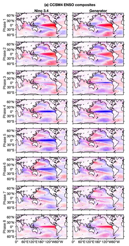
In Fig. 7, we examine phase composites of monthly averaged SST and surface wind anomalies,
constructed using the Niño 3.4 and generator phases from CCSM4 and ERSSTv4 depicted in Fig. 6.
In the the CCSM4 analysis we use surface wind data from the atmospheric component of the model
(CAM2). In the ERSSTv4 analysis, the surface wind data is from the NCEP/NCAR Reanalysis 1 product81 .
First, on a coarse level, both the Niño- and generator-based composites recover the salient features of
the ENSO lifecycle. These include (i) the characteristic El Niño “tongue” of positive SST anomalies in
the Eastern equatorial Pacific, together with its associated anomalous surface westerlies, in Phase 1; (ii)
meridional discharge in the ensuing intermediate phases; and (iii) formation of negative SST anomalies and
easterly surface winds during the La Niña phases (Phases 5 and 4 for the Niño- and eigenfunction–based
representations, respectively).
The Niño-3.4 and generator-based composites in Fig. 7 also exhibit important differences, particularly
in the La Niña to El Niño transition phases. In both CCSM4 and ERSSTv4, Phases 6–8 of the generator
capture a reorganization of the large-scale surface winds from a convergent configuration over the Maritime
Continent in Phase 6 to a divergent configuration initiating in Phase 7 with a buildup of anomalous
westerlies in the Western Pacific, developing further in Phase 8. In particular, the anomalous westerlies in
Phase 7 are consistent with the aggregate effect of higher-frequency, stochastic atmospheric variability
such as westerly wind bursts82 that trigger the development of El Niño events.
To examine this behavior in more detail, in Fig. 8 we show phase-composited zonal wind profiles at the
dateline for the latitude range 40◦ S–40◦ N. These composites recover a number of important atmospheric
features of the ENSO lifecycle, including (i) the mature El Niño state in Phase 1 characterized by strong
westerlies in the tropics maintaining positive SST anomalies in the eastern part of the Pacific basin; (ii)
El Niño decay in Phase 2 with decreasing easterly intensity and a southward shift83 of the anomalous
equatorial westerlies; (iii) La Niña initiation in Phase 3; (iv) La Niña growth, saturation, and decay in
Phases 4–6; (v) El Niño initiation in Phase 7, featuring a clear signal of anomalous westerlies; and (vi) El
Niño growth in Phase 8, cycling back to the mature El Niño state in Phase 1. These features are resolved
in both the CCSM4 and ERSSTv4 datasets, though the observational composites tend to display a higher
16/41You can also read