Local-Scale Carbon Budgets and Mitigation Opportunities for the Northeastern United States
←
→
Page content transcription
If your browser does not render page correctly, please read the page content below
Articles
Local-Scale Carbon Budgets and
Mitigation Opportunities for the
Northeastern United States
Downloaded from https://academic.oup.com/bioscience/article-abstract/62/1/23/295016 by guest on 15 February 2020
Steve M. Raciti, Timothy J. Fahey, R. Quinn Thomas, Peter B. Woodbury, Charles T. Driscoll,
F rederick J. Carranti, David R. Foster, Philip S. Gwyther, Brian R. Hall, Steven P. Hamburg,
J ennifer C. Jenkins, Christopher Neill, Brandon W. Peery, Erin E. Quigley, Ruth Sherman,
Matt A. Vadeboncoeur, David A. Weinstein, and Geoff Wilson
Economic and political realities present challenges for implementing an aggressive climate change abatement program in the United States. A
high-efficiency approach will be essential. In this synthesis, we compare carbon budgets and evaluate the carbon-mitigation potential for nine
counties in the northeastern United States that represent a range of biophysical, demographic, and socioeconomic conditions. Most counties are
net sources of carbon dioxide (CO2) to the atmosphere, with the exception of rural forested counties, in which sequestration in vegetation and
soils exceed emissions. Protecting forests will ensure that the region’s largest CO2 sink does not become a source of emissions. For rural counties,
afforestation, sustainable fuelwood harvest for bioenergy, and utility-scale wind power could provide the largest and most cost-effective mitiga-
tion opportunities among those evaluated. For urban and suburban counties, energy-efficiency measures and energy-saving technologies would
be most cost effective. Through the implementation of locally tailored management and technology options, large reductions in CO2 emissions
could be achieved at relatively low costs.
Keywords: carbon, energy, climate change, land use
D espite overwhelming scientific evidence of the risks
associated with global climate change, limited progress
toward binding global agreements to reduce greenhouse-gas
functions (heating, lighting), and waste disposal. Further-
more, Kuh (2009) argued for the need to design policies
aimed at influencing individual consumer behavior and life-
emissions has been achieved (Bodansky 2010). In the United style, and local governments may be well suited to influence
States, public support for immediate federal government greenhouse-gas-emission behaviors. However, the knowl-
action to address this problem declined between 2006 and edge to most effectively engage local governments in this
2010 (Pew Research Center 2010), and the political climate arena is inadequate (van Staden and Musco 2010), although
in Congress makes near-term climate change abatement leg- some significant initiatives and approaches to address this
islation a remote possibility. Nevertheless, a variety of local limitation have been undertaken (e.g., van Staden and Klas
and regional initiatives, such as the Regional Greenhouse 2010). Economic realities present challenges for financing
Gas Initiative (RGGI; www.rggi.org) and the Western Cli- an aggressive climate change–abatement campaign; there-
mate Initiative (www.westernclimateinitiative.org), have been fore, it is imperative to identify and pursue cost-effective
undertaken in the United States to reduce greenhouse-gas strategies for reducing greenhouse-gas emissions. This task
emissions. Although the feasibility or even desirability of is made more difficult by the complex suite of local and
such fragmentary approaches to climate change mitigation regional factors that influence the abatement potential and
has been questioned (Victor et al. 2005, Wiener 2007), at cost-effectiveness of various mitigation approaches. These
present they are the only game in town. Moreover, cogent factors include biophysical features, such as climate, soils,
arguments, both theoretical and practical, for multilevel topography, and vegetation; demographic factors, such as
governance on this issue have been made (e.g., Trisolini population density and distribution; features of the exist-
2010). For example, local governance plays a key role in a ing infrastructure, including transportation networks, heat
variety of economic activities that significantly influence and power supplies, housing, commerce, and industry;
greenhouse-gas emissions: building codes, zoning regula- and the governance structures in which policies must be
tions, property taxes, public transportation, proprietary positioned.
BioScience 62: 23–38. ISSN 0006-3568, electronic ISSN 1525-3244. © 2012 by American Institute of Biological Sciences. All rights reserved. Request
permission to photocopy or reproduce article content at the University of California Press’s Rights and Permissions Web site at www.ucpressjournals.com/
reprintinfo.asp. doi:10.1525/bio.2012.62.1.7
www.biosciencemag.org January 2012 / Vol. 62 No. 1 • BioScience 23
Articles

   Our objective in this study is to describe how variation
in this suite of factors influences the current carbon balance
(i.e., net carbon dioxide [CO2] fluxes) and the feasibility of
approaches for reducing CO2 emissions in the northeastern
United States. We compare carbon budgets and mitigation
opportunities across nine representative northeastern coun-
ties to illustrate some of the key features influencing the
choice of strategies in this region. We chose the county scale
because it is the smallest political unit for which nationally
consistent data sets related to energy and emissions are
commonly collected (Parshall et al. 2010). We focus on CO2,

                                                                                                                                    Downloaded from https://academic.oup.com/bioscience/article-abstract/62/1/23/295016 by guest on 15 February 2020
which accounts for 77% of anthropogenic greenhouse-gas
emissions (Pachauri and Reisinger 2007) and 85% of US
greenhouse-gas emissions (USEPA 2011a), as the key green-
house-gas involved in the climate change threat. A major
emphasis in our analysis is the contribution of land use to
CO2 emissions, sinks, and mitigation opportunities. Recent
analyses illustrate that land-use options may provide cost-
effective carbon sequestration in the United States
(Lubowski et al. 2006). Although several CO2-emissions
analyses have been conducted at national and global scales        Figure 1. Map of the study area, which includes the states
(Metz et al. 2001, Houghton 2007, USEPA 2011a), few have          participating in the Regional Greenhouse Gas Initiative.
been done at the local scale. We hope that this synthesis         Detailed carbon budgets and mitigation analyses were
stimulates a productive dialogue among policymakers,              conducted for the highlighted counties.
educators, and society at large and offers motivation and
guidance for municipalities who will set goals to decrease
CO2 emissions in response to regional and international           in highly contrasting profiles of energy use, carbon budgets,
initiatives.                                                      and mitigation potential across the region. Six of the coun-
   The region chosen for this study encompasses the states        ties encompass intensive research sites in the National Sci-
involved in the RGGI, an early cap-and-trade system               ence Foundation’s Long Term Ecological Research Network
designed to decrease CO2 emissions from the northeastern          (www.lternet.edu).
United States. Under the RGGI, a cap on CO2 emissions
from the electric power sector has already been applied,          A brief description of our methods
with the goal of a 10% decrease by 2018 (www.rggi.org).           In general, we followed the protocols developed by Vadas
The Northeast region is heavily populated and urbanized           and colleagues (2007) to circumscribe boundary conditions
and currently emits more greenhouse gases than all but five       and to make emissions and sequestration estimates for the
nations: China, Russia, India, Japan, and the United States       counties. Because utility data on heat and power supplies are
(USEIA 2009). Within this region, we chose eight counties,        not generally available at the county scale, we adjusted state-
plus the independent city of Baltimore, for detailed study        level data on the basis of population, employment, housing
(figure 1). Baltimore is the third-largest city (by population    statistics, and typical energy-usage profiles for each housing
and land area) in the region, although it is substantially        type (Vadas et al. 2007). For residential electricity emis-
smaller than New York City (the largest) and may not rep-         sions, for example, we assigned total state-level emissions
resent the most densely populated areas of that city (e.g.,       to the counties in weighted proportion both to the number
Manhattan). Metropolitan areas outside of major cities            of housing units in each county and to the relative energy
are represented by Essex and Middlesex Counties (Boston           usage of the housing types in each county (e.g., the propor-
metropolitan area) and Baltimore County (Baltimore–               tion of single-family detached or single-family attached
Washington metropolitan area). Worcester County, Massa-           homes). Electricity emissions for the residential sector were
chusetts, contains the medium-sized city of Worcester. The        obtained from the US Energy Information Administration’s
four remaining counties do not contain any cities with a          (USEIA) state-level data (USEIA 2010). Relative energy
population of more than 50,000 people. Hereafter, the eight       usage for each housing type was obtained from the USEIA
counties and the independent city of Baltimore will all be        Residential Energy Consumption Survey (USEIA 2005).
referred to as counties. These counties exhibit a wide range      The number and types of housing units in each county were
of demographic and land-use characteristics from highly           obtained from the US Census Bureau (2011). Our analysis
urbanized to heavily forested (table 1). They also encompass      excludes CO2 emissions from air travel and indirect CO2
a moderate range of climatic variation and biotic produc-         emissions associated with the manufacture of imported
tion potential. Together, these factors were expected to result   goods and with the extraction and transport of fossil fuels,

24 BioScience • January 2012 / Vol. 62 No. 1                                                               www.biosciencemag.org
Articles
Table 1. Demographic and land-use information for the eight selected counties and Baltimore City.
Population Heating degree- Cooling degree- Percentage land use†
Area density (people days (base 18.3° days (base 18.3°
County (km2) Population per km2) Celsius) Celsius) Forest Agriculture Developed
Coos, NH 4740 33,111 7 7500 440 87 6 3
Grafton, NH 4532 81,743 18 7500 440 87 6 4
Tompkins, NY 1273 96,500 76 6800 550 43 31 7
Chittenden, VT 1605 146,571 91 7700 490 73 14 13
Worcester, MA 4090 750,963 184 6800 370 68 9 17
Baltimore County, MD 1573 786,547 501 4700 1220 34 37 24
Downloaded from https://academic.oup.com/bioscience/article-abstract/62/1/23/295016 by guest on 15 February 2020
Essex, MA 1297 735,959 567 6400 560 44 8 37
Middlesex, MA 2133 1,467,016 688 6400 550 46 8 42
Baltimore City, MD 207 639,493 3055 4700 1220 8 2 87
†
Land uses not shown include water, bare ground, wetlands, and nonforest vegetation.
km2, square kilometers.
which would be challenging to incorporate without violat- crops (switchgrass and willow for electricity generation,
ing our county-level boundary conditions (designed to pre- soybeans for biodiesel, corn for ethanol); (7) afforestation;
vent double counting of CO2 emissions across geographic (8) residential, commercial, and industrial photovoltaics;
areas); we consider some implications of this approach (9) transportation (for Tompkins County only, including
for informing national policy in a later section discussing increasing personal-vehicle fuel efficiency to 35 and 50 miles
wider applications and implications. For land areas classi- per gallon [mpg], increased bus ridership and carpooling
fied as forested by the US Department of Agriculture Forest to work, traffic signal upgrades, hybrid electric buses, waste
Service, Forest Inventory and Analysis (FIA) data (http:// oil as fuel, production and use of ethanol and biodiesel);
fia.fs.fed.us) were used to estimate changes in forest carbon and (10) combined heating and power (CHP). Near-future
stocks, except for Baltimore City and Baltimore County, technologies, including carbon capture and storage, high-
where more detailed forest and nonforest biomass data were efficiency solar photovoltaics, and fuel-cell vehicles, were
available (Nowak and Crane 2002, Jenkins and Riemann not evaluated. Nuclear power, offshore and small-scale wind
2003). To estimate the potential for carbon sequestration power, and energy efficiency in industrial processes were
by afforestation, we assumed that all inactive agricultural outside of the scope of the analysis. We did not include
land (USDA 2009) is available for afforestation. We used embedded energy (e.g., manufacture, transport, installation
FIA estimates of forest carbon storage for 26–30-year-old of equipment) in our calculations; life cycle assessments of
forest plots in each state (using data from between 2002 solar and wind power indicate that these emissions are small
and 2008) and divided the total biomass by the median relative to their carbon offsets and the total energy generated
age of the forest to provide an estimate of mean annual (Pehnt 2006, Fthenakis et al. 2008). Detailed methods and
sequestration. data sources can be found in Vadas and colleagues (2007),
For the carbon budgets, we used common, widely avail- which we followed in general but with major adjustments;
able data sources when that was possible in order to stan- we describe these adjustments below.
dardize our comparisons across counties and to ensure that
our calculations would be easily repeatable, so that they Solid bioenergy for electricity generation and liquid biofuels for
might serve as a model for calculating carbon budgets and on-road transportation. For bioenergy crops (see box 1)—we
mitigation opportunities for other counties. All of the miti- used a scenario in which solid bioenergy (switchgrass and
gation opportunities evaluated use mature, current tech- willow) would be used in place of coal for electricity gen-
nologies and can be separated into 10 categories: (1) space eration and in which liquid biofuels (ethanol and biodiesel)
and water heating (e.g., improved building insulation, sealed would be used in place of gasoline or diesel in vehicles. All
air leaks, programmable thermostats, lower thermostat scenarios were based on published life-cycle analyses (Ney
temperature settings, boiler maintenance or replacement, and Schnoor 2002 for switchgrass, Keoleian and Volk 2005
geothermal heating); (2) lighting (compact florescent lamps for willow, Wang M 2005 for ethanol, and Sheehan et al.
[CFLs] and LED [light-emitting diode] exit signs); (3) com- 1998 for biodiesel). We used statistical and geospatial meth-
puters and appliances (energy star refrigerators and air- ods to estimate land availability for bioenergy production
conditioning units, and computer energy-saving features); using switchgrass, short-rotation willow, soybeans, and corn
(4) fuelwood harvest for electricity generation; (5) wind without competition with current agricultural production.
power (land-based, utility-scale facilities); (6) bioenergy On the basis of the total area of pasture, hay, and grassland
www.biosciencemag.org January 2012 / Vol. 62 No. 1 • BioScience 25Articles
Box 1. Land cover, albedo, and climate.
The potential climate benefits of carbon sequestration in forests and of replacing fossil fuels with solid biofuels are widely acknowl-
edged. Less appreciated, however, are the concomitant effects of land-use changes on radiative forcing associated with differences in
albedo, evapotranspiration, and surface roughness between native vegetation and bioenergy crops. For example, conversion from
herbaceous vegetation to forest in boreal regions likely has a net warming impact on the climate, whereas similar conversion in broa-
dleaf temperate regions can range from net warming to net cooling (Bala et al. 2007). The differing climate impacts of afforestation in
boreal and temperate forests result especially from the fact that the albedo of deciduous forests is higher than that of evergreen forest,
and that of herbaceous vegetation can be particularly high, especially when the area is snow covered (Bonan 2008). From south to
north across the northeastern United States, forest cover changes from predominantly broadleaf deciduous to evergreen conifer, the
Downloaded from https://academic.oup.com/bioscience/article-abstract/62/1/23/295016 by guest on 15 February 2020
duration of snow cover increases markedly, and the potential yield of biofuel crops and the growth of forests declines. Each of these
differences contributes to the regional variation in the effects of land-use change on radiative forcing. To illustrate the magnitude of
these effects, we compared the climate forcing associated with afforestation and biofuel crops in Baltimore County, Maryland, and
Coos County, New Hampshire (figure 1). We used climate data specific to each location (NCDC 2009), together with albedo estimates
for these land-cover types (Bonan 2008, Jackson et al. 2008) to calculate the annual albedo difference between forest (hardwood or
conifer) and cropland in the two locations. The albedo difference between bioenergy crops and forest is much greater for the northern
location (Coos County; see table 2).
This difference indicates that albedo change has a much greater effect on the climate forcing associated with land-use conversion
to bioenergy crops at northern than at southern locations, even within the relatively restricted Northeast region. In fact, a simple
conversion of the change in albedo to carbon dioxide (CO2) equivalents (see Betts 2000; assuming the change in radiative forcing at
the Earth’s surface is equal to the change in radiative forcing at the tropopause) suggests that the albedo effect of land-use change in
Coos County may greatly exceed the climate forcing associated the effects of bioenergy crops and afforestation on atmospheric CO2
at decadal time scales. In contrast, in Baltimore County, these effects are more comparable. Moreover, the differences in productiv-
ity and carbon sequestration between the northern and southern locations are overshadowed by the contrast in albedo effects. These
observations are meant to illustrate the fact that evaluations of land-use change for climate benefits need to account for forcings other
than carbon sequestration and that these other forcings can vary markedly even within relatively restricted geographic ranges (e.g., the
northeastern United States). A complete quantitative assessment of the climate forcing associated with the land-use change would need
to include surface roughness, evapotranspiration, climate model runs to simulate how radiative forcing at the Earth’s surface influences
radiative forcing at the tropopause (i.e., the layer in the atmosphere at which the radiative forcing by CO2 is determined), and other
factors. Research is needed to better address this important problem.
Table 2. Differences between Baltimore County, Maryland, and Coos County, New Hampshire, for solar radiation,
number of days of snow cover, albedo, and dominant afforestation cover type.
Solar radiation (in megajoules Snow duration Albedo difference between biofuels Afforestation
County per square meter per day) (days) and forest (percentage) cover type
Baltimore County, MD 17.26 13 17.5 deciduous
Coos County, NH 15.29 122 45.5 evergreen
in each county (Homer et al. 2004), we discounted land in our study region. We also used corn yield data from the
federal ownership, land with slopes greater than 15%, and National Agricultural Statistical Service. We developed
land currently in pasture or hay production, determined regression equations to predict corn yield on the basis of
on the basis of the 2007 Census of Agriculture (USDA this index (r 2 = .65; NYSERDA 2011). Assuming a one-to-
2009). We assumed that only 20% of the total available one relationship between grain and stover (Graham et al.
land area would actually be used for bioenergy feedstock 2007), this regression relationship was modified to predict
production. Yield data for dedicated bioenergy feedstocks the aboveground biomass yield of corn, which was used as
are only available from a few locations in the Northeast, a conservative proxy for the potential switchgrass and wil-
and these data are not sufficient by themselves to predict low yield (NYSERDA 2011). This regression equation was
yields across our study region. Therefore, to estimate used to predict switchgrass and willow yield on the land
potential feedstock yields, we used measured crop-yield identified to be potentially available in each county as was
data for all of the counties and an integrated index of soil described above. We performed further regression analyses
and climate characteristics called the National Commodity to quantify the trends from 1960 to 2007 in 35 major crops
Crop Productivity Index (Dobos et al. 2008). This index for each state. For crops with strong evidence of linear
incorporates key soil and climatic characteristics that increases in yield, we predicted the yield increases from
influence crop yields and is available for the locations in 2007 to 2020 and estimated the area of land that would
26 BioScience • January 2012 / Vol. 62 No. 1 www.biosciencemag.orgArticles
become available for each crop for each county. This land f ootage estimates (USEIA 2003) by county population or by
could be available either for increased crop production or student population for educational buildings (US Census
for the production of bioenergy feedstocks. We assumed Bureau 2011). The average electrical, heating, and hot-water
that all of this land could be available for feedstock usage per square foot (USEIA 2003) were used to calculate
production. the annual energy usage for each building type. The fuel
required for each CHP system was estimated using the total
Sustainable fuelwood harvest for electricity generation. Sustain- electrical load and a conservative heat rate (Midwest CHP
able harvest rates from forests were calculated from FIA Application Center 2010). These energy requirements were
data for the years between 2002 and 2008 using the follow- converted to CO2 emissions (USEPA 2011a). The net CO2
ing criteria: (a) The live-forest biomass that accounts for reduction was obtained by summing the current electrical
all types of harvest and removals must be maintained or and thermal CO2 emissions and then subtracting the CO2
Downloaded from https://academic.oup.com/bioscience/article-abstract/62/1/23/295016 by guest on 15 February 2020
increased; (b) at least 35% of logging residue (branches and released from hypothetical CHP systems.
tops) must be left on site, therefore allowing a maximum
of 65% to be removed for feedstock; (c) all dead trees must Light bulb replacement. We assumed a mean total usage of
be left on site; (d) no more than 3% of noncommercial 30 bulb-hours per day for CFL replacement bulbs in an aver-
and commercial standing biomass from trees greater than age housing unit (USEIA 2005).
12.7 centimeters (cm; about 5 inches) in diameter may be
harvested and all residue from these trees must be left on Residential photovoltaics. We assumed that half of all single-
site; and (e) 50% of “other removals” should be added from family dwellings would be realistic candidates for photovol-
the FIA-estimated timber product output. The sum of these taic systems (Anders and Bialek 2006).
criteria provides an estimate of the available biomass that
can be harvested indefinitely (Perlack et al. 2005). Finally, Electric fuel grid mix. For all electricity-based energy savings
an ownership factor of 50% was applied in order to account and new renewable power generation, we assumed that
for the likelihood that only a portion of forest landowners emission reductions would displace emissions from the
would be interested in biomass harvest. In New York State, current mix of fuels in the regional electricity grid (USEPA
this factor has been estimated to range from 10% to 90% 2011b).
(NYSERDA 2011).
Carbon budgets
Commercial-scale wind energy. For this category, we used The counties included in this study span a wide range of
200-meter- (m) resolution simulated wind-resource data population densities, from 7 people per square kilometer
to evaluate the potential for commercial wind power gen- (km2) in Coos County, New Hampshire, to over 3000 people
eration across the counties in New England. Our analy- per km2 in Baltimore City, Maryland. The net CO2 fluxes
sis was focused on terrestrial wind resources. Areas with from the counties were strongly and positively correlated
class 3 (6.4 m per second mean speed at 50 m height) or with population density (figure 2), despite moderate dif-
greater wind power potential were considered commercially ferences in per capita CO2 emissions among the counties
viable sites for wind power generation. Developed areas (figure 3). The current rates of carbon sequestration in veg-
were excluded as potential sites. The information on land etation and soils were inversely related to population density
availability for wind power generation was determined (r 2 = .63); however, this pattern was not robust at the lower
using the 2001 national land-cover database of Homer population densities, because the counties with population
and colleagues (2004). The wind-resource data, obtained densities of less than about 200 people per km2 differed little
from MassGIS (the Massachusetts Office of Geographic from each other in sequestration rates. According to the
Information, Boston), were originally developed by AWS national land-cover database, all counties with population
Truepower (Albany, New York) as part of a project funded densities in this lower range have developed less than 12%
by the Connecticut Clean Energy Fund (now part of of their total land area, and most of that developed area
the Clean Energy Finance and Investment Authority), the falls into the open space and low-intensity development land-
Massachusetts Technology Collaborative, and Northeast use categories (Homer et al. 2004). These data suggest that
Utilities. opportunities for sequestration in vegetation and soils are
not greatly diminished until the developed proportion of the
Combined heating and power. For CHP, we evaluated the landscape exceeds about 10%–15%.
potential CO2-emission reductions that would result if Most of the counties were net sources of CO2 to the
natural-gas-powered CHP systems were installed in all atmosphere, since emissions from fossil-fuel combustion
high-potential buildings in each county: hospitals, edu- exceeded sequestration in vegetation and soils (figure 2).
cational facilities, office buildings, and lodging (hotels, The exceptions were the two most rural, forested counties in
motels, resorts, assisted-care facilities, and dormitories). northern New Hampshire, where the carbon sequestration
The total square footage of each building type in each in growing forests exceeded CO2 emissions. Therefore, much
county was estimated by scaling regional building square of the northeastern United States is a source of atmospheric
www.biosciencemag.org January 2012 / Vol. 62 No. 1 • BioScience 27Articles
additional CO2 will likely decline
unless policies and practices shift
considerably (Hurtt et al. 2002).
Furthermore, sequestration in
northeastern forests is threat-
ened by a number of invasive
pests and pathogens (Lovett et al.
2006) that could significantly
reduce forest biomass over the
coming decades. Finally, forest
cover in the region is declin-
Downloaded from https://academic.oup.com/bioscience/article-abstract/62/1/23/295016 by guest on 15 February 2020
ing as real estate development
expands in both suburban and
rural areas (Stein et al. 2010).
Therefore, if current trends in
land use continue, future car-
bon sequestration potential will
be reduced and some previously
stored carbon in vegetation and
soil will be released to the atmo-
sphere as CO2.
Per capita CO2 emissions
Per capita CO2 emissions among
Figure 2. Net carbon flux plotted against population density. Net-zero emissions, the counties ranged from 2900
where anthropogenic emissions are roughly in balance with sequestration in kilograms (kg) of carbon per
vegetation and soils, coincides with a county population density of about 30 people per person for Chittenden County,
square kilometers (km2; see the inset). Our analysis excludes emissions from air travel Vermont, to 4670 kg of carbon
and indirect emissions associated with the manufacture of imported goods and the per person for Baltimore County,
extraction and transport of fossil fuels. Maryland (figure 3). This range
in per capita emissions is smaller
than international variation
CO2, with the strength of the source varying primarily with (Aldy 2006), but it is still quite large, which suggests that
human population density and with only sparsely populated local factors may exert considerable influence on per capita
forested counties acting as net CO2 sinks. CO2 emissions.
Net-zero emissions of CO2 in the northeastern region The transportation sector accounted for the largest share
coincide with a population density of about 30 people per of CO2 emissions from every county (35%–47%), except
km2, a figure that is based on the regression between net for Baltimore City, Maryland (26%; figure 3). Per capita
CO2 emissions and population density (r 2 = .99; figure 2). transportation CO2 emissions ranged from 920 kg of car-
This value represents the population density at which CO2 bon per person in Baltimore City to 1640 kg of carbon
emissions in the Northeast are roughly in balance with per person in neighboring Baltimore County. The greater
the sequestration in vegetation and soils. Contrast this availability of public transportation and the closer proxim-
value with the mean population density of the region of ity to places of employment play a role in Baltimore City’s
134 people per km2 (US Census Bureau 2011). The implica- lower transportation CO2 emissions. More than 28% of
tion of our results is that sequestration in forests and soils working Baltimore City residents used public transporta-
cannot offset existing emissions from the region. Note that tion, walked, or used alternate means of transportation
our analysis ignores air travel, which constitutes nearly (19.4%, 7.1%, and 1.6%, respectively) to get to work (US
3% of US CO2 emissions (USDOE 2009a), as well as CO2 Census Bureau 2011). Compare these values with those
emissions associated with the production and transporta- for neighboring Baltimore County, where fewer than 8%
tion of imported food and goods, which are at least 10% of working residents used these forms of transportation
of the total emissions for the United States (Davis and for their daily commute. A lower average income com-
Caldeira 2010). bined with more convenient access to public transporta-
The future potential for natural sequestration to offset tion probably contributes to the lower vehicle ownership
regional CO2 emissions is less promising when the patterns rates in Baltimore City, where 30% of households have
of forest regrowth in the Northeast are examined. Forests no personal vehicle (US Census Bureau 2011). The other
in the region are maturing, and their ability to sequester county with comparatively low per capita transportation
28 BioScience • January 2012 / Vol. 62 No. 1 www.biosciencemag.orgArticles
Electricity usage constituted a large and highly variable
percentage of residential CO2 emissions across the coun-
ties and influenced many of the patterns in residential CO2
emissions. Chittenden County, Vermont, has unusually low
per capita residential CO2 emissions because of its extensive
reliance on renewable energy (50%, mostly hydroelectric)
and nuclear power (34%) for electricity generation (VTDPS
2011). These low-carbon-intensity electricity sources result
in residential electricity emissions of only 82 kg of carbon
per person or just 11% of the total residential CO2 emis-
sions. On the other hand, Baltimore City and Baltimore
Downloaded from https://academic.oup.com/bioscience/article-abstract/62/1/23/295016 by guest on 15 February 2020
County had the highest per capita residential electricity use
(0.049 and 0.056 billion British thermal units [Btu] per per-
son, including system losses) and the highest accompanying
CO2 emissions from electricity use, at 750 and 850 kg of
carbon per person, respectively—10 times higher than that
in Chittenden County, Vermont. The warmer climate in
Maryland and the state’s heavy reliance on coal for electric-
Figure 3. Annual per capita carbon dioxide (CO2) emissions ity generation may explain this sharp contrast. Baltimore
for nine northeastern counties in four sectors. The county City averages 1220 cooling degree-days (CDD) per year
population densities increase from left to right. Our versus just 370–560 CDD per year for the other counties
analysis excludes emissions from air travel and indirect (table 1; NCDC 2009), which leads to higher electricity
emissions associated with the manufacture of imported use for home cooling. The milder climate also stimulates
goods and the extraction and transport of fossil fuels. a greater proportion of homeowners to rely on electric
heat, which is a relatively inefficient source; more than 36%
of Maryland residents heat their homes with electricity
CO2 emissions is Tompkins County, New York, which compared with fewer than 10% in the New England states
is dominated by the small city of Ithaca. Ithaca is itself (USEIA 2005).
dominated by Cornell University, which provides strong Fossil-fuel burning for space and hot-water heating
incentives to discourage single-occupancy vehicle com- accounted for the largest proportion of residential CO2
muting. More than 8% of Tompkins County commuters emissions in the upstate New York and New England coun-
use public transportation, and an even greater percentage ties, making up 59%–89% of emissions compared with less
(19.4%) walk or use other alternative means of transit. than 35% of residential emissions in the Maryland coun-
Still, a most-striking pattern is the similarity in per cap- ties. Natural gas and heating oil are favored in the colder
ita transportation CO2 emissions across counties with climate of New England (more than 6000 heating degree-
dramatically different population densities and landcover days [HDD] per year, compared with 4700 HDD per year in
patterns. Baltimore City and County; see table 1).
The residential sector accounted for the second-largest Per capita industrial CO2 emissions were much greater in
share of CO2 emissions in each of the counties (except Bal- Baltimore City and Baltimore County (927 and 1058 mega-
timore City, where it ranked first), accounting for 25%–35% grams [Mg] of carbon per person) than in other counties
of the total CO2 emissions. CO2 emissions ranged from (355–636 Mg carbon per person). Baltimore is home to a
760 kg of carbon per person in Chittenden County, Ver- major port and has historically been a center for industry
mont, to 1260 kg of carbon per person in Coos County, New in the region, despite a major industrial decline in the sec-
Hampshire. Factors such as local climate, housing mix, and ond half of the twentieth century. Finally, the differences
the carbon intensity (the amount of carbon released per unit in per capita CO2 emissions from the commercial sec-
of energy produced) of fuels used for heating and electricity tor are not explained by any obvious factor; for example,
generation contribute to this wide range in residential CO2 the highest and lowest per capita commercial sector CO2
emissions. For instance, Baltimore City has lower per capita emissions were observed in the two northernmost rural
CO2 emissions than Baltimore County, despite similar counties in our study. Detailed study of this variation is
climate and fuel mixes for heating and electricity genera- warranted.
tion. The greater proportion of attached houses, multifamily
dwellings, and apartment buildings in Baltimore City (86% Mitigation opportunities
of housing units) is a major driver of these trends, because The nine counties in this study represent a wide variety of
these smaller, attached housing units require less energy to biophysical, demographic, political, and economic condi-
heat, cool, and light than do detached, single-family houses tions, which in turn influence the feasibility of various
(USEIA 2005). approaches for reducing CO2 emissions. In counties in which
www.biosciencemag.org January 2012 / Vol. 62 No. 1 • BioScience 29Articles
forests and inactive agricultural land are abundant, a variety savings. The actual return on investment may be slower
of land-based strategies offer opportunities to sequester CO2 than is represented here, since the potential interest earned
in vegetation and soils and provide feedstocks for biofuel from alternative investments and the interest paid on loans
production or space to accommodate alternative energy are not considered. However, if CO2 emissions are priced
technologies. In more urbanized counties, in which avail- and energy prices subsequently rise, the return on invest-
able land is limited and expensive, the most cost-effective ment may be faster than we have estimated. Our suite of
carbon-mitigation strategies will include energy-efficiency low-cost mitigation opportunities includes land-intensive
practices and energy-saving technologies. In all cases, a range alternative power sources such as electricity production
of locally tailored management and technology options can from sustainably harvested fuelwood and utility-scale wind
offer substantial CO2-emission reductions at high rates of power. In the residential sector, low-cost opportunities
return on investment, as is described below. include energy-efficient lighting (replacing incandescent
Downloaded from https://academic.oup.com/bioscience/article-abstract/62/1/23/295016 by guest on 15 February 2020
bulbs with CFL bulbs), increased home insulation, pro-
Low-cost mitigation opportunities. We identified and evaluated grammable thermostats, lowered thermostat temperature
a range of low-cost mitigation opportunities (i.e., those settings for heating, sealing air leaks, boiler maintenance
that entail a rapid return on investment; figure 4) that were or replacement, and US Environmental Protection Agency
based on the criterion that they pay for themselves with Energy Star–certified refrigerators and air-conditioning
income generated or through energy-cost savings over the units (Vadas et al. 2007). We focused our analysis on
lifetime of the strategy. For simplicity, we have assumed a the residential sector, together with land-use change and
simple payback period, such that the payback time in years alternative-energy opportunities. Mitigation strategies were
is equal to the initial investment divided by the annual applied to commercial and industrial sectors in cases in which
they were readily transferable and for which supporting data
were available.
Rural counties in our study area (less than 100 people
per km2) could offset 27%–1000% of the current emis-
sions at low cost through the sustainable harvest of fuel-
wood from existing forests and through the installation
of commercial-scale wind-energy farms at favorable sites
(figures 4 and 5). Our wind-energy analysis was focused
on terrestrial wind resources, which are most abundant
in hilly and mountainous terrain; however, the region
also possesses abundant offshore wind resources (figure 5
inset). Because of low population densities, abundant for-
est cover, and favorable topography for wind energy, these
land-based strategies could provide cost-effective reductions
in greenhouse-gas emissions in rural areas. In suburban
counties, these strategies are also favorable (they would,
e.g., reduce emissions up to 116,000 Mg of carbon per
year in Essex County, Massachusetts), although they could
mitigate a smaller proportion of total county CO2 emissions
(0.4%–3.3%).
Regardless of population density and available land
area, the suite of low-cost residential, commercial, and
industrial energy-saving opportunities could be substan-
tial and represent a potential 29%–37% reduction in the
CO2 emissions of the counties in this study. The largest
potential for low-cost residential energy savings was for
space and water heating, for which a combined 9%–13%
reduction in county CO2 emissions could be achieved by
Figure 4. Low-cost mitigation opportunities pay for sealing air leaks, by increasing insulation in older homes,
themselves over time through income generated or energy- by lowering thermostats to 65° Fahrenheit, by using pro-
cost savings over the lifetime of the strategy. The shaded grammable thermostats, through boiler maintenance, and
bars (primary y-axis) show low-cost mitigation potential through the replacement of outdated boilers. Other space-
as a percentage of the current gross county emissions. The and water-heating upgrades would bring even greater
open bars (secondary y-axis) show the absolute mitigation energy savings but would require greater upfront costs.
potential normalized by area. County population densities For instance, augmenting conventional home-heating sys-
increase from left to right. tems with geothermal systems could reduce heating energy
30 BioScience • January 2012 / Vol. 62 No. 1 www.biosciencemag.orgArticles
bulbs. Enabling computer energy-saving features on the
nearly 50% of commercial-sector computers that are cur-
rently set to run constantly (Alliance to Save Energy and
1E 2009) would decrease total county CO2 emissions by
another 1.1%–2.4%.
Combined heating and power, which uses a generator
to produce electrical power while applying the waste heat
for another purpose, is a viable mitigation strategy in all of
the counties. Using waste heat for space heating or absorp-
tion refrigeration can result in energy efficiencies as high
as 85%, compared with 35% for conventional heating and
Downloaded from https://academic.oup.com/bioscience/article-abstract/62/1/23/295016 by guest on 15 February 2020
power systems (Midwest CHP Application Center 2009).
CHP also offers opportunities to switch to lower-carbon
fuels (such as natural gas or biofuels), which can provide
additional reductions in CO2 emissions. The price difference
between electricity and a chosen combustible fuel (typically
less expensive per unit of energy than electricity) is a widely
accepted indicator of the economic feasibility for CHP
systems for a given area (Midwest CHP Application Center
2009). We compared natural gas and electricity prices in the
counties and found that the resulting price differences were
high in all of the counties (between $25.08 and $34.56 per
million Btu), with the exception of Baltimore City and Bal-
timore County, where it was moderate ($12.66 per million
Btu). For buildings in the latter locations to have accept-
able payback periods for CHP systems, other factors would
have to be favorable, such as a good balance of thermal and
electrical load, high heat and electricity demand, or long
Figure 5. The large map shows the percentage of each
operating hours (Midwest CHP Application Center 2009).
county’s undeveloped land area with class 3 (6.4 meters
Our analysis indicates that installing CHP systems in all
per second at 50 meters height) or greater wind potential.
high-potential buildings in each county (hospitals, educa-
The inset map shows the spatial distribution of these
tional facilities, office buildings, and lodging) could reduce
land areas. The information on land availability (i.e.,
CO2 emissions by 0.6%–2.4% (table 3). The use of biofuels
developed or undeveloped) was based on the 2001
as CHP feedstocks could provide even greater CO2-emission
national land-cover database (Homer et al. 2004).
reductions than would the use of natural gas (Eriksson et al.
Our analysis was focused on terrestrial wind resources,
2007).
which are greatest in hilly and mountainous regions,
In total, the low-cost mitigation options that we evaluated
but offshore wind resources are also abundant (see the
could decrease or offset a high proportion of the CO2 emis-
inset map).
sions in the studied counties. For example, the rural coun-
ties that contain small cities, represented here by Tompkins
expenditures by about 50% (USOGT 1998), which would County, New York, (which includes Ithaca) and Chittenden
lead to an 8%–11% reduction in county CO2 emissions. County, Vermont, (which includes Burlington), could offset
Such systems would cost approximately $18,750 for a more than half of their CO2 emissions. At higher population
typical house (Hughes 2008, SBI Energy 2009) and have densities, energy-efficiency strategies and technologies are
a simple payback period of 18–20 years, as determined the most cost-effective options and could offset as much as
from 2008 energy prices in the region. Similarly, residen- 34% of county CO2 emissions.
tial solar hot-water systems (flat plate collectors) could
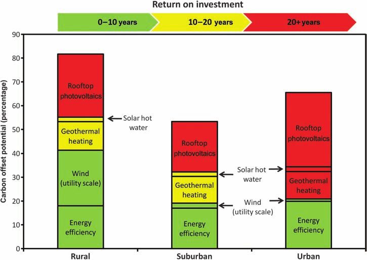
decrease water-heating costs by about 50%, with upfront Higher-cost mitigation opportunities. The higher-cost oppor-
costs of $3250 (USDOE 2010) and a payback period of tunities that we evaluated (figure 8) include terrestrial sinks
14–22 years for a typical home. This could reduce county (e.g., afforestation of inactive agricultural land) and bio-
CO2 emissions by another 1.7%–2.3%. Replacing the 28 energy crops (willow and switchgrass for solid fuels, corn
remaining incandescent light bulbs contained in the aver- ethanol and soybean biodiesel for transportation fuels). We
age home (USDOE 2009b) with more-energy-efficient also evaluated the potential for photovoltaic systems in the
lighting is the next largest low-cost opportunity to reduce residential, commercial, and industrial sectors.
CO2 emissions in the residential sector; county CO2 emis- The rural counties (those with populations under 100 peo-
sions could be reduced by another 2.4%–3.4% with CFL ple per km2) could offset a significant portion of current CO2
www.biosciencemag.org January 2012 / Vol. 62 No. 1 • BioScience 31Articles
Table 3. Potential carbon dioxide (CO2)–emission reductions (megatons of carbon) forests are predicted to be
that would result if natural-gas powered combined heating and power systems were subsumed by urban develop-
installed at all high-potential buildings (hospitals, educational facilities, office buildings, ment between 2000 and 2050
and lodging) in each county. (Nowak and Walton 2005). At
CO2–emissions reduction
present, forest preservation
Educational Office (percentage of gross and afforestation are higher-
County facilities Hospitals buildings Lodging county emissions) cost strategies because of rela-
tively high land values in the
Coos County, NH 129 705 321 994 1.78
region, the low value of car-
Grafton County, NH 1565 1410 1682 1679 1.89
bon offsets in existing markets,
Tompkins County, NY 4699 235 1354 583 2.42 and the challenges of meeting
Downloaded from https://academic.oup.com/bioscience/article-abstract/62/1/23/295016 by guest on 15 February 2020
Chittenden County, VT 2518 235 2503 1371 1.56 additionality and verifiability
Worcester County, MA 7498 3759 8579 2125 0.77 requirements under emerging
Baltimore County, MD 9346 1645 9926 1611 0.61 carbon-accounting frame-
Essex County, MA 6526 4229 8061 2296 0.80 works (Fahey et al. 2010).
Middlesex County, MA 18,365 7989 24,500 4078 1.02
Growing willow and switch-
grass for electric generation
Baltimore City, MD 7484 3994 8314 1234 0.92
could provide relatively large
reductions in CO2 emissions
(table 4) but at a higher price
per unit of energy than coal (Vadas et al. 2007). Cofiring
willow or switchgrass could offset up to 15% of CO2 emis-
sions in rural and suburban counties (up to 75,000 Mg of
carbon per year) without competing with current agricul-
tural production or forestland. Together, afforestation and
bioenergy could offset 0.3%–28% of the CO2 emissions in
rural counties. Afforestation is limited by the availability
of inactive agricultural land, whereas bioenergy feedstocks
are also limited by climate, soil quality, and their proxim-
ity to potential markets or processing facilities (Potter et al.
2007). In the suburban counties (those with fewer than
180 people per km2, excluding Baltimore City), the potential
for afforestation and bioenergy is significant (4700–101,000
and 7600–149,000 Mg of carbon per year, respectively) and
could offset 0.3%–6.8% of current CO2 emissions. However,
it is likely that land prices and development pressure in these
areas will be highest. For instance, Nowak and Walton (2005)
Figure 6. Forest sequestration (light gray) compared with predicted that more than 60% of the land area of four of the
CO2 emissions (dark gray) on a per-area basis for rural most-developed northeastern states (Rhode Island, New
(Articles
Table 4. Summary of the technical potential for switchgrass and forest biofuels, including estimated yields and
carbon offsets.
Switchgrass Fuelwood
Land rent a
Yield (Mg of
b
Offset (Mg
c
Yield (Mg of
(US dollars Crop area carbon per of carbon per Forest carbon per ha Offset (Mg of
County per ha per year) (ha) ha per year) year) area (ha) per year) carbon per year)
Coos County, NH 48 2791 3.8 0 210,707 0.52 104,245
Grafton County, NH 60 623 4.3 0 200,283 0.51 96,747
Tompkins County, NY 47 11,310 9.6 107,840 27,584 0.77 20,054
Chittenden County, VT 59 340 7.6 2584 43,631 0.38 15,695
Downloaded from https://academic.oup.com/bioscience/article-abstract/62/1/23/295016 by guest on 15 February 2020
Worcester County, MA 123 4749 5.2 24,250 134,749 0.48 61,813
Baltimore County, MD 102 20,553 9.2 184,815 22,963 1.25 27,198
Essex County, MA 176 1532 6.5 9822 27,765 1.11 29,171
Middlesex County, MA 178 2546 5.4 13,343 42,076 0.49 19,395
a
Agricultural land rents were not available at the county level. Instead, we estimated county-level land rents based on county-level land prices using the
state-level relationship between land values and agricultural rents for the study states (r 2 = .99). All land-rent and land-value data were from the US
Department of Agriculture (2009).
b
The estimated switchgrass and willow yields for Coos and Grafton counties were too low to be commercially viable (less than 4.5 megagrams [Mg] per
hectare [ha]).
c
Based on substituting biomass for coal in electricity generation.
the application. If the capital costs associated with small- Table 5. Summary of transportation mitigation opportu-
scale photovoltaic systems were to decrease or if the energy nities for Tompkins County, New York.
prices, carbon credits, or efficiency of photovoltaic cells were Carbon offset Percentage
to increase, photovoltaic systems would become a more cost- (megagrams Percentage of total
effective opportunity for the region. Transportation of carbon per of transport gross
mitigation year) emissions emissions
Transportation-sector mitigation opportunities: Tompkins Vehicle fuel efficiency to
20,774 18.90 7.30
County. To illustrate the potential mitigation opportunities 50 mpg
in the transportation sector, we highlight the case of Tomp- Vehicle fuel efficiency to
7226 6.60 2.50
35 mpg
kins County, New York, largely on the basis of the Ithaca-
Tompkins County Transportation Council’s (2004) 2025 Increased carpooling
8200 7.40 2.90
to work
Long Range Transportation Plan. In the plan, the Trans
Increased bus ridership 1417 1.30 0.50
CAD (Caliper Corporation, Newton, Massachusetts) travel-
demand model was used to generate and distribute trips Traffic signal upgrades 670 0.61 0.24
along the road network, which included all state, county, Biodiesel 472 0.43 0.17
and important local roads, and to simulate the results of Ethanol 391 0.35 0.14
proposed transportation upgrades.
Hybrid electric buses 189 0.17 0.07
A broad suite of mitigation opportunities applies to
the transportation sector (table 5), including changes in Waste oil as fuel 73 0.07 0.03
land-development patterns to support mixed-use and Total range †
18,620–32,169 16.9–29.2 6.6–11.3
other environment-friendly zoning practices (Banister
1999). The impact of these land-use-planning activi- †
This range is based on vehicle fuel efficiencies of between 35 miles per
ties was tested with a number of indicators, including gallon (mpg) and 50 mpg.
congestion and vehicle miles traveled. Under proposed
land-use planning scenarios, the model predicted a 2%
decrease in vehicle miles traveled at peak travel times. to work, increasing the use of public transit, upgrading
If this outcome is generalized to include off-peak travel traffic signals, upgrading the county bus fleet to hybrid
times, it would mean a decline of approximately 2% in electric drivetrains, and utilizing in-county waste oil for
county CO2 emissions relative to the business-as-usual fuel (table 5). The opportunity with the largest potential to
scenario. decrease CO2 emissions (of those evaluated) is increasing
Other mitigation opportunities in the transportation passenger-vehicle fuel efficiency. Current passenger-vehicle
sector include improving passenger-vehicle fuel efficiency, fuel efficiency is estimated at 27 mpg, and an increase to
producing transportation biofuels, increasing carpooling 35 mpg would offset transportation-related CO2 emissions
www.biosciencemag.org January 2012 / Vol. 62 No. 1 • BioScience 33Articles
by 6.6%. Increasing effective fuel efficiency to 50 mpg kilowatt-hour) and lowest in Maryland ($0.10–$0.11 per
would lead to a 19% decrease in transportation-related kilowatt-hour). These factors can combine to create dysfunc-
CO2 emissions. The county could provide some incen- tion in the economic incentive structure for carbon abate-
tives to encourage the use of fuel-efficient vehicles, such ment. For example, Baltimore County and City have the
as enhanced parking privileges or special travel lanes for highest carbon intensity for residential heating systems in the
hybrid, plug-in hybrid, and electric vehicles. Increased car- region, yet they have the lowest economic incentive (slowest
pooling could reduce transportation-related CO2 emissions return on investment) for mitigation opportunities (figure 7).
by up to 7.4%, assuming that the majority of people who Clearly, correction of this sort of economic disincentive, such
drive alone to work would participate. Increasing bus rider- as through a rise in the cost of carbon credits under the RGGI,
ship in the county by approximately one third (or 1,000,000 will be needed.
annual rides) would decrease transportation-related CO2
Downloaded from https://academic.oup.com/bioscience/article-abstract/62/1/23/295016 by guest on 15 February 2020
emissions by 1.3%. A mix of smaller upgrades, including Wider applications and implications
traffic-signal upgrades in the city of Ithaca (0.6%), hybrid We chose the county scale as an effective level of analysis
electric buses (0.2%), and using available county waste to inform local policies that could contribute to significant
oil as fuel (0.1%) could further reduce transportation- reductions in greenhouse-gas emissions (e.g., building
related CO2 emissions. These emissions could be offset by and tax codes, public transit, proprietary functions). The
another 0.8% by growing corn and soybeans for ethanol application of analysis at this scale to policy development
and biodiesel, a figure based on a scenario that avoids at larger scales deserves further attention. To avoid double
deforestation and competition with existing agricultural counting, it seemed appropriate to define boundary con-
production. Note that willow, switchgrass, or forest bio- ditions at the county scale; therefore, importation and
fuels could provide larger emission benefits than ethanol cross-boundary transport were not considered, nor were
or biodiesel, especially if they are used in place of carbon- large-scale energy-generation facilities. To inform policies
intensive fuels such as oil (for home heating) or coal (for at the regional and national levels, future development of
electricity generation). Taken in total, these improvements this approach must be embedded in analyses at these larger
have the potential to decrease transportation-sector CO2 scales. The contribution of local analysis to prescriptions
emissions by 17%–29% and total county CO2 emissions for incentives and investments at larger scales also need to
by 6.3%–11% (table 5). The
transportation-related CO2 miti-
gation portfolio for other coun-
ties would vary as a consequence
of differences in current trans-
portation systems and other fac-
tors, but clearly, incentives for
increased passenger-vehicle fuel
efficiency will dominate the miti-
gation opportunities regionwide.
Other patterns in mitigation cost and
potential. A number of regional
and local conditions contribute to
the differences in potential miti-
gation costs and emission benefits
(figure 7) among the counties—
particularly, the mix of fuels used
for heating and electricity gen-
eration, local climate (e.g., cool-
ing and heating degree-days),
and fuel prices. The payback
period for photovoltaic systems;
energy-efficient lighting, air- Figure 7. Return on investment for technological mitigation opportunities for rural
conditioning, and appliances; and (You can also read