THE FATE OF AMPHIBIANS IN AARGAU: EFFECT OF FUTURE LAND-USE SCENARIOS - WSL
←
→
Page content transcription
If your browser does not render page correctly, please read the page content below
Master’s thesis

                  Master’s degree programme in Environmental Sciences

THE FATE OF AMPHIBIANS IN AARGAU:
   EFFECT OF FUTURE LAND-USE
            SCENARIOS
            Identifying Suitable Areas for Blue-Green Infrastructure

                              Lucie Roth (15-929-565)
                         Date of submission: 31 March 2021

Supervisor:        PD Dr. Janine Bolliger
                   Swiss Federal Institute for Forest, Snow and Landscape Research
                   (WSL), Land Change Science
Co-Supervisor:     Dr. Giulia Donati
                   Swiss Federal Institute of Aquatic Science and Technology (Eawag),
                   Urban Water Management
Advisors:          Dr. Peter Bach
                   Swiss Federal Institute of Aquatic Science and Technology (Eawag),
                   Urban Water Management
                   Prof. Dr. Max Maurer
                   Swiss Federal Institute of Aquatic Science and Technology (Eawag),
                   Urban Water Management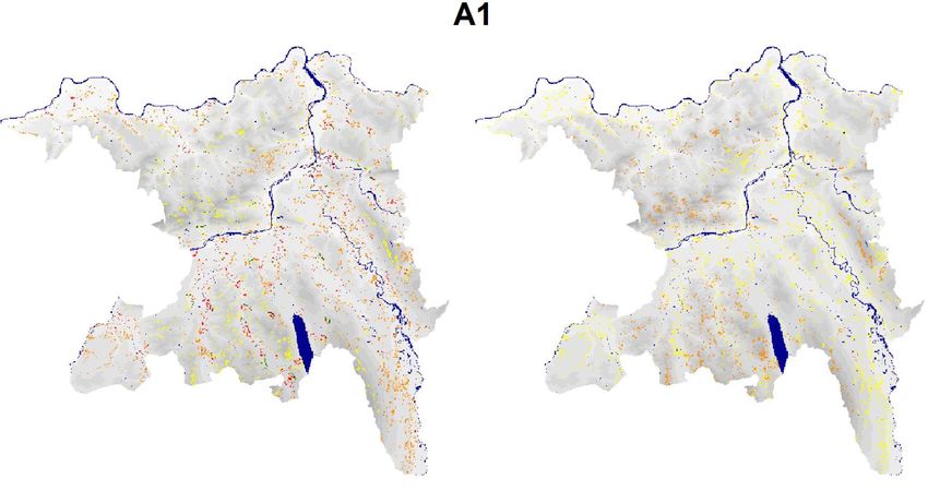
Date:           31 March 2021
Author:         Lucie Roth

Contact:
lucie.roth@usys.ethz.ch / Janine.Bolliger@wsl.ch

ETH Zürich
Department of Environmental Systems Science
Universitätstrasse 16, 8006 Zurich

Proposed citation: Roth, L. (2021): The fate of amphibians in Aargau: effect of future land-
use scenarios. Master’s Thesis ETHZ, D-USYS. Supervisors: PD Dr. J. Bolliger, Dr. G. Donati.

This thesis is part of the project "Blue-green infrastructure for biodiversity enrichment in
human-dominated landscapes". The project belongs to the research initiative "Blue-Green
Biodiversity" (BGB 2020), a collaboration of Eawag and WSL.

The following R-scripts belong to this thesis:
   - 0_Data_Formatting.R (script written by Dr. Giulia Donati)
   - A_Generation_PA_matrix.R
   - B_Environmental_Predictors.R

   - C_biomod2.R
   - D_Output_Analysis_Figures.R

                                                                                          ii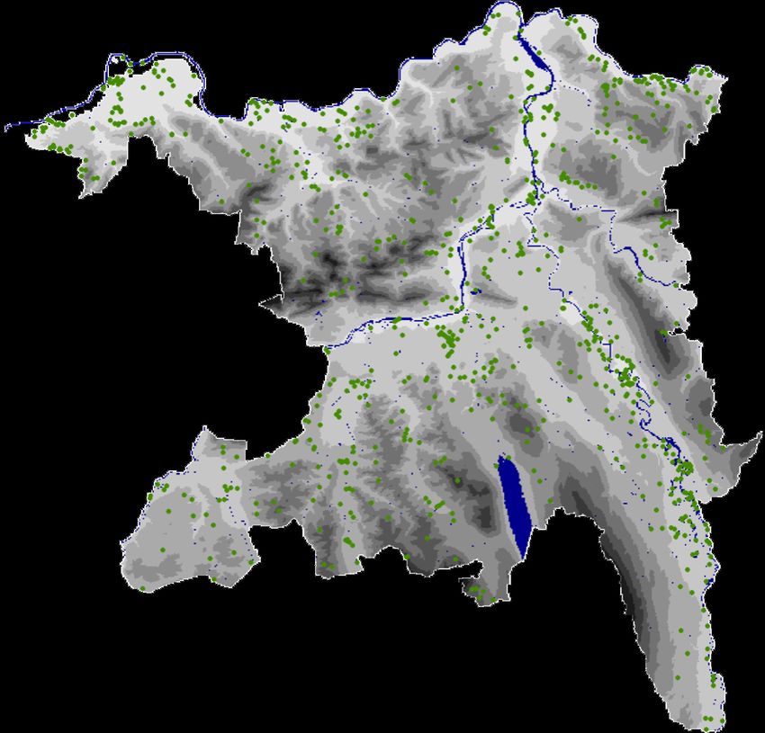
Abstract

Biodiversity is essential to sustain various ecosystem services. The growing human popula-
tion and associated land-use change through urbanization and intensification of agriculture
result in degradation, loss, and isolation of habitats. Largely due to this land-use change,
40 % of amphibian species are considered to decline worldwide. The concept of Blue-Green
Infrastructure (BGI) aims to alleviate conflicts between human and natural ecosystems. In
this study, occurrences of 10 amphibian species with differing habitat requirements in the
Canton of Aargau were modelled. With the aid of these species distribution models, the in-
fluence of five future land-use scenarios, which differed regarding human population growth
and the degree of governmental interventions, was assessed. Two existing landscape in-
ventories supporting biodiversity were regarded as starting points to identify regions with
existing and missing BGI coverage. My findings revealed that scenarios with a higher de-
gree of urbanization resulted in a higher change of modelled biodiversity hotspot areas,
which resulted not only in losses but also in gains. The results suggest that gains on future
urban areas can occur provided that the surrounding coverage within a focal window of
300 x 300 m remains on average below 70 % regarding urban land use and above 20 %
concerning forest coverage. As urbanization in the included land-use scenarios is mostly
predicted in flat areas near the main rivers of the Canton encompassing primary habitats for
many amphibian species, biodiversity hotspot losses were mostly predicted in these areas.
Therefore, a continuation of the displacement of amphibians into secondary habitats was
predicted. As habitat requirements vary severely between amphibian species, BGI needs to
be planned and managed as diversely as possible. For instance, the comparison of the two
species with the most extreme predicted future changes suggested that Epidalea calamita
might establish in urban areas, while Salamandra salamandra probably profits more from
consistent protection of forests. This underlines the importance of deriving BGI in both
urban and rural environments. 18 % of the modelled amphibian biodiversity hotspot ar-
eas in the study area resulted to be covered by existing landscape inventories with legally
binding protection goals and can be regarded as already having a network of BGI. However,
other regions like the Southwest of the Canton of Aargau, where additionally several models
agreed on predicting biodiversity loss, were found to lack coverage. To sustain biodiversity
and associated ecosystem services in the long-term, this finding could support decisions
for additional legally binding conservation strategies in these areas.

Keywords: Amphibians, Biodiversity, Blue-Green Infrastructure, Human-dominated Land-
scapes, Land-use change, Scenarios, Species distribution models

                                                                                           iii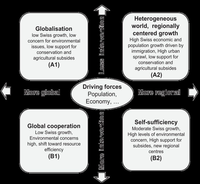
Table of Contents

Abstract                                                                                                                                                                  iii

1 Introduction                                                                                                                                                             1

2 Material and Methods                                                                                                                                                     3
  2.1 Study Area . . . . . . . . . . . . . . . . .       .   .   .   .   .   .   .   .   .   .   .   .   .   .   .   .   .   .   .   .   .   .   .   .   .   .   .   .     3
  2.2 Landscape Inventories . . . . . . . . . .          .   .   .   .   .   .   .   .   .   .   .   .   .   .   .   .   .   .   .   .   .   .   .   .   .   .   .   .     3
  2.3 Study Species . . . . . . . . . . . . . . .        .   .   .   .   .   .   .   .   .   .   .   .   .   .   .   .   .   .   .   .   .   .   .   .   .   .   .   .     4
  2.4 Environmental Predictors . . . . . . . .           .   .   .   .   .   .   .   .   .   .   .   .   .   .   .   .   .   .   .   .   .   .   .   .   .   .   .   .     4
      2.4.1 Future land-use scenarios . . .              .   .   .   .   .   .   .   .   .   .   .   .   .   .   .   .   .   .   .   .   .   .   .   .   .   .   .   .     7
  2.5 Species Distribution Modelling (SDM)               .   .   .   .   .   .   .   .   .   .   .   .   .   .   .   .   .   .   .   .   .   .   .   .   .   .   .   .     8

3 Results                                                                                                                                                                 12
  3.1 Model Assessment . . . . . . . . . . . . . . . . . . . . . . . . . . . . . . . . . . . . . . . .                                                                    12
  3.2 Effects of future land-use scenarios on amphibian biodiversity hotpots . . . . . .                                                                                  12
      3.2.1 Land-use predictor change on areas of biodiversity hotspot changes . . .                                                                                      14
      3.2.2 Amphibian biodiversity hotspot change on future urban areas . . . . . . .                                                                                     14
  3.3 Effects of future land-use scenarios on individual species . . . . . . . . . . . . . . .                                                                            15
      3.3.1 Composition of the species on modelled biodiversity hotspots . . . . . . .                                                                                    15
      3.3.2 Effect of future land change on individual species . . . . . . . . . . . . . . .                                                                              16
  3.4 Landscape inventories as a starting point for BGI to support amphibian biodi-
      versity hotspots . . . . . . . . . . . . . . . . . . . . . . . . . . . . . . . . . . . . . . . . . .                                                                17

4 Discussion                                                                                                                                                              19
  4.1 Model Assessment . . . . . . . . . . . . . . . . . . . . . . . . . . . . . . . . . . .                                                         . . . . .            19
  4.2 Effects of future land-use scenarios on amphibian biodiversity hotspots                                                                        . . . . .            19
  4.3 Effects of future land-use scenarios on individual species . . . . . . . . . .                                                                 . . . . .            20
  4.4 Landscape inventories as a starting point for BGI to support amphibian                                                                         biodi-
      versity hotspots . . . . . . . . . . . . . . . . . . . . . . . . . . . . . . . . . . . . .                                                     . . . . .            21
  4.5 Limitations . . . . . . . . . . . . . . . . . . . . . . . . . . . . . . . . . . . . . . . .                                                    . . . . .            21

5 Conclusion                                                                                                23
  5.1 Outlook . . . . . . . . . . . . . . . . . . . . . . . . . . . . . . . . . . . . . . . . . . . . . . . 23

Acknowledgements                                                                                                                                                          25

Literature                                                                                                                                                                26

A Appendix                                                                                                                                                                   I
  A.1 Methods . . . . . . . . . . . . . . . . . . . . . . . . . . . . . . . . . . . . . . . . . . . . . . .                                                                  I
      A.1.1 Species data . . . . . . . . . . . . . . . . . . . . . . . . . . . . . . . . . . . . . . . .                                                                     I
      A.1.2 Predictor rasters . . . . . . . . . . . . . . . . . . . . . . . . . . . . . . . . . . . . .                                                                    III
      A.1.3 Correlation and variance inflation of the predictors . . . . . . . . . . . . . . .                                                                            IV
      A.1.4 Spatial representation of the land-use changes in the future scenarios . .                                                                                      V
  A.2 Results . . . . . . . . . . . . . . . . . . . . . . . . . . . . . . . . . . . . . . . . . . . . . . . .                                                             VII
      A.2.1 Model evaluation . . . . . . . . . . . . . . . . . . . . . . . . . . . . . . . . . . . . .                                                                    VII
      A.2.2 Dynamic predictors of changing biodiversity hotspot areas on future ur-
            ban areas . . . . . . . . . . . . . . . . . . . . . . . . . . . . . . . . . . . . . . . . . .                                                                VIII
      A.2.3 Effect of future land-use scenarios on individual species . . . . . . . . . . .                                                                               IX

Declaration of Originality                                                                                                                                               XIII

                                                                                                                                                                           iv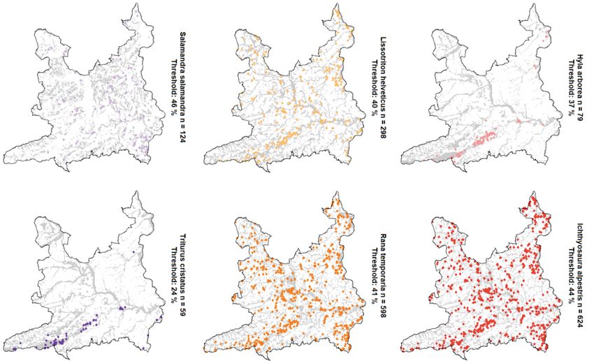
Lucie Roth, 31 March 2021

1. Introduction
Biodiversity is defined as the variety and diversity of life on the levels of genes, species, and
ecosystems (Carreon-Lagoc et al. 1994). It is of fundamental importance to support diverse
ecosystem services, as the efficiency of ecological communities to capture, produce and
recycle nutrients increases with biodiversity (Cardinale et al. 2012). Ecosystem services
include a wide range of processes from the purification of air and water, increasing soil fer-
tility, mitigation of floods and droughts to the provision of recreational areas (Daily 2003).
These services are globally essential for human civilization and well-being in both urban
and rural environments (Bolund and Hunhammar (1999), Kroll et al. (2012)). Additionally,
biodiversity increases the resilience of ecosystems, which may be an important foundation
to ensure that future generations can continuously profit from ecosystem services under
projected human-induced changes (Oliver et al. 2015).

However, intensification and expansion of human land use in the past decades have heav-
ily influenced biodiversity (Foley et al. 2005) on all levels regarding genetic, species, and
ecosystem diversity (Hansen, DeFries, and Turner 2004). The ongoing growth of the world’s
human population results in increasing land-use demand of both urban and agricultural ar-
eas (Döös 2002). Land-use change often occurred at the expense of areas like wetlands and
forests, which provide important ecosystem services and are rich in biodiversity (Lindquist
et al. (2012), Sica et al. (2016)). Concerning wetlands, an estimated 50 % were lost globally
due to the conversion to urban and agricultural areas (Rijsberman and Silva (2006), Gard-
ner, Barchiesi, et al. (2015)). Urbanization is usually linked with loss and fragmentation of
habitats, alteration of water and nutrient cycles, and changes in the composition of species
(Crooks and Soulé (1999), O’Driscoll et al. (2010), Lin et al. (2014), Liu, He, and Wu (2016)).
Agricultural intensification often leads to high levels of nutrients, pesticides, monocultures,
and intensive grazing or cutting of grasslands, which are all unfavourable to sustain a high
level of biodiversity (Plantureux, Peeters, and McCracken (2005), Karp et al. (2012), Brühl
et al. (2013), Tsiafouli et al. (2015), Raven and Wagner (2021)).
Amphibians are highly threatened through land-use change and associated habitat loss and
fragmentation (Cushman (2006), Becker et al. (2007)). Among vertebrates, amphibians are
the most threatened group in the world and over 40 % of the known species are considered
in decline (Stuart et al. (2004), IUCN (2020)). Around 90 % of the threatened amphib-
ians are impacted by urbanization (Baillie, Hilton-Taylor, and Stuart 2004). Depending on
the season and stage of life, amphibians need both aquatic and terrestrial habitats. This
requirement is in conflict with the decline of suitable semiaquatic habitats like wetlands.
Amphibians have a key role regarding nutrient flow and recycling of both aquatic and terres-
trial ecosystems, as they are predators and prey at the same time (Crump 2009). However,
there are important differences between habitat preferences of amphibian species, for in-
stance the degree of specialization. While some amphibian species like Rana temporaria
are classified as generalists as they have few habitat requirements (Flory 1999), specialists
like Salamandra salamandra are found in a narrower subset of ecological conditions (Küry
2003). Additionally, pioneering species like Epidalea calamita colonize dynamic habitats in
an early successional state (Snep and Ottburg 2008). For the design of conservation strate-
gies, species-specific requirements should be taken into account (Cushman (2006), Brown
et al. (2012), Klaus and Noss (2016)).

The conceptual framework of Blue-Green Infrastructure (BGI) aims to balance conflicts be-
tween natural and human ecosystems (Benedict, McMahon, et al. (2002), Kowarik, Fischer,
and Kendal (2020)). According to the European Commission (2013), BGI is defined as a
strategically planned network of natural and semi-natural blue (aquatic) and green (terres-
trial) areas. They are designed and managed to deliver a wide range of ecosystem services
both in urban and rural settings. In urban areas, BGI might help to restore ecosystem ser-
vices like microclimate regulation to reduce the urban heat island effect (Gunawardena,
Wells, and Kershaw 2017), improve the air quality (Hewitt, Ashworth, and MacKenzie 2020)
as well as human well-being (Völker and Kistemann 2013), and provide habitats for a sur-

ETH Zürich - Master’s thesis                                                                   1

Lucie Roth, 31 March 2021

prisingly high diversity of species (McKinney 2008). Through strategical management of
forests and agriculture, BGI can be combined with existing protected areas or landscape
inventories, to enhance structural connectivity across the landscape and improve the pro-
vision of ecosystem services like pollination and carbon retention (Hermoso et al. 2020).
Maes et al. (2015) underlines that substantial investments in the development of BGI are
needed to offset land losses resulting from increasing human population, whereof both
ecosystems and society might benefit. Due to their need for semiaquatic habitats, amphib-
ians are one of the vertebrate groups that can profit from the establishment of BGI (Hamer
and McDonnell (2008), Holzer (2014)). This is why I investigated how amphibian distribu-
tions might be affected by future land-use changes to identify regions with an increased
need for BGI. Five future land-use scenarios developed by Price et al. (2015) for Switzerland
were included for this purpose. These scenarios are based on forecasts of socio-economic
developments expected until the year 2035. One of the aims of Price et al. (2015) was to
identify regions with a high risk of urbanization, which provides a promising opportunity to
investigate the influence on future biodiversity. The Canton of Aargau, located in the Swiss
Central Plateau, was taken as a case study as it belongs to the most populated and frag-
mented regions of Switzerland (Jaeger, Bertiller, and Schwick 2007), but has at the same
time a high responsibility for the national conservation of amphibians. Mainly the low, cli-
matically mild locations along the rivers Aare, Reuss, Limmat, and Rhine are part of the
distribution area of endangered species (Flöss 2009). Flory (1999) describes that primary
habitats along the rivers were lost due to human land-use change to a large extent, which
resulted in the displacement of species to secondary habitats.

Possible future distributions of 10 amphibian species differing in habitat preferences in the
Canton of Aargau were modelled. Species distribution models (SDMs) allowed investigating
the influence of five future land-use scenarios. This aimed to identify suitable starting points
for the development of BGI to support the diversity of amphibian species by addressing the
following research questions:
  1. How do different land-use scenarios influence amphibian biodiversity hotspot areas in
     the Canton of Aargau? Which land-use categories are the most important drivers of
     the change? Based on the findings of Becker et al. (2007) and Hamer and McDonnell
     (2008), I expect scenarios with higher growth in economy and population (leading to
     more urban sprawl) and less support for environmental concerns (leading to more in-
     tensive agriculture and abandonment of pasture agriculture) to show higher losses in
     biodiversity. Urbanization was reported as a decisive driver of amphibian decline (Bail-
     lie, Hilton-Taylor, and Stuart (2004), Scheffers and Paszkowski (2012)). Therefore, I laid
     a special focus on urbanizing areas with the question How does modelled biodiversity
     change on future urban areas?
  2. Hamer and McDonnell (2008) see the utility in combining both species-specific and
     community diversity approaches for amphibian conservation. This is addressed in the
     following questions: Which species occur in current biodiversity hotspots and what
     are likely changes in the future given changing land use? Which species show most
     extreme changes given future land-use scenarios and why?
  3. If existing landscape inventories are considered as starting point for a network of
     blue-green infrastructure (BGI): where are modelled amphibian biodiversity hotspots
     already covered and which regions require additional protection? This question is
     based on the work of Hermoso et al. (2020), who designed a network of BGI across the
     European Union with protected areas as a starting point.
Deepening the understanding of how different land-use scenarios influence amphibian bio-
diversity, as well as individual species, could contribute to plan and implement BGI that
supports amphibian conservation. This ultimately aims at supporting biodiversity and en-
suring attached ecosystem services for future generations, which is in accordance with the
Federal Council’s Swiss Biodiversity Strategy (BAFU 2017a).

ETH Zürich - Master’s thesis                                                                  2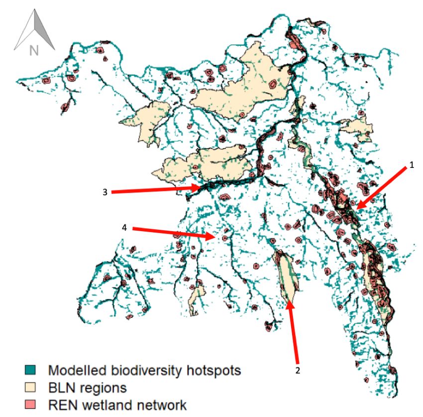
Lucie Roth, 31 March 2021

2. Material and Methods
2.1. Study Area
The study area consisted of the Canton of Aargau (1’404 km2 ) located in the North of the
Central Plateau in Switzerland. With elevations ranging from 261 to 903 m a.s.l., Aargau
belongs to the least mountainous regions of Switzerland. Important national traffic routes
and densely populated areas fragment the landscapes (Jaeger, Bertiller, and Schwick 2007).
According to the areal statistics of 2004/09 computed by the Swiss Federal Statistical Office
(SFSO 2013), the dominant land uses and land covers include agricultural land (44 %),
forests (36 %) and settlement areas (17 %, see Figure 1a).

2.2. Landscape Inventories
There are several landscape inventories for the Canton of Aargau which are designed to
preserve ecosystem services. To identify regions with existing or missing BGI, I used two
landscape inventories. First, the Federal Inventory of Landscapes and Natural Monuments
(Bundesinventar der Landschaften und Naturdenkmäler (BLN)) aims to preserve the most
typical and valuable landscapes of Switzerland (BAFU 2017d). Among other functions, BLNs
allow formulating legally binding strategies to protect biodiversity. For each BLN of the Can-
ton, goals to preserve local fauna and habitats are formulated. 9 of the 12 BLNs encompass
amphibian breeding sites of national importance (ALG n.d.). Second, I included the national
ecological network (Réseau écologique national (REN)). It represents a vision of connected
habitats on a national scale with no legal bindings (Berthoud, Lebeau, and Righetti 2004).
The total network consists of five parts that cover different types of habitats and their
associated species. Amphibians were included as indicator species for the "wetland" part.

                               a)                                           b)
Figure 1: a) Land use and land cover of the study region (Canton of Aargau, 100 m
resolution, areal statistics of 2004/09, SFSO). b) Occurrences of 10 selected study species
were sampled at 660 locations of the Amphibian Monitoring Program of Canton Aargau.
Source of the elevation map in the background: swisstopo 2001.

ETH Zürich - Master’s thesis                                                                3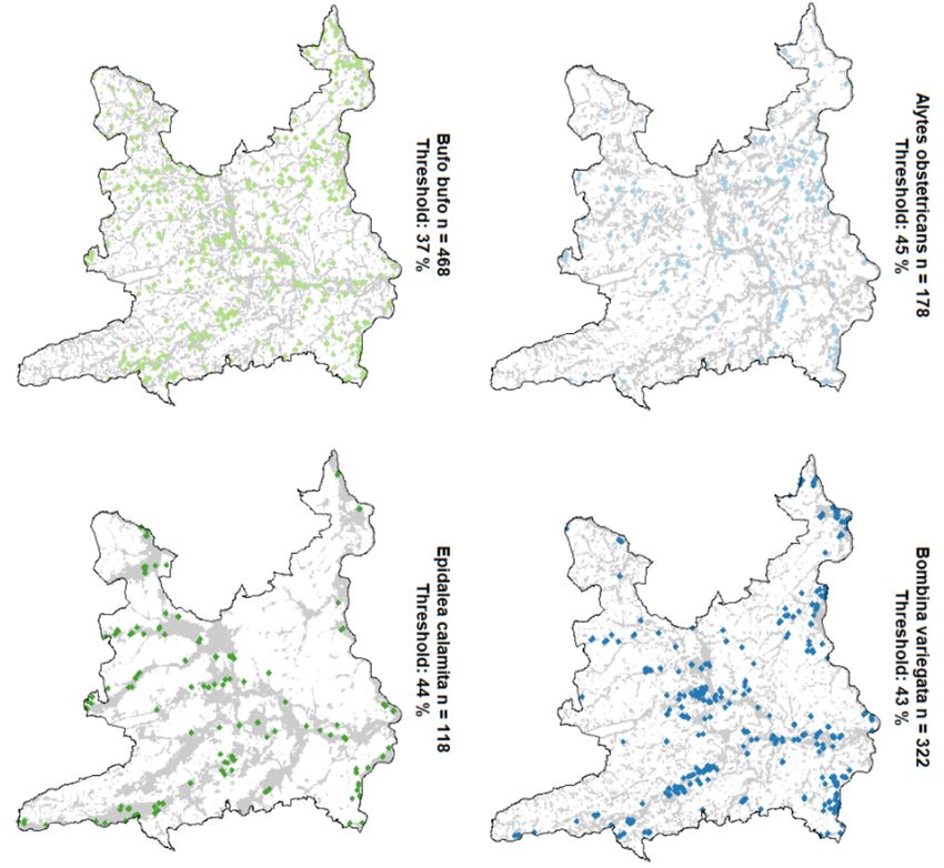
Lucie Roth, 31 March 2021

2.3. Study Species
Ten amphibian species with differing characteristics and habitat requirements were selected
as study species (Table 1). The dispersal ability and the ecological type are important char-
acteristics that determine the species ability to colonize new habitats. The maximum mi-
gration distance was regarded as a proxy for dispersal ability based on the work of Dawideit
et al. (2009). A species was regarded as present at a site if it was detected at least once
in the years between 2004 and 2013. This period was chosen to match the land-use data
(section 2.4) while providing a sufficient amount of observations for all focal species. In to-
tal, the data of 660 sampling sites (Figure 1b) of the volunteer-based Amphibian Monitoring
Program of Canton Aargau were included. Since 1999, around 300 from a total of 1’500
breeding sites are monitored every year. Each selected breeding site is visited three times
during the breeding season between April and June. Two visits occur at night and one at
daytime (Hintermann & Weber AG 2019). The individual distributions of the sampling sites
for each species can be found in Figure A.2.
Species richness is a component of biodiversity (Carreon-Lagoc et al. 1994) and was hence
used as an indicator of biodiversity hotspots. Biodiversity hotspot areas were defined as
areas where more than seven out of the ten species occur. This should ensure that at least
two of the five endangered species occur, even if all five less threatened species ("least
concern" or "vulnerable") occurred at the same site.

2.4. Environmental Predictors
The species presences were correlated to seven environmental factors (resolution of 100 x
100 m) that are relevant for the ecology of amphibians (Table 2 and Figure A.3). Four land-
use predictors (Urban and settlement areas, pasture agriculture, intensive agriculture, and
forests) originated from the areal statistics 2004/09 computed by the SFSO. The Swiss land
use and land cover statistics were interpreted from aerial photographs with a periodicity
of 12 years (SFSO 2013). The aerial photographs of Aargau for the statistic of 2004/09
were generated in 2006 and 2007 (SFSO 2004). Price et al. (2015) used six land use and
land cover categories to project future land change for the whole of Switzerland that were
considered to be affected by key land-use change processes in Switzerland: Closed forest,
Open forest, Overgrown areas, Pasture agriculture, Intensive Agriculture, and Settlement
and Urban areas. Unproductive areas like lakes and rivers were assigned as NoData (NA),
as no changes are expected. Low frequencies of a category result in a high sampling error
(SFSO n.d.). This is why I combined two categories with the most similar one: "Overgrown"
with "Pasture agriculture" and "Open forest" with "Closed forest".
While the areal statistics of the SFSO of 2004/09 served to model the reference model, five
future land-use scenarios (section 2.4.1) derived by Price et al. (2015) were used to com-
pute future projections of species occurrences. I refer to the four land-use predictors as
"dynamic" predictors. In order to include the dynamic predictors in the modelling process,
the percentage of each land use within a moving window of 300 x 300 m was calculated for
each pixel with the focal function of the raster package in R (Hijmans 2020). This window
size was chosen in order to include the influence of the surrounding landscape, as amphib-
ians migrate between different types of habitats. According to Semlitsch and Bodie (2003),
the core terrestrial habitats that amphibians need for feeding and hibernation ranged within
160 to 290 m around aquatic sites.
Three predictors remained stable for the reference and the future scenarios: distance to
water, the standard deviation of elevation, and the humidity of the soil. The predictors
were tested for correlation and variance inflation (section A.1.3). Common climatic vari-
ables in SDMs, such as temperature (or elevation) and precipitation, were not included
in these models because of the very restricted area with a homogeneous climate and no
strong elevational gradients. Secondly, land use is argumented to be the more important
small-scale driver of species distributions (Luoto, Virkkala, and Heikkinen 2006) and the
highest available resolution for area-wide climate data of Switzerland is 1 km, which is 10
times higher than the resolution of the other environmental variables.

ETH Zürich - Master’s thesis                                                                 4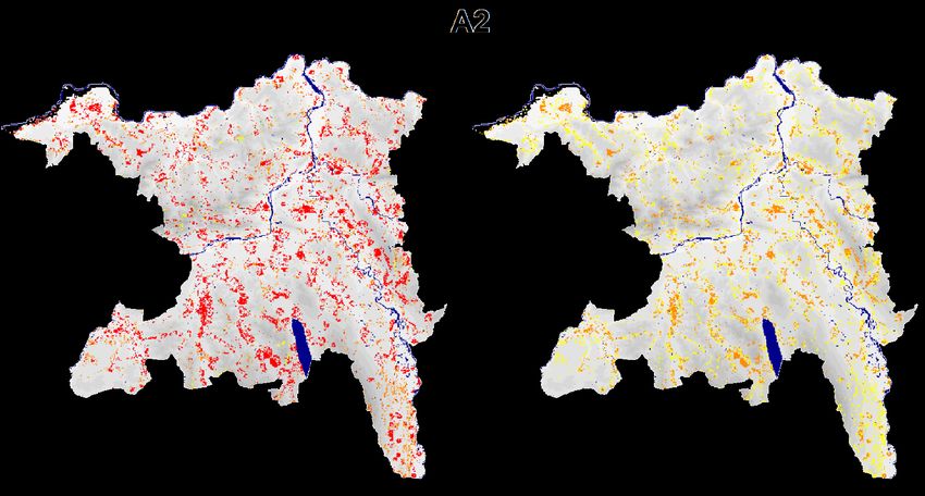
Lucie Roth, 31 March 2021
Table 1: Description of the 10 study species. The status of threats correspond to the ab-
breviations of the IUCN (2020): least concern (LC), vulnerable (VU) and endangered (EN).
Based on Dawideit et al. (2009), the maximum migration distance was regarded as an indi-
cator of dispersal distances.
(Sources: 1 Schmidt and Zumbach 2005, 2 Trochet et al. 2014, 3 Flory 1999, 4 Mermod, Zum-
bach, Borgula, Lüscher, et al. 2010, 5 Mermod, Zumbach, Borgula, Krummenacher, et al.
2010, 6 Mermod, Zumbach, Aebischer, et al. 2010, 7 Mermod, Zumbach, Lippuner, et al.
2010, 8 Grossenbacher 2014, 9 Küry 2003, 10 Scheuber 2014)
Number of Maximum
Status
sampling migration Ecological
Taxon Family of Distribution in the Canton of Aargau
locations distance Type3
Threat1
2004 - 2009 [m] 2
In the Canton of Aargau, the species is found in
hilly areas, but diminished on its original habitat
on sunny areas of floodplains. Gravel pits and
Alytes
Alytidae EN 178 500 Specialist agricultural areas on slopes are important
obstetricans
secondary habitats3. Suited terrestrial habitats
have to be found in the immediate vicinity of
spawning grounds4.
The species is found in floodplains and adjacent
slopes. Gravel pits are important secondary
Bombina Specialist, habitats, while hill areas are avoided3. The
Bombinatoridae EN 322 3'800
variegata Pioneer species is specialized on dynamic habitats and
colonizes temporary, small water bodies that
have little vegetation5.
Particularly common on wooded slopes of river
valleys if larger standing and persistent water
bodies are present. If no wooded slopes are
Bufo bufo Bufonidae VU 468 4'000 Generalist found in the vicinity of the spawning waters,
long migration distances are possible. This can
lead to conflicts on some street crossing
points3.
The toads use exclusively short-lived,
temporary water bodies for reproduction.
Therefore, it is not uncommon that the location
is changed annually. The species is now only
Epidalea Specialist, found in secondary habitats. Large construction
Bufonidae EN 118 2'600
calamita Pioneer sites are ideal habitats in the short term.
Original ideal habitats would be found along of
dynamic rivers3. Due to the usually static nature
of garden ponds, they provide no suitable
habitat for the species6.
Typical inhabitant of natural river landscapes.
All inventoried habitats are secondary habitats.
Specialist, Vital, but strongly isolated populations are for
Hyla arborea Hylidae EN 79 12'570
Pioneer instance found in the Reuss valley3. In general,
suitable habitats are not located in the vicinity
of urban areas7.
Very abundant and widespread species. It
Ichthyosaura
Salamandridae LC 624 1'000 Generalist prefers stagnant waters3. Of all species, it can
alpestris
probably profit most from garden biotopes8.
Lissotriton Very widespread species which prefers mild
Salamandridae VU 298 400 Generalist
helveticus and sunny habitats3.
The species is very abundant and can be found
Rana nearly in the whole canton. Especially common
Ranidae LC 598 2'214 Generalist
temporaria along rivers and creeks. It is the species with
fewest habitat requirements3.
The forest is the typical habitat of the species9.
Salamandra Ideal spawning grounds are pristine and clean
Salamandridae VU 124 30 Specialist
salamandra streams with no fish. Not found in urban and
intensive agricultural areas3.
The species occurs along streams and in bogs. It
is very seldom in the Canton. It used to occur in
Triturus flood plains. Streets and settlements isolate
Salamandridae EN 59 1'290 Specialist
cristatus populations3. Ideal spawning grounds are about
half a meter deep, rich in submerged
vegetation and partially sunny10.
ETH Zürich - Master’s thesis 5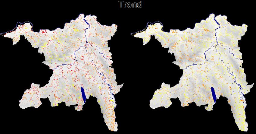
ETH Zürich - Master’s thesis
Table 2: Seven environmental predictors were used to model the occurrence of the 10 study species.
Expected response of
Type Predictor Unit Ecological importance Geodata source Processing steps
distribution
Urbanization changes the hydrology, Decrease with higher values
Urban/settlement areas modifies soils and can cause habitat (Hamer and McDonnell
fragmentation and loss (McKinney, 2006). 2008)
Depending on the species:
there are forest specialists, The land-use categories of the SFSO were
Forests influence the light availability,
but some species Areal statistics aggregated by Price et al. (2015). For this thesis,
Forest temperature and hydrology of a habitat
Dynamic predictors
Coverage in % prefer more open and 2004/09 made by the categories "Open Forest" and "Closed
(Schäfer and Dirk 2011).
within a focal sunny habitats the SFSO. In the Forest" were combined. The category
window of (Halverson et al. 2003). canton of Aargau, "Overgrown" was added to "Pasture
300 x 300 m the aerial pictures agriculture". For each land use, the focal
around each Wet soils were often drained to create were taken in percentage within a moving window of
pixel. suitable agricultural land. This destructed 2007 and 2008 9 neighbouring pixels was
Intensive agriculture Increase for species that
amphibian primary habitats. However, (SFSO 2004). calculated with the aid of the focal function of
prefer open and sunny
agricultural ponds can serve as important the raster package in R (Hijmans 2020).
habitats. An important
secondary habitats for amphibians
prerequisite are suitable
(Knutson et al. 2004) that prefer open and
water bodies or wet soils
Pasture agriculture sunny habitats. High levels of nutrients and
(Halverson et al. 2003).
pesticides can harm amphibians
(Brühl et al. 2013).
Amphibian larvae develop in water. The Calculation of the euclidean distance to reed
dependency of adults depends on the belts, stagnant and flowing water bodies (raster
Cantonal
Distance to water m species: some species are only at the water Increase with lower values resolution 2 x 2 m) with the distance function of
cadastral map
for mating while others spend the whole the raster package (Hijmans 2020). Aggregation
year in ponds (karch n.d.). to 100 x 100 m.
Stable Predictors
Descombes et al.
Continuous (2020) modelled
gradient the soil moisture.
Humidity is needed to prevent the moist
Lucie Roth, 31 March 2021
between Increase with increasing It is based on the
Soil moisture (EIV_F) skin of amphibians from drying out −
1 (dry soil) to values ecological
(karch n.d.).
5 (plants growing indicator values
in water) (EIV) from Landolt
et al. (2010).
Steeper soils can pose an obstacle for Calculation of the standard deviation of
Standard deviation of
m amphibian movement and drain quicker Increase with lower values swisstopo (2001) elevation within 100 x 100 m of pixels in
elevation
(Lowe et al. 2006, Ribeiro et al. 2018). the size of 25 x 25 m.
McKinney (2006), Schäfer and Dirk (2011), Knutson et al. (2004), Brühl et al. (2013), Karch (n.d.), Lowe et al. (2006), Ribeiro Jr. et al. (2018), Hamer and McDonnell (2008), Halverson et al. (2003), SFSO (2004), Descombes et al. (2020), swisstopo (2001), Hijmans (2020)
6Lucie Roth, 31 March 2021 2.4.1. Future land-use scenarios Price et al. (2015) developed five different land-use change scenarios which are based on the same categories as the reference land use (areal statistics of the SFSO for 2004/09). The study was conducted to identify likely risk areas of urbanization and land abandonment in Switzerland. The Trend scenario is the linear projection to 2035 of observed land-use trends between the areal statistics from 1985, 1997, and 2009. Although no explicit time step was chosen for the modelling of the other four scenarios, 2035 served as a time horizon relevant to policy and planning and matching cantonal level growth scenarios. The four scenarios were modelled using the Dyna-CLUE land-use modelling framework (Verburg and Overmars 2009) by incorporating socio-economic and bio-geographical variables. The two main axes of driving forces were regional vs. global development and more vs. less intervention. This resulted in different proportions of the land-use categories (Figure 2). As described in Price et al. (2015), the "A" scenarios are considered as the market-driven scenarios, while the "B" scenarios are driven by high interventions. The urban and settlement areas increase in all scenarios due to population growth scenarios developed by the SFSO (2010). The highest increases in urban areas are predicted for scenario A2, followed by the scenarios Trend and B2. In line with general trends predicted for Europe (Rounsevell et al. 2005), agricultural land is expected to decrease between 9 (scenario B1) and 25 % (A2) by 2040, with lower losses of pasture agriculture than of the category of intensive agriculture. Concerning the forest areas, it was expected that the current restrictions that allow no net loss (FOEN 2013) would remain in the future. A1 shows high levels of agricultural land abandonment, which results in the highest increase of the Overgrown land-use category. Scenario A2 has the most extreme changes in land-use patterns. B1 has nearly no changes. A slight increase in the agricultural area is foreseen for the self-sufficiency scenario B2. A spatial representation of the areas that changed in land use is shown in Figure A.6 for each scenario. Across all scenarios, urbanization is mainly occurring at the expense of agricultural areas. The changes in the Trend scenario are spatially more scattered than in the other scenarios. ETH Zürich - Master’s thesis 7
Lucie Roth, 31 March 2021

                                                               A1              [km2]                            A2              [km2]
                                                               Closed forest    511                             Closed forest    512
                                                               Open forest       2.4                            Open forest       0.3
                                                               Overgrown         23                             Overgrown         13
                                                               Pasture                                          Pasture
                                                                                160                                              104
                                                               agriculture                                      agriculture
                                                               Intensive                                        Intensive
                                                                                424                                              386
                                                               agriculture             Reference: 2004/09       agriculture
                                                               Urban/                  Closed forest      509   Urban/
                                                                                247                                              352
                                                               settlement                                       settlement
                                                                                       Open forest        1.1
                                                                                       Overgrown          0.4
                                                                                       Pasture
                                                                                                          206
                                                                                       agriculture
                                                               B1              [km2]
                                                                                       Intensive                B2              [km2]
                                                               Closed forest     511                      412
                                                                                       agriculture              Closed forest     510
                                                               Open forest       0.4   Urban/
                                                                                                          238   Open forest       0.3
                                                               Overgrown         0.3   settlement
                                                                                                                Overgrown          0
                                                               Pasture
                                                                                 170                            Pasture
                                                               agriculture                                                        158
                                                                                                                agriculture
                                                               Intensive
                                                                                 443                            Intensive
                                                               agriculture                                                        426
                                                                                                                agriculture
                     a)                                        Urban/
                                                               settlement
                                                                                 242                 b)         Urban/
                                                                                                                                  272
                                                                                                                settlement

                                    Trend              [km2]
                                    Closed forest       511
                                    Open forest          0.4
                                    Overgrown            10
                                    Pasture
                                                        148
                                    agriculture
                                    Intensive
                                                        427
                                    agriculture
                                    Urban/
                                                        272
                                    settlement

                                                  c)
Figure 2: Five land-use scenarios developed by Price et al. (2015) were used to project
future species distributions. a) Four were modelled according to two axes (Figure extracted
with permission by Price et al. (2015)), which resulted in different proportions of the land
uses b). The fifth scenario is a linear extrapolation of the changes observed between the
SFSO areal statistics of 1985, 1997, and 2009 (Trend scenario, c)).

2.5. Species Distribution Modelling (SDM)
The species occurrence data and the environmental predictors were combined to model
presence-only SDMs using the BIOMOD2 platform (Thuiller, Georges, et al. (2020), Version
3.4.6) in R (R Core Team (2019a), Version 3.6.1). An overview of the modelling process can
be found in Figure 3.

  1. Reference model input: For each species, four sets of randomly selected pseudo-
     absences were used for modelling. Barbet-Massin et al. (2012) showed that random
     distribution of the pseudo-absences yielded the most reliable predictions of species
     distribution for most model types. The pseudo-absence number was set to be three
     times higher than the presence frequency (Table 1). This is in line with the recommen-
     dation of Liu, Newell, and White (2019) to favor a small over a large multiplication fac-
     tor between the numbers of presences and randomly distributed absence points. Ac-
     cording to Barbet-Massin et al. (2012), the ideal ratio of presences to pseudo-absences
     differs between models. This is however not applicable for the generation of ensem-
     ble models (see step 4), as they rely on evaluating predictive power compared to the
     same data for each model type.
     Both presences and pseudo-absences were set to have a minimum distance of 100 m
     between each other to match the predictor resolution and to avoid spatial autocorre-
     lation. The predictor data was prepared as described in Table 2.

ETH Zürich - Master’s thesis                                                                                                            8
ETH Zürich - Master’s thesis
Modelling process (BIOMOD2) Output analysis
Modelling
Species performance and Comparison with
occurrence data response curves existing landscape Analysis of gain and
(section 2.3) inventories loss areas on
Modelling of 3 urbanizing areas
80 models per
1
the reference
species
scenario Biodiversity
2
Environmental hotspot maps
Predictors 4 5
(section 2.4)
Future 1 Binary map
projections with Species range Predictor change
per species and
dynamic land-use change (SRC) analysis of areas
scenario
predictors per species and with gains and
(reference and
scenario losses
future)
Land use
Stable
SFSO
predictors
2004/09
Future land-use
scenarios
(Price et al. 2015).
Lucie Roth, 31 March 2021
Description
Input Output Process label
Figure 3: Overview of the modelling process (created on diagrams.net)
9Lucie Roth, 31 March 2021
2. Model set-up: In this study, five models were applied: artificial neural networks
(ANN, Ripley (1996)), flexible discriminant analysis (FDA, Hastie, Tibshirani, and Buja
(1994)), generalized boosted models (GBM, also known as boosted regression trees,
Ridgeway (1999)), generalized linear model (GLM, McCullagh (1989)) and random for-
est for classification and regression (RF, Breiman (2001)). For each focal species, 80
models were computed using the reference model predictors (5 model types x 4 sets
of pseudo-absences (see step 1) x 4 evaluation runs (see step 3)). These models were
rerun with the input data derived from the future land-use scenarios.
3. Model evaluation: As an alternative to evaluating a model on an independent data-
set, Thuiller, Lafourcade, et al. (2009) propose data-splitting procedures. A user-
defined proportion of the original data is randomly assigned as training data, while
the other part is used to validate the model. To decrease the effect of the random
assignment, the procedure can be repeated several times. For this study, 70 % of
the presence data was used for training. Four repetitions of random classification into
training and testing data were applied.
The predictive power was assessed with the area under the curve (AUC) of the rela-
tive operating characteristic (ROC) curve (Hanley and McNeil 1982) and the true skill
statistic (TSS, Allouche, Tsoar, and Kadmon (2006)). AUC is independent of prevalence
as well as thresholds and considered as an effective evaluation indicator (Fielding and
Bell 1997). The values range from 0 (model systematically wrong) to 1 (perfect model),
where a value of 0.5 signifies that the model is not better than a random model. TSS
is a threshold-dependent evaluation measure that ranges from -1 to 1. 1 signifies a
perfect agreement of observations and predictors, while values below 0 indicate an
agreement no better than a random classification. As applied by Zhang et al. (2015),
subsequent ranges were used to interpret the evaluation values: AUC values < 0.7
were classified as poor, 0.7 - 0.9 as moderate and values > 0.9 as good modeling
performance (Swets 1988). TSS values below 0.4 indicated poor, 0.4 til 0.8 useful and
over 0.8 excellent models. In addition, the Boyce index was calculated which is partic-
ularly suitable for presence-only models (Hirzel et al. 2006). The values range from -1
to 1, where 1 indicates consistency between the predicted and observed presences.
4. Ensemble modelling and binarization: As described above, three sources intro-
duce substantial randomness to the process of modelling: the random selection of
pseudo-absences, the arbitrary assignment of the presences records into training and
evaluation data as well as intermodel variance. To account for these variabilities,
BIOMOD2 offers the possibility to form ensemble forecasts, where a range of different
models generated by different methods and conditions is combined (Araújo and New
2007). Several options for this combination are available. For this study, the weighted
mean method was chosen. In contrary to unweighted methods like committee averag-
ing, weights are assigned depending on the predictive performance of the individual
models. According to Marmion et al. (2009), the weighted mean method results in the
most robust models and it is the most frequently used combination method (Hao et al.
2019). In this study, the weights were assigned based on the TSS and AUC values. In
a pre-selection, models with a low predictive power (TSS < 0.4 and AUC < 0.7) were
excluded.
The binarization transforms continuous probabilities of occurrences into binary values
for occurrences (presence or absence). I used the threshold that maximizes the TSS
to define the threshold of binarization. According to Liu, White, and Newell (2013), it
is a suitable method of binarization for presence-only data-sets.
5. Output analysis: In order to investigate the research topics defined in section 1, the
modelling output was analyzed as follows:
(a) To assess the influence of the different future land-use scenarios on the biodiver-
sity hotspots, the values of changing areas were compared: This included the total
area of change, as well as biodiversity hotspot gain and loss areas. Thereafter,
the average change of the land-use predictors of biodiversity hotspot areas that
ETH Zürich - Master’s thesis 10Lucie Roth, 31 March 2021
changed between the reference and the future scenarios was calculated. This
should provide insights into what land-use shifts drove the changes in biodiversity
hotspots. As urbanization is expected to be an important driver of biodiversity loss
(Scheffers and Paszkowski 2012), an additional analysis of the predictor change
on areas that are predicted to be urbanized in the future was assessed, leading to
the derivation of recommendations for the implementation of BGI.
(b) The influence of the land-use scenarios was assessed on the level of the species
composition, as well as for individual species. For each species, the percentage of
gained or lost area between the reference and future scenario was calculated. The
difference between the gain and loss values is the species range change (SRC). It
is an indicator if gains (positive values) or losses (negative values) are higher. The
ten species were combined into groups of similar SRCs. Of the species with the
most extreme changes, the changes in the predictors were calculated. Reasons
for the extreme change were investigated with the help of ecological information
of the species (Table 1) and the response curves. Response curves show how the
species occurrence probability changes with increasing values of each predictor.
(c) In order to identify regions with existing or missing BGI coverage, the modelled
amphibian biodiversity hotspots of the reference scenario were compared with the
BLN regions and the "wetland" network of the REN (section 2.2).
ETH Zürich - Master’s thesis 11Lucie Roth, 31 March 2021
3. Results
3.1. Model Assessment
For each species, ensemble models were generated and evaluated (Figure 4). They were
computed with the weighted mean method based on 80 individual models per species
(Figure A.8). The TSS values range between 0.5 and 0.8 and are classified as "useful"
models (Zhang et al. 2015). The AUC values for Triturus cristatus and Hyla arborea are
classified as "good" models, while the others rank "moderate" (Swets 1988). All Boyce
indexes rank higher than 0.9, most even above 0.99 (Figure A.7). This indicates a high
consistency between modelled and observed presences (Hirzel et al. 2006).
Figure 4: AUC versus TSS values of the ensemble models (reference scenario) that were
calculated with the weighted mean method. The grey line corresponds to the AUC-threshold
that separates “moderate” from “good” model performance (Swets 1988). The TSS values
are all in the range of “useful” models (Zhang et al. 2015)
3.2. Effects of future land-use scenarios on amphibian biodiversity
hotpots
Modelled biodiversity hotspots of the reference scenario encompassed 270 km2 . This corre-
sponds to about one fifth of the Canton of Aargau. The total changes in biodiversity hotspot
areas (Figure 5) ranged between 6 (scenario B1) and 32 km2 (scenario A2). The highest
absolute losses are observed in scenario A2 (19 km2 ), followed by Trend (12 km2 ) and sce-
nario B2 (9 km2 ). The highest absolute gains are observed in scenarios A2 (14 km2 ), Trend
(7 km2 ), and A1 (5 km2 ). Area loss was slightly higher than area gain in all scenarios. How-
ever, gains and losses contributed nearly equally to the total areas of change. At least two
models agreed on predicting losses on 12 km2 and gains on 7 km2 (Figure 5, lower right
panel).
ETH Zürich - Master’s thesis 12Lucie Roth, 31 March 2021
A1: change on 11.02 km² A2: change on 32.28 km²
Loss: 5.66 km² Loss: 18.66 km²
Gain: 5.36 km² Gain: 13.62 km²
B1: change on 6.13 km² B2: change on 13.25 km²
Loss: 3.67 km² Loss: 8.53 km²
Gain: 2.46 km² Gain: 4.72 km²
Trend: change on 19.15 km² Model agreement
Loss: 11.79 km²
Gain: 7.36 km²
Loss predicted by at least 2 models: 12.49 km²
Gain predicted by at least 2 models: 6.89 km²
Main lakes and rivers
Figure 5: Changes in modelled amphibian biodiversity hotspot areas: the total changes
(indicated in the figure titles) ranged between 6 and 32 km2 . Gain and loss areas con-
tributed nearly equally to the total areas of change. The panel on the bottom right shows
the areas where at least two models agreed on predicting gains or losses.
ETH Zürich - Master’s thesis 13Lucie Roth, 31 March 2021
3.2.1. Land-use predictor change on areas of biodiversity hotspot changes
The change of the four dynamic land-use predictors was analyzed to gain insights into
which categories drove the change in modelled biodiversity hotspots. The dynamic predic-
tors consisted of the percentage that was covered by the corresponding land-use category
within a focal window of 300 x 300 m (Table 2). Table 3 shows the average change of all
pixels with hotspot gains or losses between the reference and the future scenarios.
Modelled biodiversity hotspot loss areas showed nearly no change in the percentage of for-
est areas, while pastures decreased in all scenarios. In scenarios A1 and Trend, pastures
decreased by around - 11 %. Given A2, B1, and B2 pastures decreased by around - 16 %.
Furthermore, the change in share of intensive agricultural area showed no consistent trend
between the scenarios: while scenarios A1 and B1 showed a moderate (+ 4.7 %) or strong
(+ 13 %) increase, scenarios B2 and Trend showed a moderate (- 3.6 %) and A2 a strong
decrease (- 17 %) of intensive agriculture. The highest values of change were usually found
in the percentage of urban change. A2 showed the highest increase (+ 33 %). B2 and
Trend showed intermediate increases (+ 14 and + 19 %), while A1 and B1 showed lowest
increases (+ 4 and + 6 %, Table 3a).
Modelled biodiversity hotspot gain areas showed similar trends like the loss areas: pasture
agriculture decreased and no consistent change is shown in the change of intensive agri-
culture. Urban areas increased as well, however less than in areas with losses. While the
percentage of forest areas did nearly not change on loss areas, the values increased on all
gain areas.
Table 3:The highest
Average increases
percentage change were
in land observed inof
use predictors scenario A1hotspots
biodiversity with +between
12 % andthe in B1 with
+ 2.5 reference
% (Figure 3b).
and future scenarios. a) Loss areas and b) gain areas of modelled amphibian biodiversity
Table hotspots.
3: Average percentage change in land-use of modelled biodiversity hotspots be-
tween the reference and future scenarios on a) biodiversity hotspot loss areas and b) gain
areas.
a) b)
3.2.2. Amphibian biodiversity hotspot change on future urban areas
Urbanization is regarded as a decisive land-use change factor that decreases biodiversity
(section 1) and was therefore subject of particular interest. I focused on areas that were
predicted to become urbanized between the reference and the future scenarios and ad-
ditionally showed changes in biodiversity hotspot areas. Several differences could be ob-
served when comparing the dynamic predictors (coverage per land-use category within 300
x 300 m) of biodiversity hotspot gain and loss areas. The percentage of surrounding urban
coverage increased in all scenarios compared to the reference (Land-use (LU) 04/09). How-
ever, urban coverage was lower for biodiversity hotspot gain areas compared to loss areas.
All medians of urban percentage on gain areas remained below 70 % in the future scenarios
(Figure A.9a). All biodiversity gain areas showed a higher forest percentage (medians > 20
%) compared to loss areas (medians ∼ 0 %, Figure A.9b). The change of the two predictors
representing surrounding coverage of agricultural land use was not ambiguous. Generally,
the coverage of intensive and pasture agriculture decreased between the reference and
the future scenarios. However, the percentages of biodiversity hotspot gain and loss areas
were not significantly different from each other (Figure A.9c and d).
Modelled biodiversity hotspot loss on future urban areas mostly occurred at lower distances
to water (< 200 m), a lower standard deviation of elevation (< 3 m), and higher soil moisture
ETH Zürich - Master’s thesis 14Lucie Roth, 31 March 2021 (value ∼ 3) than biodiversity hotspot gain areas (upper panels of Figure 6). These values can be compared to the frequency distribution of all areas that are predicted to be urbanized in the future (lower panels of Figure 6). Similar values are observed for the most frequent future urban areas as well as for areas predicting biodiversity hotspot loss. Figure 6: The boxplots (upper panels) show the values of the stable predictors of future urban areas that were predicted to have biodiversity hotspot gains or losses. Gains usually occurred in areas with a higher distance to water, a higher standard deviation, and lower soil moisture than loss areas. The histograms (lower panels) show the distribution of the stable predictors on all future urban areas. Similar predictor values are observed for the predicted biodiversity hotspot loss areas as for the most frequent future urban areas. 3.3. Effects of future land-use scenarios on individual species Different habitat requirements of the species (Table 1) require adaptive conservation man- agement strategies (e.g. Cushman (2006)). Therefore, Hamer and McDonnell (2008) sug- gest including considerations on the level community diversity as well as species-specific requirements. 3.3.1. Composition of the species on modelled biodiversity hotspots From the more threatened species (classified as "EN", Table 1), Alytes obstetricans (∼ 22 km2 ) followed by Hyla arborea (∼ 20 km2 ) covered the largest modelled biodiversity hotspot areas. The five least threatened species had the largest areas (each ∼ 26 km2 ). The differences in the areas between the scenarios are low, but scenario A2 usually had the highest reductions in projected biodiversity hotspots per species compared to the reference scenario (Figure A.10). ETH Zürich - Master’s thesis 15
Lucie Roth, 31 March 2021

3.3.2. Effect of future land change on individual species
The species range change (SRC, Table 4) is calculated as the difference between the per-
centage of gained and lost area in the future scenario compared to the reference scenario
(see Figure A.1 for gain and loss values). Therefore, it indicates if gains (positive values) or
losses (negative values) are higher, or if gains and losses are about in the same order of
magnitude (neutral values).
A2 showed the most extreme changes followed by the Trend and B2 scenario. The lowest
average changes were observed for scenarios A1 and B1. Three major patterns of SRC-
responses were identified among all species: i) Epidalea calamita and Bombina variegata
both showed positive values in all scenarios. Therefore, they were classified as the "high
gain" group. ii) In contrast, Salamandra salamandra showed negative values in all scenar-
ios and was hence classified as "high loss". iii) The SRC of all other species ranged between
± 3% in the majority of the scenarios, as gains and losses were nearly the same ("neutral
group").

Table 4: Species range change (SRC, percentage of gains minus percentage of losses,
Table A.1) for each species and scenario. Three response groups were distinguished: "High
gain" (Epidalea calamita and Bombina variegata), "high loss" (Salamandra salamandra) and
"neutral" (gains and losses in the same order of magnitude, all other species).

For the further analysis, the two species with the most extreme SRC were analyzed: Ep-
idalea calamita ("high gain") and Salamandra salamandra ("high loss"). To capture the
clearest trends of possible changes, only the most extreme scenario A2 was included.
At one extreme, Epidalea calamita (representing the group of "high gains") showed almost
no increase of urban percentage in loss areas (+ 0.5 %), but a high increase of this category
in gain areas (+ 42 %, Figure A.11). This indicates that the species gained habitats in future
urban areas while no habitats were lost in urbanizing areas. On loss areas, the percentage
of intensive agriculture (+ 14 %) increased at the expense of pasture agriculture (- 16 %).
Both categories representing agricultural land use decreased on the gain areas (- 20 %).
Epidalea calamita was the only species that showed a slight increase in occurrence prob-
ability with increasing urban coverage in the focal window of 300 x 300 m (Figure A.12).
Forest, pasture, and intensive agriculture all showed a slight decrease with increasing cov-
erage (Figure 7).
At the other extreme, the urban percentage of Salamandra salamandra ("high loss") showed
a higher increase on loss areas (+ 14 %) than its increase on gain areas (+ 10 %). On gain
areas, the species showed a small increase in forest areas (+ 2 %). It had an increase in
occurrence probability with increasing forest coverage (Figure 7).

ETH Zürich - Master’s thesis                                                                 16
Lucie Roth, 31 March 2021
Figure 7: This are the response curves of the ensemble models from the two species with
Figure 8: This are the response curves of the two species with most extreme SRC changes
most extreme SRC changes Epidalea calamita (representing the group of "high gain") and
\textit{Epidalea calamita} and \textit{Salamandra salamandra}. The response curves of all species can
Salamandra salamandra ("high loss"). The response curves of all species are found in Figure
A.12. be found in Figure \ref{fig:app_all_response}.
3.4. Landscape inventories as a starting point for BGI to support
amphibian biodiversity hotspots
To identify regions with existing or lacking coverage of BGI, the modelled biodiversity
hotspot areas of the reference scenario (270 km2 ) were overlapped with two landscape
inventories: BLN and the "wetland" network of the REN (section 2.2). Overlaps between
the modelled reference biodiversity hotspots and the BLN encompassed 48 km2 (18 %),
while 47 km2 (17 %) covered the amphibian hotspots and REN. 19 km2 (7 %) were covered
by both inventories, while 195 km2 (72 %) were not covered by any of the two inventories.
Prominent modelled amphibian biodiversity hotspots areas that are covered by both inven-
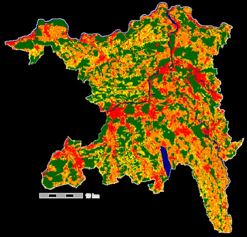
tories included e.g. the Reuss valley (Southeast of the canton, arrow 1 in Figure 8), or the
Lake Hallwil (South, arrow 2 in Figure 8). A contiguous modelled amphibian biodiversity
hotspot can be found along the Aare river (West, arrow 3). It is covered by the "wetland"
REN network, but not by a BLN. In the Southwest of the Canton (arrow 4), modelled bio-
diversity hotspots are partly encompassed by REN areas, but no major BLN is found. This
region of biodiversity hotspots in the reference scenario overlaps with areas, where at least
two future land-use scenarios agreed on predicting biodiversity hotspot losses (Figure 5).
ETH Zürich - Master’s thesis 17Lucie Roth, 31 March 2021 Figure 8: Modelled biodiversity hotspot areas (overlaps of at least seven predicted am- phibian occurrences) of the reference scenario and their overlap with existing landscape inventories (BLN and the "wetland" network of the REN). The arrows highlight the following areas: 1) in the Reuss valley and 2) the Lake Hallwil there is an overlap between high bio- diversity areas and the landscape inventories. 3) Along the Aare river, a large contiguous modelled biodiversity hotspot can be found that is covered by the REN but not by a BLN. 4) In the Southwest of the Canton (regions of Zofingen, Aarau, and Unterkulm), biodiversity hotspots and REN can be found, but no BLN. Map sources: BLN (BAFU 2017c) and REN (BAFU 2011) ETH Zürich - Master’s thesis 18
Lucie Roth, 31 March 2021

4. Discussion
4.1. Model Assessment
All evaluation values indicated a better model performance than random ones and high
spatial agreement between the real and predicted presences. Based on this, the models
were assumed to be robust enough to predict species presence in the study area.

4.2. Effects of future land-use scenarios on amphibian biodiversity
     hotspots
The three scenarios that showed strongest urbanization on the expense of agricultural land
(A2, B2 and Trend, Figures 2 and A.6) were also characterized by the highest losses in
biodiversity hotspot areas (Figure 5). Areas with biodiversity hotspot loss had a higher in-
crease of surrounding urban percentage than gain areas (Table 3). Urbanization could be
confirmed as an important driver of amphibian biodiversity loss, which was also observed
by e.g. Scheffers and Paszkowski (2012). Therefore, my initial hypothesis that scenarios
predicting on the one hand high growth of population and economy and on the other hand
have low support of governmental interventions could only be partly confirmed: urban-
ization associated with population growth was affirmed as an important driver, while the
degree of intervention seemed to be less important, as A2 was modelled with "less inter-
vention" and B2 with "more intervention" (Figure 2a). The degree of intervention mainly
influences conservation and agricultural subsidies. For the two agricultural land uses, no
clear trends could be derived (Table 3). This might have resulted from the missing response
of modelled occurrence probabilities on changing values of surrounding agricultural cov-
erage of most species (Figure A.12). Agricultural land uses can have both positive and
negative influences on amphibians (Table 2), which could be a possible explanation for the
observed unclear trend. Knutson et al. (2004) describes agricultural ponds as important
secondary habitats. However, this benefit might be outweighed by the adverse effects of
high levels of nutrients and pesticides (Brühl et al. 2013).
I did not expect that biodiversity hotspot gains and losses contributed nearly equally to the
total predicted change (Figure 5). The analysis of the future urban areas that additionally
showed changes in biodiversity hotspots provided possible starting points for explanations.
According to the results in section 3.2.2, gains in species distributions on future urban-
ized areas can occur, provided that the surrounding coverage of forests is high (median
was > 20 %) and the urban coverage low (median < 70 %, see Figure A.9). These values
could serve as coarse thresholds for the planning of BGI regions. Forested areas provide
important summer and hibernation habitats for many species (Table 1). An increasing per-
centage of forest in the surrounding of a breeding pond was shown to support a higher
larval amphibian species richness (Rubbo and Kiesecker 2005). A high degree of urban ar-
eas usually indicates a high fragmentation and a low probability of suitable habitats (Parris
(2006), Scheffers and Paszkowski (2012)). Additional insight on the biodiversity gain areas
was provided through the analysis where urbanization occurred (Figures 6 and A.6). On
average, urbanization occurred mostly along the river valleys, with a low standard devia-
tion of elevation, and moderate soil moisture values. Consequently, the species gained in
biodiversity hotspot areas mostly in areas with a larger distance to water, a higher standard
deviation of elevation, and lower soil moisture. However, the response curves (Figure A.12)
indicate lower suitability of these areas. Therefore, urbanization seems to reinforce a trend
stated by Flory (1999): Primary, well-suited habitats of the amphibians in the river plains
of the Canton are destroyed which forces amphibians to colonize less suited, secondary
habitats on steeper slopes further away from the river plains. However, the maintenance
of these secondary habitats requires large efforts. For the long-term conservation of the
amphibians, the renaturation of primary habitats is of uttermost importance (Flory 1999).
The finding that losses and gains in biodiversity hotspot areas in all scenarios - even the
ones with the highest risk of urbanization - are almost equally high, is desirable for the fu-
ture conservation of amphibian species in the study area as no drastic decrease in the total

ETH Zürich - Master’s thesis                                                               19
You can also read