A new method (M3Fusion v1) for combining observations and multiple model output for an improved estimate of the global surface ozone distribution ...
←
→
Page content transcription
If your browser does not render page correctly, please read the page content below
Geosci. Model Dev., 12, 955–978, 2019
https://doi.org/10.5194/gmd-12-955-2019
© Author(s) 2019. This work is distributed under
the Creative Commons Attribution 4.0 License.

A new method (M3Fusion v1) for combining observations and
multiple model output for an improved estimate of the global
surface ozone distribution
Kai-Lan Chang1,2,3 , Owen R. Cooper2,3 , J. Jason West4 , Marc L. Serre4 , Martin G. Schultz5 , Meiyun Lin6,7 ,
Virginie Marécal8 , Béatrice Josse8 , Makoto Deushi9 , Kengo Sudo10,11 , Junhua Liu12,13 , and Christoph A. Keller12,13,14
1 National Research Council Research Associateship Program, David Skaggs Research Center, Boulder, CO, USA
2 NOAA    Earth System Research Laboratory, Boulder, CO, USA
3 Cooperative Institute for Research in Environmental Sciences, University of Colorado, Boulder, CO, USA
4 Department of Environmental Sciences & Engineering, University of North Carolina, Chapel Hill, NC, USA
5 Jülich Supercomputing Centre (JSC), Forschungszentrum Jülich, Jülich, Germany
6 NOAA Geophysical Fluid Dynamics Laboratory, Princeton, NJ, USA
7 Program in Atmospheric and Oceanic Sciences, Princeton University, Princeton, NJ, USA
8 Météo-France, Centre National de Recherches Météorologiques, Toulouse, France
9 Meteorological Research Institute (MRI), Tsukuba, Japan
10 Graduate School of Environmental Studies, Nagoya University, Nagoya, Japan
11 Japan Agency for Marine-Earth Science and Technology (JAMSTEC), Yokosuka, Japan
12 NASA Goddard Space Flight Center, Greenbelt, MD, USA
13 Universities Space Research Association, Columbia, MD, USA
14 John A. Paulson School of Engineering and Applied Science, Harvard University, Cambridge, MA, USA

Correspondence: Kai-Lan Chang (kai-lan.chang@noaa.gov)

Received: 19 July 2018 – Discussion started: 5 September 2018
Revised: 30 January 2019 – Accepted: 14 February 2019 – Published: 12 March 2019

Abstract. We have developed a new statistical approach            ozone field to each model in each world region. This method
(M3 Fusion) for combining surface ozone observations from         allows us to produce a global surface ozone field based on
thousands of monitoring sites around the world with the out-      TOAR observations, which we then use to select the com-
put from multiple atmospheric chemistry models to produce         bination of global models with the greatest skill in each of
a global surface ozone distribution with greater accuracy than    eight world regions; models with greater skill in a particular
can be provided by any individual model. The ozone observa-       region are given higher weight. This blended model product
tions from 4766 monitoring sites were provided by the Tro-        is bias corrected within 2◦ of observation locations to pro-
pospheric Ozone Assessment Report (TOAR) surface ozone            duce the final fused surface ozone product. We show that our
database, which contains the world’s largest collection of sur-   fused product has an improved mean squared error compared
face ozone metrics. Output from six models was provided           to the simple multi-model ensemble mean, which is biased
by the participants of the Chemistry-Climate Model Initia-        high in most regions of the world.
tive (CCMI) and NASA’s Global Modeling and Assimilation
Office (GMAO). We analyze the 6-month maximum of the
maximum daily 8 h average ozone value (DMA8) for rel-
evance to ozone health impacts. We interpolate the irregu-
larly spaced observations onto a fine-resolution grid by using
integrated nested Laplace approximations and compare the

Published by Copernicus Publications on behalf of the European Geosciences Union.
956                                                                     K.-L. Chang et al.: Global surface ozone data fusion

1   Introduction                                                   sult, especially if the overall number of ensemble members
                                                                   is small.
Tropospheric ozone is a pollutant detrimental to human                Combining model ensembles using a method more so-
health and has been associated with a range of adverse car-        phisticated than the simple average is a challenge because
diovascular and respiratory health effects due to short-term       a meaningful model evaluation can rarely be condensed into
and long-term exposure (World Health Organization, 2005;           a single metric, and there is no technique that can explic-
Jerrett et al., 2009; US Environmental Protection Agency,          itly quantify the degree of similarity (i.e., both accuracy and
2013; GBD, 2015; Turner et al., 2016; Cohen et al., 2017).         precision) between two different spatial fields (Hyde et al.,
Assessing the human health impacts of ozone on the global          2018). Indeed, Stainforth et al. (2007) concluded that any at-
scale requires accurate exposure estimates at any given in-        tempt to assign weights is, in principle, inappropriate. With
habited location (Shaddick et al., 2018). Due to the lim-          a lack of appropriate criteria, the model weighting approach
ited availability of surface ozone observations in many re-        has not become a standard alternative to the ensemble aver-
gions of the world (Fleming et al., 2018), global atmospheric      age. Accordingly, there is presently no objective criterion for
chemistry models are required to calculate surface ozone           combining surface ozone estimates from a model ensemble
exposure. Despite continual development and improvement,           to produce a surface ozone product with improved accuracy
global models struggle in their ability to accurately simulate     beyond that of any ensemble member or the simple ensemble
ozone in all regions of the world (Young et al., 2018). The        mean. The absence of such a methodology is the motivation
ability to accurately simulate observed ozone at a particular      for this paper.
location also varies between models, as demonstrated by sev-          This paper presents a new statistical approach (M3 Fusion)
eral multi-model comparisons (Stevenson et al., 2006; Young        for combining surface ozone output from multiple atmo-
et al., 2013; Cooper et al., 2014).                                spheric chemistry models with all available surface ozone
   A useful endeavor for producing an accurate representa-         observations to produce a global surface ozone distribution
tion of the global surface ozone distribution is to combine the    with greater accuracy than the multi-model ensemble mean.
output from many models in a way that takes advantage of           As described in greater detail below, this fused surface ozone
the strengths of each model and minimizes the weaknesses.          product is constructed in three steps: (1) ozone observations
Such efforts have already been made for both climate and           from all available surface ozone monitoring sites around the
chemistry–climate models. For example, multi-model output          world are spatially interpolated to a smooth global field;
has been combined using a parametric approach, either by as-       (2) for each of eight continental regions of the world, six
signing an equal or optimum weight to each model (Steven-          global atmospheric chemistry models are evaluated against
son et al., 2006; He and Xiu, 2016; Braverman et al., 2017)        the interpolated observed ozone field by a quadratic program-
or by tuning the initial conditions under different scenarios or   ming optimization, with the most accurate models receiving
parameterizations (Cariolle and Teyssèdre, 2007; Wu et al.,        the highest weight; a locally confined spline interpolation
2008; Young et al., 2013). These approaches often assume           is used at the regional boundaries to avoid unphysical step
that individual model biases will at least partly cancel by av-    changes; (3) finally, the global ozone field derived from the
eraging or weighting, according to certain measures of pre-        polynomial equation is bias corrected but only within a lim-
dictive performance. Thus, the combined model product is           ited distance from available observations. The final product is
likely to be more accurate than a single model prediction,         based on the annual maximum of the 6-month running mean
as has been shown for multi-model combinations of past or          of the monthly average daily maximum 8 h average mixing
present-day climate (Buser et al., 2009; Knutti et al., 2010;      ratios (DMA8), a metric that can be used to estimate human
Weigel et al., 2010; Chandler, 2013).                              mortality due to long-term ozone exposure (Turner et al.,
   For the case of simply averaging the output from multi-         2016; Malley et al., 2017; Seltzer et al., 2018; Shindell et al.,
ple climate models, most studies either explicitly or implic-      2018).
itly assume that every model is independent and is a random           Past estimates of global mortality due to long-term ozone
sample from a distribution, with the true climate as its un-       exposure have relied on surface ozone fields produced by
biased mean. This implies that the average of a set of mod-        global atmospheric chemistry models due to the limited cov-
els converges to the true climate as more and more models          erage of the global ozone monitoring network (Anenberg
are added. This multi-model ensemble often outperforms any         et al., 2010; Brauer et al., 2012, 2015; Malley et al., 2017).
single model in terms of the predictive capability. Undeni-        The fused surface ozone product is a blend of global surface
ably, when one has several dozen or hundreds of possible           ozone observations and model output that has been adjusted
ensemble members, the most straightforward and efficient           according to the observations. This particular product will be
approach is to simply take the ensemble average, ignoring          available for future estimates of global human mortality due
the impact of potentially erroneous outlier ensemble mem-          to long-term ozone exposure (e.g., Global Burden of Disease,
bers. From a statistical point of view, one might argue that       Brauer et al., 2012, 2015). Furthermore, the methodology can
ruling out potentially erroneous ensemble members prior to         be applied to a range of ozone metrics for quantifying the im-
conducting the ensemble mean would yield an even better re-

Geosci. Model Dev., 12, 955–978, 2019                                                 www.geosci-model-dev.net/12/955/2019/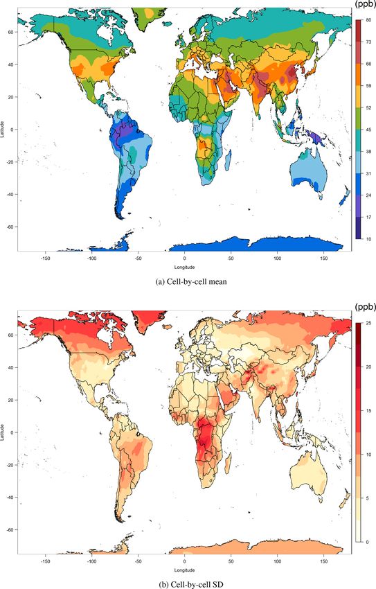
K.-L. Chang et al.: Global surface ozone data fusion                                                                            957

pacts of ozone on human health, or vegetation, and it can also           by Turner et al. (2016) to quantify the impact of long-
be applied to PM2.5 , CO2 or any other trace gas.                        term ozone exposure on human mortality. Hereinafter,
   Section 2 provides details of the data sources and fusion             this quantity is simply referred to as “the ozone metric”.
process, including the techniques to register all data sources
onto a common grid and the statistical model used to min-            2. Atmospheric chemistry model simulations. We use out-
imize the difference between interpolated observations and              put from models from phase 1 of the Chemistry-
the multi-model combination. In Sect. 3, the results of em-             Climate Model Initiative (CCMI), downloaded from
ploying these techniques are presented, including the map-              the Centre for Environmental Data Analysis (CEDA)
ping accuracy, evaluation of regional model performance and             database (http://archive.ceda.ac.uk, CEDA, 2019). We
the final multi-model bias correction. The paper concludes              chose four models (CHASER, GEOSCCM, MOCAGE
with a summary and discussion in Sect. 4.                               and MRI-ESM1r1) because they report hourly ozone
                                                                        output (Table 1). These particular simulations were part
                                                                        of CCMI’s REF-C2 experiment (Morgenstern et al.,
2     Data and method                                                   2017), which follows the World Meteorological Orga-
                                                                        nization (2011) A1 scenario for ozone depleting sub-
2.1    Observations and model output                                    stances, and RCP6.0 for tropospheric ozone precur-
                                                                        sors, and aerosol and aerosol precursor emissions (Mor-
    1. Tropospheric Ozone Assessment Report (TOAR) surface              genstern et al., 2010) for the period 1960–2100. Even
       ozone database. In this analysis, surface ozone observa-         though the most appropriate experiment would have
       tions are used to evaluate the performance of six global         been the REF-C1SD, in which the models are nudged to
       atmospheric chemistry models and to also bias correct            the reanalysis meteorology and thus best represent the
       the multi-model surface ozone product. TOAR has pro-             past in the observations, we use output from the REF-
       duced the world’s largest database of surface ozone met-         C2 simulation in this study, as the last year of the REF-
       rics based on hourly observations at over 9000 sites             C1SD was 2010 and would therefore not cover the most
       around the globe (Schultz et al., 2017, ozone met-               recent period where observations are available. How-
       rics available for download at https://doi.org/10.1594/          ever, the NOAA Geophysical Fluid Dynamics Labora-
       PANGAEA.876108). Spatial coverage is high in North               tory (GFDL) AM3 model continued the simulation over
       America, Europe, South Korea and Japan, but much                 the entire study period and was therefore selected for
       lower across the rest of the world with very low data            this analysis. In addition, we obtained output from the
       availability across Africa, the Middle East, Russia and          GEOS-5 nature run with chemistry (G5NR-Chem), pro-
       India. In addition to data sparseness, other challenges,         vided by the NASA Global Modeling and Assimilation
       such as data inhomogeneity in time and the irregu-               Office (GMAO), which we included in our analysis be-
       lar spatial distribution of stations (Chang et al., 2017),       cause of the model’s very fine horizontal resolution (Hu
       make the comparison between model output and ob-                 et al., 2018), but the output was only available for July
       servations difficult without serious statistical modeling.       2013 to June 2014.
       While satellite retrievals have been utilized by previ-
                                                                         The output from each individual model is shown in
       ous works for quantifying the health impacts of PM2.5
                                                                         Fig. S1 in the Supplement. Note that NASA G5NR-
       (Brauer et al., 2012, 2015), satellite retrievals of tro-
                                                                         Chem has the finest resolution of these models; accord-
       pospheric ozone have limited sensitivity near the sur-
                                                                         ingly, we aim to produce our final product on the same
       face and are inadequate for this analysis (Gaudel et al.,
                                                                         0.125◦ × 0.125◦ grid. However, even at this resolution,
       2018).
                                                                         the output is not street resolving and thus will not cap-
       TOAR has gathered ozone observations through 2014 at              ture urban-scale variability in the regions with the high-
       most sites and has chosen 2008–2014 as a “present-day”            est population density.
       window for more rigorous analysis. The purposes of the
       multi-year average are to reduce the effects of ozone in-       In order to compare model output to observations, we
       terannual variability, which is largely driven by changes    need to register model output and observations to a com-
       in meteorological conditions (Strode et al., 2015), and      mon grid. This registration enables us to quantify the dif-
       to increase the number of available sites than if we used    ferences between the models and observations. Previous at-
       a single year. In this analysis, we focus on the annual      tempts have usually relied on a variant from a general statisti-
       maximum of the 6-month running mean of the max-              cal interpolation framework to combine incompatible spatial
       imum daily 8 h average (DMA8) at every site in the           data (Gotway and Young, 2002; Fuentes and Raftery, 2005;
       TOAR database. Specifically, the metric was calculated       Gelfand and Sahu, 2010; Berrocal et al., 2012; Nguyen et al.,
       from the 6-month running mean of the monthly mean            2012). Due to the highly irregular locations of ozone mon-
       DMA8 ozone values at a given site. This metric was           itors around the globe, we use a kriging technique to build
       selected because it aligns with the ozone metric used        a statistical model, interpolate the ozone distribution based

www.geosci-model-dev.net/12/955/2019/                                                    Geosci. Model Dev., 12, 955–978, 2019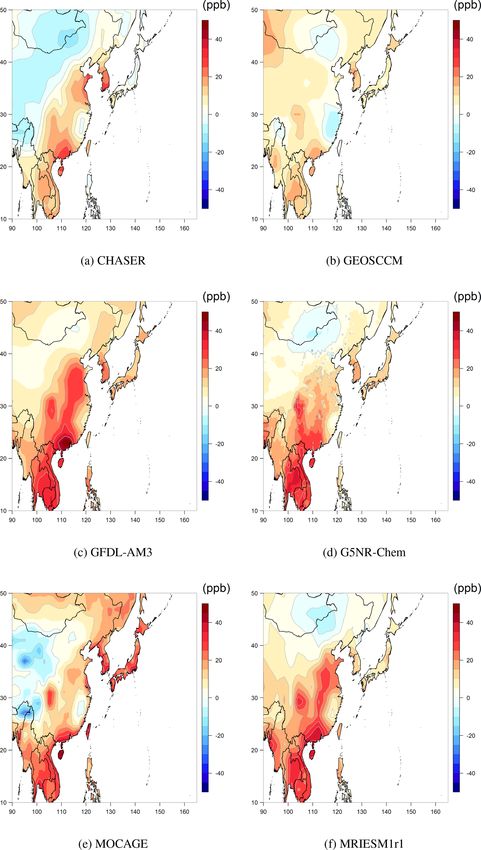
958                                                                                                 K.-L. Chang et al.: Global surface ozone data fusion

Table 1. List of the ensemble members used in this paper.

   Model ID               Group                                                                Resolution              Meteorological        References
                                                                                                                       Forcinga
   CHASER                 Nagoya University; Japan Agency for Marine-Earth                     2.8◦ × 2.8◦             C2                    Sudo et al. (2002a, b),
   (MIROC-ESM)            Science and Technology (JAMSTEC), Japan                                                                            Watanabe et al. (2011)
   GEOSCCM                NASA Goddard Space Flight Center, USA                                2.5◦ × 2◦               C2                    Oman et al. (2011)
   GFDL-AM3               NOAA Geophysical Fluid Dynamics Laboratory, USA                      2◦ × 2◦                 C1SD                  Lin et al. (2012, 2014, 2017)
   G5NR-Chem              NASA Goddard Space Flight Center, USA                                0.125◦ × 0.125◦         b                     Hu et al. (2018)
   MOCAGE                 Centre National de Recherches Météorologiques;                       2◦ × 2◦                 C2                    Josse et al. (2004),
                          Météo-France, France                                                                                               Teyssèdre et al. (2007)
   MRI-ESM1r1             Meteorological Research Institute, Japan                             2.8◦ × 2.8◦             C2                    Adachi et al. (2013)
a Meteorological forcing includes coupled ocean–atmosphere (C2) and nudged to observed reanalysis meteorology (C1SD) in CCMI reference simulations (Morgenstern et al., 2017).
b The specification of forcing scenario for this special run is described by Hu et al. (2018).

on the surrogate and then project the global surface onto a                                  model product evaluated by the interpolated ozone observa-
common grid.                                                                                 tions. We propose the following procedure to combine model
                                                                                             output and observations for data integration:
2.2     Fusion of observations and models
                                                                                                1. Interpolating irregularly located monitoring observa-
Following is a description of our method for fusing obser-                                         tions to the model output grid. Kriging is a proce-
vations and output from multiple global atmospheric chem-                                          dure used to statistically interpolate irregularly spaced
istry models to produce a surface ozone product with maxi-                                         and/or sparse observed data onto a regular and dense
mized accuracy. This method is known as Measurement and                                            grid, based on a weighted average of the fitted surrogate
Multi-Model Fusion (version 1), or M3 Fusion (v1), and the                                         model in the neighborhood of the grid. We assume that
code accompanies this paper in the Supplement. We consider                                         the global ozone distribution can be approximated by
a general framework of uncertainty quantification consisting                                       a Gaussian spatial process (GP) with a constant mean
of the following components (Kennedy and O’Hagan, 2001;                                            and Matérn covariance function (Stein, 2012). The GP
Chang and Guillas, 2019):                                                                          fitting typically involves a cubic complexity and thus
                                                                                                   is computationally expensive for large spatial data sets.
observation = reality + random error;
                                                                                                   Therefore, several alternatives have been developed to
       reality = model + structured bias.                                                          address the large n issue by using a reduced set of data
Since this equation requires matching components (observa-                                         (Cressie and Johannesson, 2008; Banerjee et al., 2012;
tions and model output) on a common grid, we use the in-                                           Liang et al., 2013), tapering the covariance between two
terpolated observations to estimate an optimized weight for                                        grid points to zero if their distance is beyond a certain
each model by a L2 norm (details are given later), which                                           range (Furrer and Sain, 2009; Sang and Huang, 2012)
means that we expect the multi-model combination to cap-                                           and/or evaluating the covariance only through the spec-
ture the general pattern of the surface ozone distribution in                                      ification of a neighborhood system (also known as the
terms of their joint predictive capability, and the model bias                                     Gaussian Markov random field) (Rue et al., 2009; Lind-
is considered as a model correction term. The difference be-                                       gren et al., 2011).
tween observation error and model bias is that the former                                           In this study, we carry out the spatial interpolation by
term is assumed to be a normal noise with zero mean and                                             using the combination of the integrated nested Lapla-
constant variance, and the latter term is considered as a sys-                                      cian approximation (INLA) framework (Rue et al.,
tematic and structured discrepancy (Williamson et al., 2015),                                       2009) and the stochastic partial differential equation
which will be revealed as a spatial cluster across a poorly                                         (SPDE) technique (Lindgren et al., 2011), available as
simulated region.                                                                                   an R package (http://www.r-inla.org/) (Lindgren and
   Due to this study’s human health focus, we do not consider                                       Rue, 2015). The details of this technique are rather
ozone above the data-sparse oceans. Above land, large ob-                                           complex and the reader is referred to the original pa-
servational gaps are present across Africa, the Middle East,                                        per (Lindgren et al., 2011); however, we describe the
South America, and south and southeast Asia, where the spa-                                         key component of this INLA-SPDE technique in Ap-
tial interpolation is generally too uncertain to yield a reli-                                      pendix A. INLA-SPDE spatial modeling has proven to
able surface ozone approximation. The ozone estimates in                                            be effective in a wide range of applications (Cameletti
these regions must come from either models or distant ob-                                           et al., 2013; Shaddick and Zidek, 2015; Heath et al.,
servations, neither of which is ideal to solve this issue. As                                       2016; Liu and Guillas, 2017; Rue et al., 2017). We
a compromise strategy, we fill these gaps with a weighted                                           chose this technique because it manages a fairly large

Geosci. Model Dev., 12, 955–978, 2019                                                                                   www.geosci-model-dev.net/12/955/2019/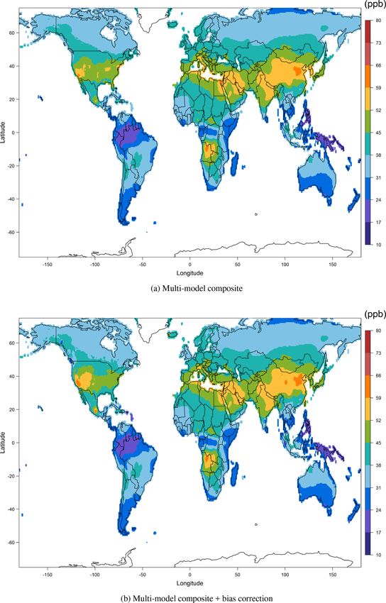
K.-L. Chang et al.: Global surface ozone data fusion                                                                                                  959

    and complex spatial field in a relatively efficient way        squares approach:
    (Rue and Held, 2005) and allows an extension for non-                                                                                    !2
                                                                                                                           6
    stationarity on the sphere (Bolin and Lindgren, 2011;             minimize
                                                                                              X
                                                                                                          ŷ(sg ) − αr −
                                                                                                                           X
                                                                                                                                 βr k ηk (sg )    ,   (1)
    Chang et al., 2015). Notably, a recent study elaborately       {αr ,βr k ;k=1,...,6}
                                                                                           sg ∈Region r                    k=1
    compared dozens of spatial modeling approaches, and                              6
                                                                                     X
    the results suggest that almost all of these approaches        subject to                 βr k = 1 and βr k ≥ 0.,
    can achieve a similar performance in terms of their pre-                         k=1
    dictive accuracy, albeit with very different computation
                                                                   where αr is a constant that allows adjustment to the
    times (Heaton et al., 2018). Therefore, we expect that
                                                                   overall (regional) underestimation or overestimation;
    the choice of spatial modeling approach is not the most
                                                                   βr k is an optimal weight for the kth model in region r.
    crucial component in our data fusion process as long
                                                                   Note that since the interpolated observations and mod-
    as the analysis is carried out in a rigorous way (i.e.,
                                                                   els use the same ozone metric with the same units, we
    through the statistical model selection and diagnostics).
                                                                   constrain the weights to be positive and sum to 1 for a
    To differentiate this result from the actual observations
                                                                   better physical interpretability, such that the most accu-
    in the TOAR database, we refer to this interpolated sur-
                                                                   rate models receive the higher weight. The offset term
    face as the “spatially interpolated ozone”.
                                                                   αr is aimed to adjust the overall residuals between the
    We carry out the statistical interpolation via the fol-        observation field and the multi-model composite into
    lowing steps: (1) calculate the ozone metric at each           zero mean in each region (regardless of the spatial pat-
    TOAR site and for every year in 2008–2014; (2) per-            tern); therefore, if two spatial fields share a great simi-
    form the statistical interpolation using all available sites   larity in terms of their spatial curvatures, but the overall
    with their exact coordinates and project the surface           means are different, this term can fill the gap of the over-
    onto a 0.125◦ × 0.125◦ spherical grid for every year;          all mean difference between the two fields. The weights
    (3) average these surfaces over the 7 years to yield an        are optimized in terms of the squared distance between
    observation-based present-day ozone distribution. We           the interpolated ozone and multi-model output. A dif-
    expect that this aggregation will smooth out at least          ferent criterion of optimization, such as mean absolute
    some of the potential uncertainties. The kriging can be        error, can be established accordingly.
    seen as a nonparametric regression problem; therefore,         Due to the sparsity of stations in many regions, we
    a statistical assessment of fitted quality must be consid-     use a predefined geometric boundary to differentiate re-
    ered to select the best representation to the data (Hoet-      gions. A more meaningful physical boundary (i.e., re-
    ing et al., 2006). Further details on the statistical model    gions with similar chemical regimes or major features
    selection procedure are provided in Appendix A.                such as deserts, mountain ranges or water bodies) might
    We use a bilinear interpolation to smooth model out-           be determined using a cluster analysis technique (Hyde
    put from coarser resolution to a 0.125◦ × 0.125◦ grid          et al., 2018), but such a step is beyond the scope of this
    (Jun et al., 2008). The ozone metric for each model was        paper.
    calculated for each single grid in each year, then aver-       Since we partition the global land surface into eight re-
    aged over 2008–2014 (except for NASA G5NR-Chem,                gions and evaluate the models individually, inevitably
    which was already in fine resolution, but only available       there will be disjointed boundaries between regions.
    for 1 year).                                                   The boundaries between North and South America,
                                                                   or between east Asia and Oceania, fall mostly in the
 2. Weighting model output against spatially interpolated          oceans, so we do not need to adjust these regions.
    ozone by region. The next step is to create an intermedi-      However, we should make an adjustment to disjointed
    ate “multi-model composite”. We divide the global land         boundaries that fall across inhabited areas (see Fig. S2
    surface into eight regions (see Fig. 1), roughly match-        for the illustration). As an example of our method, con-
    ing the continental outlines or major population regions.      sider the boundary between east Asia and Russia near
    We adopt this regional approach because global models          50◦ N. We increase the northern boundary of east Asia
    vary in their ability to simulate ozone in different re-       to 55◦ N and decrease the southern boundary of Rus-
    gions of the world. Next, we regress the observations          sia to 45◦ N, to create an overlapping intersection, and
    on multi-model output by a constrained least square            then fit cubic splines (performed for each grid cell) with
    approach within each of the eight regions. Let sg be           knots placed at every 2◦ grid cell (Wood et al., 2008).
    the grid cell at resolution 0.125◦ × 0.125◦ , ŷ(sg ) be the   This smoothing is carried out using a low-rank Gaus-
    interpolated observations and {ηk (sg ); k = 1, . . ., 6} be   sian process by the default penalized least square from
    the model output registered onto the same grid from            the function “gam” in the R package mgcv (Kammann
    the six models considered in this paper (Table 1). The         and Wand, 2003; Wood, 2017), following the exam-
    optimization equation is based on a constrained least          ples of Wood and Augustin (2002). The purpose is to

www.geosci-model-dev.net/12/955/2019/                                                         Geosci. Model Dev., 12, 955–978, 2019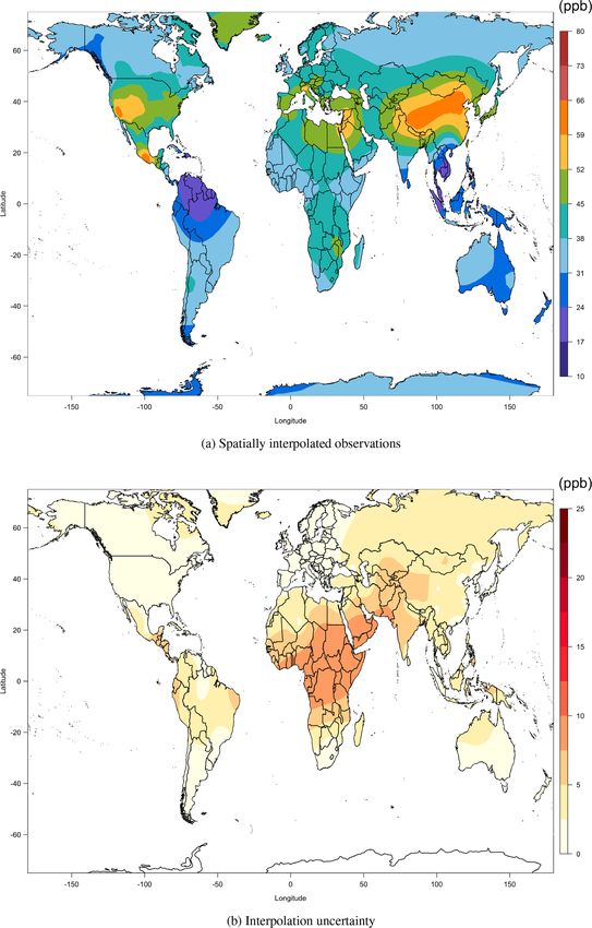
960 K.-L. Chang et al.: Global surface ozone data fusion
merely avoid a sharp and unrealistic (geometric) tran- from correcting the model in these regions. Instead, we
sition between three regions and to efficiently smooth conduct a limited model bias correction based on the
out the discontinuity, performed in a regular spaced grid distance to the nearest monitoring station, but we ignore
only around the geometric boundary. Any region away the differences between the multi-model composite and
from the geometric boundary will not be affected by this the interpolated observations in the sparsely monitored
smoothing, which should be considered as a blending of regions. In our approach, we only correct the output grid
multiple models without any attempt of bias correction. where there is at least one observational station within
It should be noted that the INLA-SPDE technique in a 2◦ radial distance of the grid cell in question (i.e., the
step 1 is applied to the observations, while the smooth- distance to the nearest station is less than 2◦ ). We then
ing spline is only applied to the boundaries between re- end up using
gions of the model composite, not directly involving any
ŷ(sg ), if a grid cell sg is within a 2◦ radial distance
observations.
of the station;
We adopted a regression weighting approach that only
6
accounts for the mean spatial fields of the interpo- αr +
P
βr k ηk (sg ), otherwise,
lated ozone and model output, rather than the underly- k=1
ing associated uncertainty. We take this approach due
to the prohibitive size of high-resolution output (over to generate our high-resolution global surface ozone es-
1 million output points for each model) but also due timate. Given the limited availability of observations
to the lack of a thorough investigation regarding the worldwide, we were only able to apply this final bias
ideal method for combining models based on different correction to 14.4 % of the globe’s land area. We refer to
sources of uncertainty. For example, the interpolation the final outcome as the “fused surface ozone product”.
uncertainty can be quantified easily through the poste-
rior distribution and considered to be related to mea-
surement error (small scale) or sparse sampling across 3 Results
a region (large scale); however, model uncertainty is a
different concept altogether that could result from input 3.1 Mapping and uncertainty
uncertainty (e.g., air pollution emissions inventories) or
limitations of the transport and chemistry mechanisms Ground-based measurements were available from 4766 sta-
within the model (Brynjarsdóttir and O’Hagan, 2014). tions reported in the TOAR database (Schultz et al., 2017).
The current interest of this study focuses on a better To illustrate the spatial coverage of the database, Fig. 1 shows
estimate of mean ozone exposure. Explicit quantifica- the ozone metric discretized to a 2◦ × 2◦ grid (a finer resolu-
tion of different sources of model uncertainty and in- tion will be too obscure for illustrative purposes), averaged
corporation of this information into the data fusion pro- over the period 2008–2014. This figure also shows our re-
cess presents another level of complexity that cannot be gionalized classification, including Africa, North America,
tackled until model uncertainties are better character- South America, east Asia, southeast and central Asia, Eu-
ized. Young et al. (2018) provide a current overview of rope, Oceania and Russia. Note that dense station networks
chemistry–climate modeling and discuss the challenges are found in North America, Europe and east Asia (mostly
of improving models in light of so many uncertainties. in Japan and South Korea), while monitoring sites are more
widely scattered across the remaining regions. The highest
3. Correcting multi-model bias in areas close to observa- average ozone levels are found at sites in China, South Korea,
tions. A common practice of studying the model dis- Japan, Taiwan, India, Greece, California and Mexico City.
crepancy in the spatial fields is to fit a statistical model Figure 2a shows the spatially interpolated surface in each
for their differences from observations on the whole cell. For each grid cell, there is an underlying (poste-
spatial domain, to see whether or not these residuals re- rior) probability distribution which incorporates information
veal any structured spatial pattern (Jun and Stein, 2004; about the interpolation uncertainty. Figure 2b shows the half
Sang et al., 2011). If the model adequately simulates the width of the 95 % posterior credible interval in each cell
ozone distribution (up to a level shift and a scale factor), (Shaddick et al., 2018). From the spatial pattern of uncer-
then there is no relevant information in these residuals. tainty, we can see that relatively higher uncertainties are ex-
On the other hand, if the model does not properly repre- pected in Africa, the Middle East, south Asia and Russia,
sent the local structure, then the residuals should exhibit regions with very limited observations; lower uncertainty is
a signal of the discrepancy in that region (Guillas et al., associated with regions with a dense station network, such
2006; Williamson et al., 2015). However, in our case, as North America and Europe. Due to the limitations of spa-
the regular grid observation field is obtained from spa- tial kriging in a sparsely monitored region, the observations
tial kriging, such that in many data-sparse regions we are often interpolated across very great distances, such as in
do not actually have observed ozone, which prevents us South America, Africa and central Asia. This method is not
Geosci. Model Dev., 12, 955–978, 2019 www.geosci-model-dev.net/12/955/2019/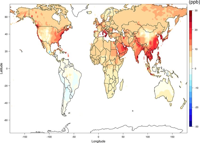
K.-L. Chang et al.: Global surface ozone data fusion                                                                                 961

Figure 1. TOAR observations where the monitoring locations are discretized to a 2◦ × 2◦ grid in 2008–2014.

ideal, and instead information from models can be used to fill        more detailed structure in regions with a dense station net-
in the blanks.                                                        work. In contrast, the multi-model mean is more noisy. Even
   The ozone metric for each model was calculated for each            though we average across multiple years and multiple mod-
individual grid cell in each year, then averaged over 2008–           els, the resulting ozone metric can still be noisy because
2014 and registered to the common 0.125◦ ×0.125◦ grid (ex-            it is calculated at each grid cell independently. In order to
cept for NASA G5NR-Chem, which was already in fine res-               make maximum use of the skill of each model, we restrict
olution, but only available for 1 year). Figure 3a shows the          the model evaluation to the regional scale in the next section.
surface ozone metric which results from the simple ensem-
ble average of the six models. It was generated from bilinear         3.2   Regional model evaluation and multi-model
interpolation of the ozone metric on the standard output grid,              composite
by calculating the same metric for each grid cell in each year,
averaging over 2008–2014 and then averaging over the six              To evaluate the performance of each model in a given region,
models. We refer to this product as the “multi-model mean”,           we calculate the mean differences over all grid cells within
and we use it to validate our final product, which should out-        the region and summarize them with the root mean square er-
perform not only each individual model but also the multi-            ror (RMSE). Let ŷ(sg ) be the spatially interpolated observa-
model mean.                                                           tions and {ηk (sg ); k = 1, . . ., 6} be the output corresponding
   Averaging all six models captures the large-scale varia-           to the six ensemble models considered in this paper; then, the
tions of the ozone distribution; however, many regions in             (normalized) RMSE is given by
northern midlatitudes and low latitudes are biased high com-                       s
pared to the observations in the TOAR database. A simple                               P                                    2
                                                                                           sg ∈Region r   ηk (sg ) − ŷ(sg )
approach to address the uncertainty in the multi-model mean           RMSEr k =                                                  ,
is to calculate the standard deviation for each grid cell from                                            n
the different models, as shown in Fig. 3b. Higher model un-           where n is the number of grid cells in a given region r. The
certainties across south Africa and the Middle East match the         first part of Table 2 shows the RMSE statistics for each model
pattern of the interpolation uncertainty in Fig. 2b, and lower        by region. The reliability of such an evaluation is limited by
model uncertainties occur in regions with dense station net-          the station density in a given region, with greater reliabil-
works. These findings suggest that the multi-model mean un-           ity in a dense network (e.g., USA) and less reliability in a
certainty can also reflect the current limited understanding of       sparse network (e.g., Africa, South America or Australia).
surface ozone in regions with limited or no observations.             On average, CHASER, GEOSCCM and G5NR-Chem have
   It should be noted that the spatially interpolated observa-        the lowest biases in multiple regions; GFDL-AM3 and MRI-
tions are smoother in regions with fewer sites and reveal a           ESM1r1 also show low mean biases in certain regions, such

www.geosci-model-dev.net/12/955/2019/                                                         Geosci. Model Dev., 12, 955–978, 2019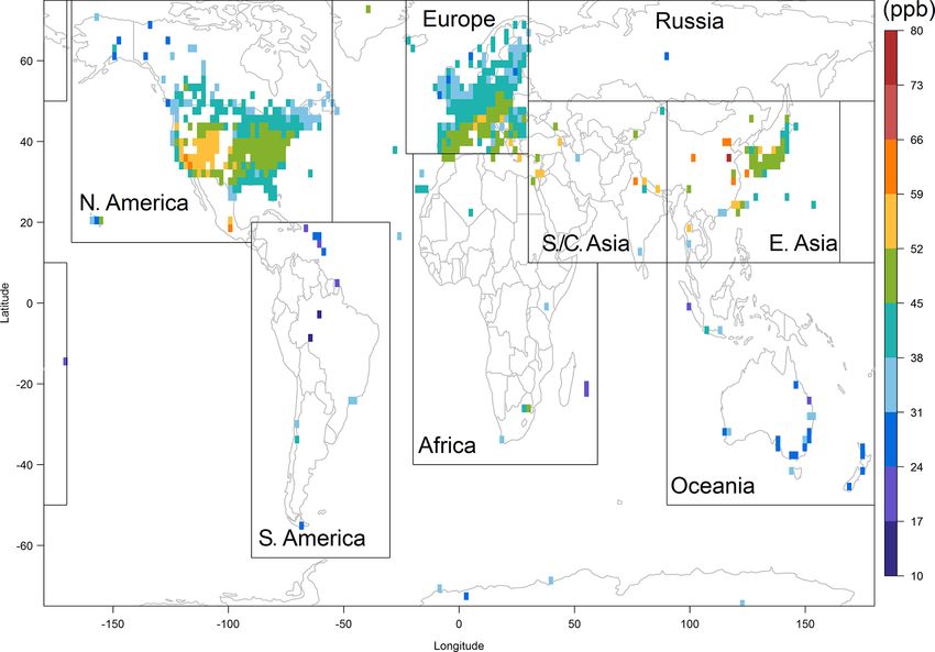
962                                                                           K.-L. Chang et al.: Global surface ozone data fusion

Figure 2. Estimates of spatially interpolated surface ozone distribution and associated uncertainty (half width of the 95 % credible interval
from each cell).

as America and Europe. However, larger model biases can be               and model output in North America. A consistent underes-
found in Africa, and east and south Asia.                                timation can be found in the Mexico City region for all mod-
   Next, we select three regions with extensive monitoring:              els. A clear overestimation is also found across much of the
North America, Europe and east Asia. Figure 4 shows the                  eastern US, as well as the western US and Canada, except
differences between the spatially interpolated observations              for CHASER, which shows a mild underestimation in these

Geosci. Model Dev., 12, 955–978, 2019                                                        www.geosci-model-dev.net/12/955/2019/
K.-L. Chang et al.: Global surface ozone data fusion                                                                             963

Figure 3. Multi-model mean and standard deviation (SD) in each grid cell from six ensemble members.

regions; in Europe (Fig. 5), the models show mild levels of          China, the large scale of these estimated biases might be an
overestimation across most of the region, especially for Italy.      interpolation artifact.
In east Asia (Fig. 6), the models show a major bias across              We argue that the credibility of the model is not en-
east China and a similar bias pattern across the entire region,      tirely decided by the RMSE (i.e., the mean difference): the
although the bias amplitude is smaller for GEOSCCM. How-             smoother the difference plots, the easier it is to carry out the
ever, since the observations are relatively sparse in mainland       model bias correction. Indeed, the observations and model

www.geosci-model-dev.net/12/955/2019/                                                     Geosci. Model Dev., 12, 955–978, 2019
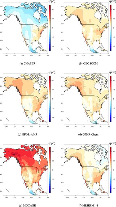
964                                                                          K.-L. Chang et al.: Global surface ozone data fusion

Figure 4. Spatial distributions of the ozone metric in North America from each model minus spatially interpolated observations.

Geosci. Model Dev., 12, 955–978, 2019                                                       www.geosci-model-dev.net/12/955/2019/
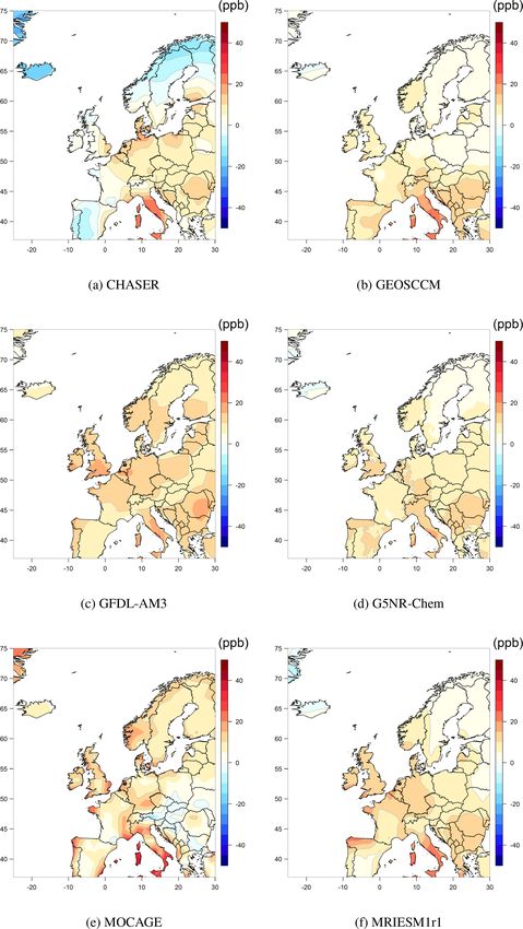
K.-L. Chang et al.: Global surface ozone data fusion                                                                           965

Figure 5. Spatial distributions of the ozone metric in Europe from each model minus spatially interpolated observations.

www.geosci-model-dev.net/12/955/2019/                                                         Geosci. Model Dev., 12, 955–978, 2019
966                                                                           K.-L. Chang et al.: Global surface ozone data fusion

Figure 6. Spatial distributions of the ozone metric in east Asia from each model minus spatially interpolated observations.

Geosci. Model Dev., 12, 955–978, 2019                                                        www.geosci-model-dev.net/12/955/2019/
K.-L. Chang et al.: Global surface ozone data fusion                                                                           967

output are not expected to match point by point. We should         3.3   Local bias correction
also expect the model to capture the general pattern of the
spatial distribution, rather than a pointwise agreement.           The last step of producing the final fused surface ozone
   The estimated weights from the constrained least squares        product is to apply a bias correction to our multi-model com-
(Eq. 1) are given in the second part of Table 2. Due to fixed      posite, limited to just those areas in close proximity to ozone
underlying spatial structures, this approach tends to give         observations. Ideally, we would like to apply a bias correc-
greater weight to a single model (i.e., ≥ 50 %); the one which     tion according to raw observations, but most stations are
provides the best match between its spatial structure and          not exactly located on the model grid coordinates (even at
the observational field (e.g., G5NR-Chem in North Amer-            0.125◦ × 0.125◦ resolution). Therefore, to carry out a statis-
ica). Note that this approach disfavors noisy spatial structure;   tical bias correction on a particular grid, we need to consider
therefore, the algorithm gives low weights to MOCAGE, for          the number of nearby stations and the distance to each sta-
several reasons. First, the MOCAGE ozone field has not been        tion. All these considerations aim to deduce a single correc-
smoothed by interpolation since it is already produced on the      tion value on a single grid, and thus we are still faced with
MOCAGE model grid, whereas all other models are inter-             implementing statistical interpolation. To avoid adding an-
polated. Secondly, MOCAGE uses a more complete tropo-              other level of complexity, we set the final fused product to be
spheric chemical scheme with a larger range of species (77         exactly equal to the spatially interpolated ozone field within
tropospheric species) and has generally a higher reactivity        2◦ of an observation, as the spatially interpolated ozone field
compared to most chemistry–climate models (CCMs) (Voul-            has already accounted for all observations. Due to the global
garakis et al., 2013). Thus, it tends to provide more tempo-       sparseness of observations, about 85 % of model grid cells
ral and spatial variability. Note that our optimization algo-      over land were not affected by this bias correction. After bias
rithm estimates the weights according to the similarity of the     correcting the multi-model composite grid cells within 2◦ of
spatial structures between the interpolated surface and each       a TOAR observation site, an immediate benefit is seen for the
model. In regions with sparse monitoring, the kriged surface       US, Mexico City, Italy and South Korea (see Fig. 7b).
can be greatly affected by a few scattered stations; therefore,       The choice of the correction range, in this case 2◦ , is a ad
we cannot use the resulting weights to evaluate the actual         hoc decision; we also present results with different correction
model performance in these regions.                                ranges in Figs. S3 and S4. When the radius of influence of the
   The last column of Table 2 shows the averaged and com-          TOAR observations is increased to 5◦ or more, the greatest
bined RMSEs from the equal weights and the constrained             impact is seen for the Mexico City region and eastern China.
weights. A reduced overall bias can be generally achieved          An increase of correction range is not ideal because it extrap-
from the constrained weights. This approach suggests that          olates the Mexico City ozone values into the less populated
even if a model has a large mean error (e.g., GFDL-AM3),           regions of Mexico. Increasing the radius to 5◦ or more does
it can still be a good simulation if it produces a spatial pat-    not improve upon the RMSE associated with 2◦ . Therefore,
tern and curvature similar to the observation field. A con-        accepting the 2◦ bias correction over other ranges is subjec-
stant offset αr in the optimization Eq. (1) is included to re-     tive.
move the overall bias over each region, such that the resid-          The fused product can be evaluated in terms of spatial cor-
uals from the optimization have a zero mean. On the other          relation using the variogram which assumes that spatial cor-
hand, if we do not include αr in the equation, GFDL-AM3            relation is not a function of absolute location but only a func-
will have a smaller weight in the optimization, and CHASER,        tion of distance (i.e., stationarity). Since spatial variability
GEOSCCM and G5NR-Chem will dominate most of these                  and continuity from the models are the result of geophysical
regions (not shown).                                               processes represented by mathematical equations, the vari-
   We combine all models according to the optimum weights          ogram must be customized for each field. In addition, the
from each region for each model. Figure 7a shows a map of          extremely large size of the model output prohibits us from
the multi-model composite, a weighted blend of the six mod-        carrying out a standard empirical variogram analysis, which
els, with the weighting calculated separately for each con-        requires calculating the variance of the difference between
tinent. Models with greater simulation skill receive higher        all pairwise grid cells.
weighting. The result reveals a systematic adjustment to              Nevertheless, we provide examples of omnidirectional
the large-scale overestimation from the ensemble mean in           variograms for the spatial field in North America from each
Fig. 3a. This demonstration of a general high bias among           model and product in Fig. S5. The standard variogram analy-
the models argues against using the simple ensemble model          sis focuses on the following three parameters: (1) the nugget
mean for estimating surface ozone. However, when com-              (variance at zero distance, which represents a subgrid vari-
pared to the TOAR observations, the multi-model composite          ation), which is similar for all cases; (2) the sill (total vari-
still has clear local biases.                                      ance of a field), where the variogram value reaches a maxi-
                                                                   mum and levels off; (3) the range (a distance where the sill
                                                                   is reached, and beyond that there is no longer spatial corre-
                                                                   lation). Note that a continuously increasing variogram indi-

www.geosci-model-dev.net/12/955/2019/                                                   Geosci. Model Dev., 12, 955–978, 2019
968 K.-L. Chang et al.: Global surface ozone data fusion Figure 7. Multi-model composite and bias-corrected surface. Geosci. Model Dev., 12, 955–978, 2019 www.geosci-model-dev.net/12/955/2019/
K.-L. Chang et al.: Global surface ozone data fusion                                                                                                  969

Table 2. RMSEs (averaged errors in a given region) between spatially interpolated observations and each model, along with regionally
optimized weights {βrk : for kth model in region r} (zero weights are not displayed). Last column shows the RMSEs from equal weighted
averages or constrained weights from the multi-model composite. All the numbers are reported in units of ppb (i.e., parts per billion by
volume).

      Region                                                  Regional RMSE                                                       Averaged error
                           CHASER       GEOSCCM       GFDL-AM3        G5NR-Chem        MOCAGE             MRI-ESM1r1
      Africa                    6.40           8.91          12.16           12.16            10.47                 14.89                     10.83
      N. America               10.04           8.90          11.28            9.20            24.39                  8.41                     12.04
      S. America                7.39           7.19          10.00            8.81            10.59                  8.59                      8.76
      E. Asia                   9.12           9.42          15.89           13.33            17.68                 14.40                     13.31
      S./C. Asia                7.68          15.11          13.36           13.38            13.37                 18.41                     13.55
      Europe                    9.14           8.41          10.75            8.20            11.88                  9.66                      9.67
      Oceania                   6.00           6.81          11.82            9.42             9.38                  9.24                      8.78
      Russia                    6.59           9.10          11.71            7.86            20.29                  6.04                     10.27
      Region                             Constrained weights of the multi-model composite                                       Composite error
                      αr   CHASER       GEOSCCM       GFDL-AM3        G5NR-Chem        MOCAGE             MRI-ESM1r1
      Africa       −5.25        0.27           0.12           0.43            0.01              0.17                      –                    5.39
      N. America   −7.84           –           0.38              –            0.62                 –                      –                    4.35
      S. America    2.13        0.63           0.13              –            0.24                 –                      –                    5.37
      E. Asia      −7.99        0.08           0.83           0.09               –                 –                      –                    4.88
      S./C. Asia   −8.90        0.52           0.26           0.12            0.10                 –                      –                    4.95
      Europe       −9.91           –              –           0.78            0.13              0.09                      –                    2.75
      Oceania      −2.36        0.73              –              –            0.27                 –                      –                    5.76
      Russia       −7.15        0.21              –           0.45            0.32              0.02                      –                    2.04

cates the evidence of nonstationarity in the field, which is          Table 3. RMSE against TOAR observations (i.e., not interpolated
the case for SPDE, an issue that we have accounted for. The           ozone) from the multi-model mean (MMM), multi-model compos-
variogram peak is about 35–40◦ for the models. The result             ite (from fusion step 2) and the final fused product (from fusion
is very similar for G5NR-Chem, GEOSCCM and GFDL-                      step 3).
AM3, while CHASER and MRI-ESM show a larger variance
in the spatial field. The reason is that the latter two models                                      MMM           Composite         Fusion
produce low ozone in the high-latitude region over Canada                        E. Asia             14.44            5.72            4.27
(see Fig. S1), but the former three models simulate relatively                   Europe              11.64            5.31            4.26
higher ozone in the same region, and this difference is re-                      N. America          12.22            4.51            2.76
flected by the total variance. Even though North America has                     Overall∗            12.32            5.16            3.82
one of the most extensive monitoring networks in the world,                    ∗ Overall category includes all available sites around the world.
some of the remote areas (mostly in Canada) are mainly de-
scribed by the model output in the final fused product. There-
fore, the variogram of the fused product is likely adjusted
toward the remote areas of Canada as simulated by G5NR-               fused surface ozone results to the simple multi-model mean
Chem, which provided the largest weighting in North Amer-             from all six models. Our interim product, i.e., the multi-
ica).                                                                 model composite, is also compared in Table 3.
                                                                         Our multi-model composite outperforms the multi-model
3.4    Validation of the results                                      mean in terms of lowest mean predicted error. Based on the
                                                                      spatially interpolated observations, the resulting multi-model
Since the raw observations are the only reliable source for           composite takes advantage of the strengths of each model
validating our results, we align each model grid to observed          and achieves a better accuracy. This result proves that our
locations for evaluating the predictive performance. The RM-          approach is effective, since our interim product has already
SEs of the residuals from all observations in 2008–2014 are           improved upon the simple multi-model mean. The bias cor-
displayed in Table 3. Note that, since the global network of          rection further reduces the residuals: this is expected because
monitoring stations is heavily weighted by North America,             the spatial kriging algorithm is designed to minimize the dif-
Europe, South Korea and Japan, these numbers are not repre-           ference to observations; thus, it has the lowest RMSE (this
sentative of the sparsely monitored regions. We compare the           value is the same for the kriging result and the fused product

www.geosci-model-dev.net/12/955/2019/                                                           Geosci. Model Dev., 12, 955–978, 2019
970 K.-L. Chang et al.: Global surface ozone data fusion
since we apply the correction based on observed locations). would be highly computationally demanding in such a
The RMSE of approximately 5 ppb may represent the inter- fine-resolution setting.
annually varying meteorological influence during the years
2008–2014. If this is the case, then 5 ppb may approximate 2. The INLA-SPDE interpolation framework allows for
the minimal RMSE that can be achieved in a multi-year anal- modeling of potential nonstationarity in the spatial pro-
ysis. cesses.
In summary, the simple multi-model mean method may 3. Regional model evaluation facilitates a feature selection
perform fairly well at the continental or regional scale but for multiple competing atmospheric models.
does not provide an accurate representation of the subre-
gional structure; this is of course a limitation on the use of 4. Local bias correction of the multi-model composite only
coarse model resolutions. The weighting applied during the at a limited range of grid cells avoids using the spa-
construction of the multi-model composite improved the ac- tially interpolated ozone field in regions associated with
curacy but the effect could be limited, because many small- higher levels of uncertainty.
scale processes are not (yet) resolved by the models. To alle-
5. For the regions with dense monitoring networks (such
viate the discrepancy further, a statistical method based on lo-
as North American, Europe, South Korea and Japan),
cal observations is applied to correct the bias. The advantage
the final fused product was obtained mainly from the in-
of our fused surface ozone product over the simple multi-
terpolation of observations; elsewhere, the final product
model mean can be clearly seen in Fig. 8. When interpreting
relied on the multi-model composite through an opti-
the fused product, the reader should consider the following:
mized weight from each model.
(1) for a region with an extensive monitoring network, such
as the US, a detailed bias correction can be achieved. We can Human health studies typically adopt a fine grid resolu-
utilize the observations to accurately reflect many local fea- tion, such as a 0.1◦ × 0.1◦ grid product, for matching to the
tures (i.e., subgrid variations) as shown in the ozone pollu- gridded world population database. Even though the spatial
tion hotspots of southern California and Mexico City. How- kriging surrogate can produce the predicted value at any res-
ever, it should be noted that this improvement is due to local olution, the accuracy of the fused surface ozone product is
bias correction instead of model weighting. (2) For regions still limited by the density of observations around that point
with large observational gaps, such as South America, Africa and by the resolution of the global model output. Regarding
or Russia, the spatial difference between the fused product future improvements, two key developments can be expected
and the multi-model mean is rather featureless, because the to yield a better estimation of the global surface ozone distri-
model weighting can only adjust the overall regional mean bution: firstly, we can include more simulators for increased
according to a few monitoring sites and cannot address the leverage. Another way to increase the estimation accuracy is
local variations. Filling large data gaps with the intermedi- to expand ozone monitoring networks across sparsely sam-
ate multi-model composite can indeed avoid the influence pled regions (Sofen et al., 2016; Schultz et al., 2017; Weath-
of preferential sampling (Diggle et al., 2010; Shaddick and erhead et al., 2017).
Zidek, 2014), but it is still subject to a high uncertainty due The application of our methodology focuses on, but is not
to lack of data. limited to, a particular ozone metric relevant for quantifying
the impact of long-term ozone exposure on human health.
We expect that this framework could also be applied to other
4 Discussion and conclusions ozone metrics relevant to crop production or natural vegeta-
tion (Lefohn et al., 2018; Mills et al., 2018), or any other trace
In this article, we present a flexible framework to incorporate gas, provided adequate in situ observations are available for
observations and multiple models for providing an improved model evaluation.
estimate of the global surface ozone distribution. Combining In general, atmospheric chemistry model estimates of sur-
multivariate spatial fields in the estimation of ozone distri- face ozone levels are biased high, as demonstrated by a com-
bution is an extension of both the conventional multi-model parison of the annual mean surface ozone produced by the
ensemble approach (i.e., simple average) and a statistical bias ACCMIP (Atmospheric Chemistry and Climate Model In-
correction approach, and was found to improve the prediction tercomparison Project) multi-model ensemble to the TOAR
of surface ozone. In summary, our approach has the follow- surface ozone database (see Fig. 6 of Young et al., 2018).
ing properties: This analysis has shown that the high bias is also prevalent
among models when employing an ozone metric that focuses
1. The multi-year average enables us to reduce the mete- on the high end of the ozone distribution (Fig. 8). Similarly,
orological influence on surface ozone. An extension of Shindell et al. (2018) compared the NASA GISS-E2 model to
this method to time-resolved multi-annual fields can be observed values of annual mean DMA8 and concluded that
expected to capture the interannual variability (Shad- the model was biased high by 25 %. Given the common ten-
dick and Zidek, 2015); however, such an endeavor dency for models to overestimate surface ozone, the method-
Geosci. Model Dev., 12, 955–978, 2019 www.geosci-model-dev.net/12/955/2019/K.-L. Chang et al.: Global surface ozone data fusion 971 Figure 8. Map showing result for multi-model mean minus the fused surface ozone. ology developed by this paper can be used to improve the accuracy of model output, either for individual models or for multi-model ensembles. Code and data availability. The sources of the TOAR data and the output from four CCMI models are listed in Sect. 2.1; the output from the GFDL-AM3 model is archived at GFDL and is available to the public upon request to Meiyun Lin; G5NR- Chem model output is available for download at https://portal.nccs. nasa.gov/datashare/G5NR-Chem/Heracles/12.5km/DATA (NCCS, 2019) or can be accessed through the OpenDAP framework at the portal https://opendap.nccs.nasa.gov/dods/OSSE/G5NR-Chem/ Heracles/12.5km (last assess: 28 February 2019). All computations in our methodology are implemented in R (R Core Team, 2013). The relevant code can be found in R packages for statistical interpo- lation (R-INLA; Lindgren and Rue, 2015), quadratic programming (limSolve) and spline smoothing (mgcv; Wood, 2017). The R code accompanies this paper on its associated GMD web page. www.geosci-model-dev.net/12/955/2019/ Geosci. Model Dev., 12, 955–978, 2019
972                                                                    K.-L. Chang et al.: Global surface ozone data fusion

Appendix A: Spatial modeling using the INLA-SPDE                  lated. The smoothness parameter ν can be seen as the deter-
approach                                                          mining behavior of the autocorrelation for observations that
                                                                  are separated by a small distance.
In this paper, the aim of spatial interpolation is to use (dis-      The major disadvantage of using a GP is the computational
cretized) monitoring observations to build a statistical sur-     complexity, which typically involves a cubic complexity in
rogate model for estimating the ozone distribution over the       the number of data points, usually denoted as O(n3 ). Several
whole domain on a sphere. We assume that this ozone dis-          attempts have been made to reduce the computational bur-
tribution follows a Gaussian process (GP). A GP is a collec-      den: e.g., Cressie and Johannesson (2008), Rue et al. (2009),
tion of random variables such that any subset of the obser-       Banerjee et al. (2012) and Gramacy and Apley (2015). Lind-
vations has a joint Gaussian distribution. It has been widely     gren et al. (2011) introduced a popular approach in which
used in many applications as a machine learning algorithm         the Matérn covariance can be approximated by the solution
(Rasmussen and Williams, 2006). In this section, we briefly       of certain stochastic partial differential equations (SPDEs).
introduce the GP model with a focus on spatial kriging. The       According to Lindgren et al. (2011), a GP process f (s) with
GP is a popular choice in spatial statistics because it allows    Matérn covariance on a sphere is the solution of the follow-
modeling of fairly complicated functional forms, and it also      ing stationary SPDE:
provides a prediction and associated uncertainty at any new
location. A common limitation of this interpolation is that the   (κ 2 − 1)(ν+1)/2 τf (s) = W(s),
resulting distribution of estimated uncertainty will be lower
around individual stations or within dense monitoring net-        where 1 is the Laplace operator and W is the Gaussian white
works, and higher in sparsely monitored regions.                  noise. The core implication of this mathematical relationship
   Let Y denote an n vector of ozone observations measured        is that an efficient algorithm for solving this SPDE can be
at monitoring sites s; then a statistical model for the spatial   applied to approximate the GP (Lindgren et al., 2011).
field can be expressed as Y = f (s) + ε; i.e., the model com-        This INLA-SPDE technique also enables us to quantify
prises a smooth GP spatial process f (s), capturing spatial as-   the level of nonstationarity in a spatial field by employing
sociation, and an independent normal error ε, which follows       basis function representations for both κ and τ (i.e., these
a normal error N (0, σ 2 ). This error term can accommodate       quantities are constants in a stationary field). To obtain ba-
potential measurement error; on the other hand, kriging with-     sic identifiability, κ(s) and τ (s) are taken to be positive, and
out measurement error is usually used for the surrogate of        their logarithm can be represented as
a deterministic model (i.e., the same input always produces
the same output), also known as an emulator (e.g., Conti and                    p
                                                                                X
O’Hagan, 2010).                                                   log κ(s) =          θkκ ψk (s)    and
   The specification of a GP is through its mean function and                   k=1
                                                                                 p
covariance function, denoted by f (s) ∼ GP m(s), c(s, s 0 ) .

                                                                                X
To reduce computational intensity, the mean function can          log τ (s) =         θkτ ψk (s),                             (A1)
                                                                                k=1
be assumed to be a constant m(s) = µ; thus, the resulting
spatial distribution is completely defined by the covariance      where {ψk (s)} is a set of spherical harmonics. The coeffi-
function. A covariance function characterizes correlations        cients {θkκ } and {θkτ } represent local variances and correlation
between different locations in the spatial process; it is the     ranges (Bolin and Lindgren, 2011; Lindgren et al., 2011). A
crucial component in a GP, as it represents our assumptions       larger number of basis functions permits the representation
about the latent field from which we wish to build a surro-       of smaller local features.
gate. Specifically, we use the Matérn covariance function,           We now illustrate a series of statistical model fits to select
which is a flexible covariance structure and widely used in       the best predictive ability of the SPDE model. To choose the
spatial statistics (Hoeting et al., 2006; Jun and Stein, 2007,    maximum number of basis functions for the parameters κ and
2008). With the shape parameter ν > 0, the scale parame-          τ in Eq. (A1), model selection techniques must be used. We
ter κ > 0 and the marginal precision τ 2 > 0, the covariance      perform the model selection based on the following criteria:
structure can be written as
                 21−ν                                               – RMSE is the measure of the overall mean difference be-
c(h) =                        (κkhk)ν Kν (κkhk), h ∈ S2 ,             tween predicted values and the observed values.
         4π κ 2ν τ 2 0(ν + 1)
where h denotes the distance between any two locations:             – DIC (deviance information criterion) is a measure to
h = s − s 0 , 0 is a gamma function, and Kν is the modified           compare performance of statistical models by using a
Bessel function of the second kind of order ν > 0. The scale          criterion based on a trade-off between the goodness
parameter κ controls the rate of decay of the correlation be-         of fit and the corresponding complexity of the model.
tween two locations as distance increases. Smaller values of          Smaller values of the DIC indicate a better balance be-
κ allow for longer ranges over which two sites can be corre-          tween complexity and a good fit.

Geosci. Model Dev., 12, 955–978, 2019                                                     www.geosci-model-dev.net/12/955/2019/
You can also read