Statistical downscaling with the downscaleR package (v3.1.0): contribution to the VALUE intercomparison experiment - Geosci ...
←
→
Page content transcription
If your browser does not render page correctly, please read the page content below
Geosci. Model Dev., 13, 1711–1735, 2020
https://doi.org/10.5194/gmd-13-1711-2020
© Author(s) 2020. This work is distributed under
the Creative Commons Attribution 4.0 License.

Statistical downscaling with the downscaleR package (v3.1.0):
contribution to the VALUE intercomparison experiment
Joaquín Bedia1 , Jorge Baño-Medina2 , Mikel N. Legasa2 , Maialen Iturbide2 , Rodrigo Manzanas1 , Sixto Herrera1 ,
Ana Casanueva1 , Daniel San-Martín3 , Antonio S. Cofiño1 , and José Manuel Gutiérrez2
1 Meteorology   Group, Dpto. de Matemática Aplicada y Ciencias de la Computación,
Universidad de Cantabria, Santander, 39005, Spain
2 Meteorology Group, Instituto de Física de Cantabria (CSIC – Universidad de Cantabria), Santander, 39005, Spain
3 Predictia Intelligent Data Solutions, Santander, 39005, Spain

Correspondence: Joaquín Bedia (bediaj@unican.es)

Received: 7 August 2019 – Discussion started: 16 September 2019
Revised: 14 December 2019 – Accepted: 28 February 2020 – Published: 1 April 2020

Abstract. The increasing demand for high-resolution cli-             In this article the main features of downscaleR are
mate information has attracted growing attention to statis-       showcased through the replication of some of the results ob-
tical downscaling (SDS) methods, due in part to their rel-        tained in VALUE, placing an emphasis on the most techni-
ative advantages and merits as compared to dynamical ap-          cally complex stages of perfect-prognosis model calibration
proaches (based on regional climate model simulations),           (predictor screening, cross-validation, and model selection)
such as their much lower computational cost and their fit-        that are accomplished through simple commands allowing
ness for purpose for many local-scale applications. As a re-      for extremely flexible model tuning, tailored to the needs of
sult, a plethora of SDS methods is nowadays available to          users requiring an easy interface for different levels of exper-
climate scientists, which has motivated recent efforts for        imental complexity. As part of the open-source climate4R
their comprehensive evaluation, like the VALUE initiative         framework, downscaleR is freely available and the neces-
(http://www.value-cost.eu, last access: 29 March 2020). The       sary data and R scripts to fully replicate the experiments in-
systematic intercomparison of a large number of SDS tech-         cluded in this paper are also provided as a companion note-
niques undertaken in VALUE, many of them independently            book.
developed by different authors and modeling centers in a
variety of languages/environments, has shown a compelling
need for new tools allowing for their application within an
integrated framework. In this regard, downscaleR is an R          1   Introduction
package for statistical downscaling of climate information
which covers the most popular approaches (model output            Global climate models (GCMs) – atmospheric, coupled
statistics – including the so-called “bias correction” meth-      oceanic–atmospheric, and earth system models – are the pri-
ods – and perfect prognosis) and state-of-the-art techniques.     mary tools used to generate weather and climate predictions
It has been conceived to work primarily with daily data and       at different forecast horizons, from intra-seasonal to centen-
can be used in the framework of both seasonal forecasting         nial scales. However, raw model outputs are often not suit-
and climate change studies. Its full integration within the       able for climate impact studies due to their limited resolution
climate4R framework (Iturbide et al., 2019) makes possi-          (typically hundreds of kilometers) and the presence of biases
ble the development of end-to-end downscaling applications,       in the representation of regional climate (Christensen et al.,
from data retrieval to model building, validation, and predic-    2008), attributed to a number of reasons such as the imper-
tion, bringing to climate scientists and practitioners a unique   fect representation of physical processes and the coarse spa-
comprehensive framework for SDS model development.                tial resolution that does not permit an accurate representation
                                                                  of small-scale processes. To partially overcome these limita-

Published by Copernicus Publications on behalf of the European Geosciences Union.
1712                                                                J. Bedia et al.: Statistical downscaling with downscaleR

tions, a wide variety of downscaling techniques have been          producibility of extremes (Hertig et al., 2019), and process-
developed, aimed at bridging the gap between the coarse-           based validation (Soares et al., 2019).
scale information provided by GCMs and the regional or                The increasing demand for high-resolution predictions or
local climate information required for climate impact and          projections for climate impact studies and the relatively fast
vulnerability analysis. To this aim both dynamical (based          development of SDS in the last decades, with a growing num-
on regional climate models, RCMs; see, e.g., Laprise, 2008)        ber of algorithms and techniques available, has motivated the
and empirical or statistical approaches have been introduced       development of tools for bridging the gap between the inher-
during the last decades. In essence, statistical downscaling       ent complexities of SDS and the user’s needs, able to pro-
(SDS; Maraun and Widmann, 2018) methods rely on the es-            vide end-to-end solutions in order to link the outputs of the
tablishment of a statistical link between the local-scale me-      GCMs and ensemble prediction systems to a range of im-
teorological series (predictand) and large-scale atmospheric       pact applications. One pioneer service was the interactive,
variables at different pressure levels (predictors, e.g., geopo-   web-based Downscaling Portal (Gutiérrez et al., 2012) devel-
tential, temperature, humidity). The statistical models or al-     oped within the EU-funded ENSEMBLES project (van der
gorithms used in this approach are first calibrated using his-     Linden and Mitchell, 2009), integrating the necessary tools
torical (observed) data of both coarse predictors (reanaly-        and providing the appropriate technology for distributed data
sis) and local predictands for a representative climatic period    access and computing and enabling user-friendly develop-
(usually a few decades) and then applied to new (e.g., fu-         ment and evaluation of complex SDS experiments for a
ture or retrospective) global predictors (GCM outputs) to ob-      wide range of alternative methods (analogs, weather typ-
tain the corresponding locally downscaled predictands (von         ing, regression, etc.). The Downscaling Portal is in turn in-
Storch et al., 1993). SDS techniques were first applied in         ternally driven by MeteoLab, (https://meteo.unican.es/trac/
short-range weather forecast (Klein et al., 1959; Glahn and        MLToolbox/wiki), an open-source Matlab™ toolbox for sta-
Lowry, 1972) and later adapted to larger prediction horizons,      tistical analysis and data mining in meteorology, focused on
including seasonal forecasts and climate change projections,       statistical downscaling methods.
the latter the problem being the one that has received the most       There are other existing tools available to the R com-
extensive attention in the literature. SDS techniques are often    puting environment implementing SDS methods (beyond
also applied to RCM outputs (usually referred to as “hybrid        the most basic model output statistics (MOS) and “bias
downscaling”, e.g., Turco and Gutiérrez, 2011), and there-         correction” techniques not addressed in this study, but
fore both approaches (dynamical and statistical) can be re-        see Sect. 2), like the R package esd (Benestad et al.,
garded as complementary rather than mutually exclusive .           2015), freely available from the Norwegian Meteorologi-
   Notable efforts have been made in order to assess the cred-     cal Institute (MET Norway). This package provides utili-
ibility of regional climate change scenarios. In the particu-      ties for data retrieval and manipulation, statistical downscal-
lar case of SDS, a plethora of methods exists nowadays, and        ing, and visualization, implementing several classical meth-
a thorough assessment of their intrinsic merits and limita-        ods (EOF analysis, regression, canonical correlation analy-
tions is required to guide practitioners and decision makers       sis, multivariate regression, and weather generators, among
with credible climate information (Barsugli et al., 2013). In      others). A more specific downscaling tool is provided by
response to this challenge, the COST Action VALUE (Ma-             the package Rglimclim (https://www.ucl.ac.uk/~ucakarc/
raun et al., 2015) is an open collaboration that has estab-        work/glimclim.html, last access: 29 March 2020), a multi-
lished a European network to develop and validate down-            variate weather generator based on generalized linear mod-
scaling methods, fostering collaboration and knowledge ex-         els (see Sect. 2.2) focused on model fitting and simulation of
change between dispersed research communities and groups,          multisite daily climate sequences, including the implementa-
with the engagement of relevant stakeholders (Rössler et al.,      tion of graphical procedures for examining fitted models and
2019). VALUE has undertaken a comprehensive validation             simulation performance (see, e.g., Chandler and Wheater,
and intercomparison of a wide range of SDS methods (over           2002).
50), representative of the most common techniques covering            More recently, the climate4R framework (Iturbide
the three main approaches, namely perfect prognosis, model         et al., 2019), based on the popular R language (R Core Team,
output statistics – including bias correction – and weather        2019) and other external open-source software components
generators (Gutiérrez et al., 2019). VALUE also provides a         (NetCDF-Java, THREDDS, etc.), has also contributed with
common experimental framework for statistical downscal-            a variety of methods and advanced tools for climate impact
ing and has developed community-oriented validation tools          applications, including statistical downscaling. climate4R
specifically tailored to the systematic validation of different    is formed by different seamlessly integrated packages for
quality aspects that had so far received little attention (see     climate data access, processing (e.g., collocation, bind-
Maraun et al., 2019b, for an overview), such as the abil-          ing, and subsetting), analysis, and visualization, tailored to
ity of the downscaling predictions to reproduce the observed       the needs of the climate impact assessment communities
temporal variability (Maraun et al., 2019a), the spatial vari-     in various sectors and applications, including comprehen-
ability among different locations (Widmann et al., 2019), re-      sive metadata and output traceability (Bedia et al., 2019a),

Geosci. Model Dev., 13, 1711–1735, 2020                                             www.geosci-model-dev.net/13/1711/2020/
J. Bedia et al.: Statistical downscaling with downscaleR                                                                     1713

and provided with extensive documentation, wiki pages,             the output from one state-of-the-art GCM contributing to the
and worked examples (notebooks) allowing reproducibil-             CMIP5.
ity of several research papers (see, e.g., https://github.com/
SantanderMetGroup/notebooks, last access: 29 March 2020).
Furthermore, the climate4R Hub is a cloud-based comput-            2   Perfect-prognosis SDS: downscaleR
ing facility that allows users to run climate4R on the
cloud using docker and a Jupyter Notebook (https://github.         The application of SDS techniques to the global outputs of
com/SantanderMetGroup/climate4R/tree/master/docker, last           a GCM (or RCM) typically entails two phases. In the train-
access: 29 March 2020). The climate4R framework is pre-            ing phase, the model parameters (or algorithms) are fitted to
sented by Iturbide et al. (2019), and some of its specific         data (or tuned or calibrated) and cross-validated using a rep-
components for sectoral applications are illustrated, e.g., in     resentative historical period (typically a few decades) with
Cofiño et al. (2018) (seasonal forecasting), Frías et al. (2018)   existing predictor and predictand data. In the downscaling
(visualization), Bedia et al. (2018) (forest fires), or Iturbide   phase, which is common to all SDS methods, the predictors
et al. (2018) (species distributions). In this context, the R      given by the GCM outputs are plugged into the models (or
package downscaleR has been conceived as a new compo-              algorithms) to obtain the corresponding locally downscaled
nent of climate4R to undertake SDS exercises, allowing             values for the predictands. According to the approach fol-
for a straightforward application of a wide range of meth-         lowed in the training phase, the different SDS techniques
ods. It builds on the previous experience of the MeteoLab          can be broadly classified into two categories (Rummukainen,
Toolbox in the design and implementation of advanced cli-          1997; Marzban et al., 2006; also see Maraun and Widmann,
mate analysis tools and incorporates novel methods and en-         2018, for a discussion on these approaches), namely perfect
hanced functionalities implementing the state-of-the-art SDS       prognosis (PP) and MOS. In the PP approach, the statistical
techniques to be used in forthcoming intercomparison ex-           model is calibrated using observational data for both the pre-
periments in the framework of the EURO-CORDEX initia-              dictands and predictors (see, e.g., Charles et al., 1999; Timbal
tive (Jacob et al., 2014), in which the VALUE activities have      et al., 2003; Bürger and Chen, 2005; Haylock et al., 2006;
merged and will follow on. As a result, unlike previous ex-        Fowler et al., 2007; Hertig and Jacobeit, 2008; Sauter and
isting SDS tools available in R, downscaleR is integrated          Venema, 2011; Gutiérrez et al., 2013). In this case, “obser-
within a larger climate processing framework providing end-        vational” data for the predictors are taken from a reanaly-
to-end solutions for the climate impact community, including       sis (which assimilates day by day the available observations
efficient access to a wide range of data formats, either remote    into the model space). In general, reanalyses are more con-
or locally stored, extensive data manipulation and analysis        strained by assimilated observations than by internal model
capabilities, and export options to common geoscientific file      variability and thus can reasonably be assumed to reflect “re-
formats (such as netCDF), thus providing maximum interop-          ality” (Sterl, 2004). The term “perfect” in PP refers to the
erability to accomplish successful SDS exercises in different      assumption that the predictors are bias-free. This assumption
disciplines and applications.                                      is generally accepted (although it may not hold true in the
   This paper introduces the main features of downscaleR           tropics; see, e.g., Brands et al., 2012). As a result, in the
for perfect-prognosis statistical downscaling (as introduced       PP approach predictors and predictand preserve day-to-day
in Sect. 2) using to this aim some of the methods contribut-       correspondence. Unlike PP, in the MOS approach the pre-
ing to VALUE. The particular aspects related to data pre-          dictors are taken from the same GCM (or RCM) for both
processing (predictor handling, etc.), SDS model configura-        the training and downscaling phases. For instance, in MOS
tion, and downscaling from GCM predictors are described,           approaches, local precipitation is typically downscaled from
thus covering the whole downscaling cycle from the user’s          the direct model precipitation simulations (Widmann et al.,
perspective. In order to showcase the main downscaleR              2003). In weather forecasting applications MOS techniques
capabilities and its framing within the ecosystem of ap-           also preserve the day-to-day correspondence between predic-
plications brought by climate4R, the paper reproduces              tors and predictand, but, unlike PP, this does not hold true in
some of the results of the VALUE intercomparison pre-              a climate context. As a result, MOS methods typically work
sented by Gutiérrez et al. (2019), using public datasets (de-      with the (locally interpolated) predictions and observations
scribed in Sect. 3.1) and considering two popular SDS tech-        of the variable of interest (a single predictor). In MOS, the
niques (analogs and generalized linear models), described          limitation of having homogeneous predictor–predictand re-
in Sect. 2.2. The downscaleR functions and the most                lationships applies only in a climate context, and therefore
relevant parameters used in each experiment are shown in           many popular bias correction techniques (e.g., linear scaling,
Sects. 3.3 and 4, after a schematic overview of the different      quantile–quantile mapping) lie in this category. In this case,
stages involved in a typical perfect-prognosis SDS experi-         the focus is on the statistical similarity between predictor
ment (Sect. 2.1). Finally in Sect. 4.2, locally downscaled pro-    and predictand, and there is no day-to-day correspondence
jections of precipitation for a high-emission scenario (RCP        of both series during the calibration phase. The application of
8.5) are calculated for the future period 2071–2100 using          MOS techniques in a climate context using downscaleR is

www.geosci-model-dev.net/13/1711/2020/                                               Geosci. Model Dev., 13, 1711–1735, 2020
1714 J. Bedia et al.: Statistical downscaling with downscaleR
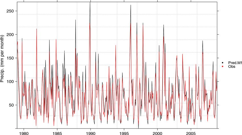
Figure 1. Schematic overview of the R package downscaleR and its framing into the climate4R framework for climate data access and
analysis. The typical perfect-prognosis downscaling phases are indicated by the gray arrows. (i) In the first place, model setup is undertaken.
This process is iterative and usually requires testing many different model configurations under a cross-validation setup until an optimal
configuration is achieved. The downscaleCV function (and prepareData under the hood) is used in this stage for a fine-tuning of the
model. Model selection is determined through the use of indices and measures reflecting model suitability for different aspects that usually
depend on specific research aims (e.g., good reproducibility of extreme events, temporal variability, spatial dependency across different
locations). The validation is achieved through the climate4R.value package (red-shaded callout), implementing the VALUE validation
framework. (ii) Model training: once an optimal model is achieved, model training is performed using the downscaleTrain function.
(iii) Finally, the calibrated model is used to undertake downscaling (i.e., model predictions) using the function downscalePredict.
The data to be used in the predictions requires appropriate preprocessing (e.g., centering and scaling using the predictor set as reference,
projection of PCs onto predictor EOFs) that is performed under the hood by the function prepareNewData prior to model prediction with
downscalePredict.
already shown in Iturbide et al. (2019). Here, the focus is on midity, geopotential, or air temperature (see Sect. 3.1.2) at
the implementation of PP methods that entail greater techni- different surface pressure vertical levels. Only sea-level pres-
cal complexities for their application from a user’s perspec- sure and 2 m air temperature are usually used as near-surface
tive but have received less attention from the side of climate predictors. An example of the evaluation of this hypothesis is
service development. A schematic diagram showing the main later presented in Sect. 4.2.1 of this study. Often, predictors
phases of perfect-prognosis downscaling is shown in Fig. 1. are proxies for physical processes, which is a main reason for
non-stationarities in the predictor–predictand relationship, as
2.1 SDS model setup: configuration of predictors amply discussed in Maraun and Widmann (2018). Further-
more, reanalysis choice has been reported as an additional
As general recommendations, a number of aspects need to source of uncertainty for SDS model development (Brands
be carefully addressed when looking for suitable predictors et al., 2012), although its effect is of relevance only in the
in the PP approach (Wilby et al., 2004; Hanssen-Bauer et al., tropics (see, e.g., Manzanas et al., 2015). With regard to
2005): (i) the predictors should account for a major part of the assumption (ii), predictor selection and the training of
the variability in the predictands, (ii) the links between pre- transfer functions are carried out on short-term variability
dictors and predictands should be temporally stable or sta- in present climate, whereas the aim is typically to simulate
tionary, and (iii) the large-scale predictors must be realisti- long-term changes in short-term variability (Huth, 2004; Ma-
cally reproduced by the global climate model. Since differ- raun and Widmann, 2018), which limits the performance of
ent global models are used in the calibration and downscaling PP and makes it particularly sensitive to the method type and
phases, large-scale circulation variables well represented by the predictor choice (Maraun et al., 2019b).
the global models are typically chosen as predictors in the For all these reasons, the selection of informative and ro-
PP approach, whereas variables directly influenced by model bust predictors during the calibration stage is a crucial step
parametrizations and/or orography (e.g., precipitation) are in SDS modeling (Fig. 1), model predictions being very sen-
usually not considered. For instance, predictors generally ful- sitive to the strategy used for predictor configuration (see,
filling these conditions for downscaling precipitation are hu-
Geosci. Model Dev., 13, 1711–1735, 2020 www.geosci-model-dev.net/13/1711/2020/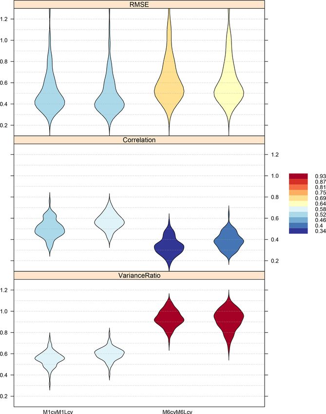
J. Bedia et al.: Statistical downscaling with downscaleR                                                                     1715

e.g., Benestad, 2007; Gutiérrez et al., 2013). PP techniques              other global predictors (either raw fields – case 1 – or
can consider point-wise and/or spatial-wise predictors, using             principal components – case 2) encompassing a larger
either the raw values of a variable over a region of a user-              spatial domain.
defined extent or only at nearby grid boxes and/or the prin-
cipal components (PCs) corresponding to the empirical or-            Therefore, predictor screening (i.e., variable selection) and
thogonal functions (EOFs; Preisendorfer, 1988) of the vari-       their configuration is one of the most time-consuming tasks
ables considered over a representative geographical domain        in perfect-prognosis experiments due to the potentially huge
(which must be also conveniently determined). Usually, the        number of options required for a fine-tuning of the predic-
latter are more informative in those cases where the local cli-   tor set (spatial, local, or a combination of both, number of
mate is mostly determined by synoptic phenomena, whereas          principal components, and methodology for their genera-
the former may be needed to add some information about the        tion, etc.). As a result, SDS model tuning is iterative and
local variability in those cases where small-scale processes      usually requires testing many different model configurations
are important (see, e.g., Benestad, 2001). Sometimes, both        until an optimal one is attained (see, e.g., Gutiérrez et al.,
types of predictors are combined in order to account for both     2013), as next described in Sect. 2.3. This requires a flexi-
synoptic and local effects. In this sense, three non-mutually     ble yet easily configurable interface, enabling users to launch
exclusive options are typically used in the downscaling ex-       complex experiments for testing different predictor setups
periments next summarized:                                        in a straightforward manner. In downscaleR, the function
                                                                  prepareData has been designed to this aim, providing
 1. using raw atmospheric fields for a given spatial domain,      maximum user flexibility for the definition of all types of
    typically continental- or nation-wide for downscaling         predictor configurations with a single command call, build-
    monthly and daily data, respectively. For instance, in        ing upon the raw predictor information (see Sect. 3.3).
    the VALUE experiment, predefined subregions within
    Europe are used for training (Fig. 2), thus helping to re-    2.2     Description of SDS methods
    duce the dimension of the predictor set. Alternatively,
    stepwise or regularized methods can be used to auto-          downscaleR implements several PP techniques, ranging
    matically select the predictor set from the full spatial      from the classical analogs and regression to more recent
    domain.                                                       and sophisticated machine-learning methods (Baño-Medina
                                                                  et al., 2019). For brevity, in this study we focus on the stan-
 2. using principal components obtained from these fields         dard approaches contributing to the VALUE intercompari-
    (Benestad, 2001). Working with PCs allows users to            son, namely analogs, linear models, and generalized linear
    filter out high-frequency variability which may not be        models, next briefly introduced; the up-to-date description
    properly linked to the local scale, greatly reducing the      of methods is available at the downscaleR wiki (https:
    dimensionality of the problem related to the deletion         //github.com/SantanderMetGroup/downscaleR/wiki, last ac-
    of redundant and/or collinear information from the raw        cess: 29 March 2020). All the SDS methods im-
    predictors. These predictors convey large-scale infor-        plemented in downscaleR are applied using unique
    mation to the predictor set and are often also referred to    workhorse functions, such as downscaleCV (cross-
    as “spatial predictors”. These can be a number of prin-       validation), downscaleTrain (for model training), and
    cipal components calculated upon each particular vari-        downscalePredict (for model prediction) (Fig. 1), that
    able (e.g., explaining 95 % of the variability) and/or a      receive the different tuning parameters for each method cho-
    combined PC calculated upon the (joined) standardized         sen, providing maximum user flexibility for the definition
    predictor fields (“combined” PCs).                            and calibration of the methods. Their application will be il-
                                                                  lustrated throughout Sects. 3.3 and 4.
 3. The spatial extent of each predictor field may have a
    strong effect on the resulting model. Some variables          2.2.1     Analogs
    of the predictor set may have explanatory power only
    nearby the predictand locations, while the useful infor-      This is a non-parametric analog technique (Lorenz, 1969;
    mation is diluted when considering larger spatial do-         Zorita and von Storch, 1999), based on the assumption that
    mains. As a result, it is common practice to include local    similar (or analog) atmospheric patterns (predictors) over a
    information in the predictor set by considering only a        given region lead to similar local meteorological outcomes
    few grid points around the predictand location for some       (predictand). For a given atmospheric pattern, the corre-
    of the predictor variables (this can be just the closest      sponding local prediction is estimated according to a de-
    grid point or a window of a user-defined width). This         termined similarity measure (typically the Euclidean norm,
    category can be regarded as a particular case of point        which has been shown to perform satisfactorily in most
    1 but considering a much narrower window centered             cases; see, e.g., Matulla et al., 2008) from a set of analog pat-
    around the predictand location. This local information        terns within a historical catalog over a representative clima-
    is combined with the “global” information provided by         tological period. In PP, this catalog is formed by reanalysis

www.geosci-model-dev.net/13/1711/2020/                                                Geosci. Model Dev., 13, 1711–1735, 2020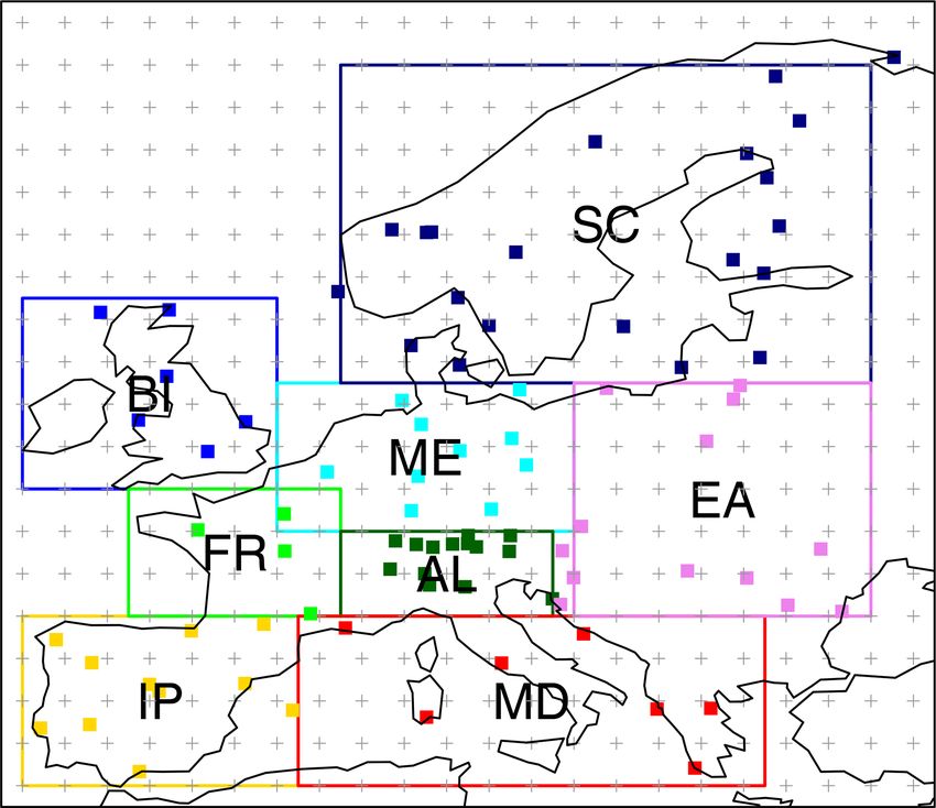
1716                                                                 J. Bedia et al.: Statistical downscaling with downscaleR

data. In spite of its simplicity, analog performance is com-        is used to downscale precipitation occurrence (0 = no rain;
petitive against other more sophisticated techniques (Zorita        1 = rain) and a GLM with gamma error distribution and log
and von Storch, 1999), being able to take into account the          canonical link function is used to downscale precipitation
non-linearity of the relationships between predictors and pre-      amount, considering wet days only. After model calibration,
dictands. Additionally, it is spatially coherent by construc-       new daily predictions are given by simulating from a gamma
tion, preserving the spatial covariance structure of the lo-        distribution, whose shape parameter is fitted using the ob-
cal predictands as long as the same sequence of analogs for         served wet days in the calibration period.
different locations is used, spatial coherence being underes-          Beyond the classical GLM configurations, downscaleR
timated otherwise (Widmann et al., 2019). Hence, analog-            allows using both deterministic and stochastic versions of
based methods have been applied in several studies both             GLMs. In the former, the predictions are obtained from the
in the context of climate change (see, e.g., Gutiérrez et al.,      expected values estimated by both the GLM for occurrence
2013) and seasonal forecasting (Manzanas et al., 2017). The         (GLMo) and the GLM for amount (GLMa). In the GLMo,
main drawback of the analog technique is that it cannot pre-        the continuous expected values ∈ [0, 1] are transformed into
dict values outside the observed range, therefore being par-        binary ones as 1 (0) either by fixing a cutoff probability value
ticularly sensitive to the non-stationarities arising in climate    (e.g., 0.5) or by choosing a threshold based on the observed
change conditions (Benestad, 2010) and thus preventing its          predictand climatology for the calibration period (the latter
application to the far future, when temperature and directly        is the default behavior in downscaleR). By contrast, for
related variables are considered (see, e.g., Bedia et al., 2013).   GLMa, the expected values are directly interpreted as rain
                                                                    amounts. Moreover, downscaleR gives the option of gen-
2.2.2   Linear models (LMs)                                         erating stochastic predictions for both the GLMo the and
                                                                    GLMa, which could be seen as a dynamic predictor-driven
(Multiple) linear regression is the most popular downscaling        version of the inflation of variance used in some regression-
technique for suitable variables (e.g., temperature), although      based methods (Huth, 1999).
it has been also applied to other variables after suitable trans-
formation (e.g., to precipitation, typically taking the cubic       2.3   SDS model validation
root). Several implementations have been proposed includ-
ing spatial (PC) and/or local predictors. Moreover, automatic       When assessing the performance of any SDS technique it
predictor selection approaches (e.g., stepwise) have been also      is crucial to properly cross-validate the results in order to
applied (see Gutiérrez et al., 2019, for a review).                 avoid misleading conclusions about model performance due
                                                                    to artificial skill. This is typically achieved considering a
2.2.3   Generalized linear models (GLMs)
                                                                    historical period for which observations exist to validate
They were formulated by Nelder and Wedderburn (1972) in             against. k-fold and leave-one-out cross-validation are among
the 1970s and are an extension of the classical linear re-          the most widely applied validation procedures in SDS ex-
gression, which allows users to model the expected value of         periments. In a k-fold cross-validation framework (Stone,
a random predictand variable whose distribution belongs to          1974; Markatou et al., 2005), the original sample (histor-
the exponential family (Y ) through an arbitrary mathemati-         ical period) is partitioned into k equally sized and mutu-
cal function called link function (g) and a set of unknown          ally exclusive subsamples (folds). In each of the k iterations,
parameters (β), according to                                        one of these folds is retained for testing (prediction phase)
                                                                    and the remaining k − 1 folds are used for training (calibra-
E(Y ) = µ = g −1 (Xβ),                                       (1)    tion phase). The resulting k independent samples are then
                                                                    merged to produce a single time series covering the whole
where X is the predictor and E(Y ) the expected value of the        calibration period, which is subsequently validated against
predictand. The unknown parameters, β, can be estimated             observations. When k = n (being n the number of observa-
by maximum likelihood, considering a least-squares iterative        tions), the k-fold cross-validation is exactly the leave-one-
algorithm.                                                          out cross-validation (Lachenbruch and Mickey, 1968). An-
   GLMs have been extensively used for SDS in climate               other common approach is the simpler “holdout” method,
change applications (e.g., Brandsma and Buishand, 1997;             that partitions the data into just two mutually exclusive sub-
Chandler and Wheater, 2002; Abaurrea and Asín, 2005;                sets (k = 2), called the training and test (or holdout) sets. In
Fealy and Sweeney, 2007; Hertig et al., 2013) and, more re-         this case, it is common to designate two-thirds of the data
cently, also for seasonal forecasts (Manzanas et al., 2017).        as the training set and the remaining one-third as the test set
For the case of precipitation, a two-stage implementation           (see, e.g., Kohavi, 1995).
(see, e.g., Chandler and Wheater, 2002) must be used given             Therefore, PP models are first cross-validated under “per-
its dual (occurrence–amount) character. In this implemen-           fect conditions” (i.e., using reanalysis predictors) in order
tation, a GLM with Bernoulli error distribution and logit           to evaluate their performance against real historical climate
canonical link function (also known as logistic regression)         records before being applied to “non-perfect” GCM pre-

Geosci. Model Dev., 13, 1711–1735, 2020                                               www.geosci-model-dev.net/13/1711/2020/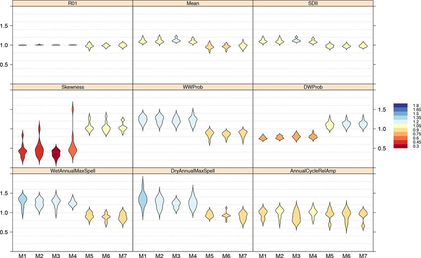
J. Bedia et al.: Statistical downscaling with downscaleR                                                                       1717

dictors. Therefore, the aim of cross-validation in the PP
approach is to properly estimate, given a known predictor
dataset (large-scale variables from reanalysis), the perfor-
mance of the particular technique considered, having an “up-
per bound” for its generalization capability when applied to
new predictor data (large-scale variables from GCM). The
workhorse for cross-validation in downscaleR is the func-
tion downscaleCV, which adequately handles data parti-
tion to create the training and test data subsets according to
the parameters specified by the user, being tailored to the spe-
cial needs of statistical downscaling experiments (i.e., ran-
dom temporal or spatial folds, leave-one-year-out, arbitrary
selection of years as folds, etc.).
   During the cross-validation process, one or several user-
defined measures are used in order to assess model perfor-
mance (i.e., to evaluate how “well” do model predictions
match the observations), such as accuracy measures, distri-
butional similarity scores, inter-annual variability, and trend
matching scores. In this sense, model quality evaluation is        Figure 2. Location of the 86 stations of the ECA-VALUE-86
a multi-faceted task with many possible and often unrelated        dataset (red squares). The colored boxes show the eight PRU-
aspects to look into. Thus, validation ultimately consists of      DENCE subregions considered in the VALUE downscaling exper-
deriving specific climate indices from model output, com-          iment for model training (Sect. 3.1). The regular grid of the pre-
paring these indices to reference indices calculated from ob-      dictor dataset, a 2◦ ×2◦ resolution version of the ERA-Interim re-
servational data and quantifying the mismatch with the help        analysis, is also shown. The subregions considered are IP (Iberian
of suitable performance measures (Maraun et al., 2015). In         Peninsula), FR (France), BI (British Isles), MD (Mediterranean),
VALUE, the term “index” is used in a general way, in-              AL (Alps), ME (central Europe), SC (Scandinavia), and EA (east-
cluding not only single numbers (e.g., the 90th percentile         ern Europe). Station metadata can be interactively queried through
of precipitation, lag-1 autocorrelation) but also vectors such     the VALUE Validation Portal application (http://www.value-cost.
                                                                   eu/validationportal/app/#!datasets, last access: 29 March 2020).
as time series (for instance, a binary time series of rain or
no rain). Specific “measures” are then computed upon the
predicted and observed indices, for instance the difference
(bias, predicted – observed) of numeric indices or the corre-      3   Illustrative case study: the VALUE experiment
lation of time series (Sect. 3.3.9). A comprehensive list of
indices and measures has been elaborated by the VALUE              The VALUE initiative (Maraun et al., 2015) produced the
cross-cutting group in order to undertake a systematic evalu-      largest-to-date intercomparison of statistical downscaling
ation of downscaling methods. The complete list is presented       methods with over 50 contributing techniques. The contribu-
in the VALUE Validation Portal (http://www.value-cost.eu/          tion of MeteoLab (and downscaleR) to this experiment
validationportal/app/#!indices, last access: 29 March 2020).       included a number of methods which are fully reproducible
Furthermore, all the VALUE indices and measures have               with downscaleR, as we show in this example. This pan-
been implemented in R and collected in the package VALUE           European contribution was based on previous experience
(https://github.com/SantanderMetGroup/VALUE, last ac-              over the Iberian domain (Gutiérrez et al., 2013; San-Martín
cess: 29 March 2020), allowing for further collabora-              et al., 2016), testing a number of predictor combinations and
tion and extension with other initiatives, as well as              method configurations. In order to illustrate the application
for research reproducibility. The validation tools avail-          of downscaleR, in this example we first revisit the ex-
able in VALUE have been adapted to the specific data               periment over Iberian domain (but considering the VALUE
structures of the climate4R framework (see Sect. 1)                framework and data), showing the code undertaking the dif-
through the wrapping package climate4R.value (https:               ferent steps (Sect. 3.3). Afterwards, the subset of methods
//github.com/SantanderMetGroup/climate4R.value, last ac-           contributing to VALUE is applied at a pan-European scale,
cess: 29 March 2020), enabling a direct application of the         including also results of future climate scenarios (Sect. 4).
comprehensive VALUE validation framework to downscal-                 In order to reproduce the results of the VALUE inter-
ing exercises with downscaleR (Fig. 1). A summary of the           comparison, the VALUE datasets are used in this study
subset of VALUE indices and measures used in this study is         (Sect. 3.1). In addition, future projections from a CMIP5
presented in Table 1.                                              GCM are also used to illustrate the application of the down-
                                                                   scaling methods to climate change studies. For transparency
                                                                   and full reproducibility, the datasets are public and freely

www.geosci-model-dev.net/13/1711/2020/                                                Geosci. Model Dev., 13, 1711–1735, 2020
1718                                                                                     J. Bedia et al.: Statistical downscaling with downscaleR

Table 1. Summary of the subset of VALUE validation indices and measures used in this study. Their codes are consistent with the VALUE
reference list (http://www.value-cost.eu/validationportal/app/#!indices), except for “ts.ks.pval”, which has been included later in the VALUE
set of measures.

                       Code                            Description                                                               Type
                       R01                             Relative frequency of wet days (precip ≥ 1 mm)                            Index
                       Mean                            Mean                                                                      Index
                       SDII                            Simple daily intensity index                                              Index
                       Skewness                        Skewness                                                                  Index
                       WWProb                          Wet–wet transition probability (wet ≥ 1 mm)                               Index
                       DWProb                          Dry–wet transition probability (wet ≥ 1 mm)                               Index
                       WetAnnualMaxSpell               Median of the annual wet (≥ 1 mm) spell maxima                            Index
                       DryAnnualMaxSpell               Median of the annual dry (< 1 mm) spell maxima                            Index
                       AnnualCycleAmp                  Amplitude of the daily annual cycle                                       Index
                       Var                             Quasi-variance                                                            Index
                       ratio                           Ratio predicted/observed                                                  Measure1
                       ts.rs                           Spearman correlation                                                      Measure2
                       ts.RMSE                         Root mean square error                                                    Measure2
                       ts.ks                           Two-sample Kolmogorov–Smirnov (KS) test statistic                         Measure2,3
                       ts.ks.pval                      (corrected) p value of the two sample KS test statistic                   Measure2,3
                     The superscripts in the measures indicate the input used to compute them: 1 – a single scalar value, corresponding to the
                     predicted and observed indices; 2 – the original predicted and observed precipitation time series; 3 – transformed time series
                     (centered anomalies or standardized anomalies).

available for download using the climate4R tools, as                                   3.1.2      Predictor data (reanalysis)
indicated in Sect. 3.2. Next, the datasets are briefly pre-
sented. Further information on the VALUE data character-                               In line with the experimental protocol of the Coordinated Re-
istics is given in Maraun et al. (2015) and Gutiérrez et al.                           gional Climate Downscaling Experiment (CORDEX; Giorgi
(2019) and also at their official download URL (http://www.                            et al., 2009), VALUE has used ERA-Interim (Dee et al.,
value-cost.eu/data, last access: 29 March 2020). The refer-                            2011) as the reference reanalysis to drive the experiment with
ence period considered for model evaluation in perfect con-                            perfect predictors. For full comparability, the list of predic-
ditions is 1979–2008. In the analysis of the GCM predic-                               tors used in VALUE is replicated in this study – see Table 2
tors (Sect. 4.2.1), this period is adjusted to 1979–2005 con-                          in Gutiérrez et al. (2019) – namely sea-level pressure, 2 m
strained by the period of the historical experiment of the                             air temperature, air temperature and relative humidity at 500,
CMIP5 models (Sect. 3.1.3). The future period for presenting                           700, and 850 hPa surface pressure levels, and the geopoten-
the climate change signal analysis is 2071–2100.                                       tial height at 500 hPa.
                                                                                          The set of raw predictors corresponds to the full European
3.1     Datasets                                                                       domain shown in Fig. 2. The eight reference regions defined
                                                                                       in the PRUDENCE project of model evaluation (Christensen
3.1.1    Predictand data (weather station records)
                                                                                       et al., 2007) were used in VALUE as appropriate regional do-
The European station dataset used in VALUE has been care-                              mains for training the models of the corresponding stations
fully prepared in order to be representative of the different                          (Sect. 2.1). The stations falling within each domain are col-
European climates and regions and with a reasonably ho-                                ored accordingly in Fig. 2.
mogeneous spatial density (Fig. 2). To keep the exercise as
open as possible, the downloadable (blended) ECA&D sta-                                3.1.3      Predictor data (GCM future projections)
tions (Klein Tank et al., 2002) were used. From this, a final
subset of 86 stations was selected with the help of local ex-                          In order to illustrate the application of SDS methods to down-
perts in the different countries, restricted to high-quality sta-                      scale future global projections from GCM predictors, here
tions with no more than 5 % of missing values in the analysis                          we consider the outputs from the EC-EARTH model (in par-
period (1979–2008). Further details on predictand data pre-                            ticular the r12i1p1 ensemble member; EC-Earth Consortium,
processing are provided in http://www.value-cost.eu/WG2_                               2014) for the 2071–2100 period under the RCP8.5 scenario
dailystations (last access: 29 March 2020). The full list of                           (Moss et al., 2010). This simulation is part of CMIP5 (Tay-
stations is provided in Table 1 in Gutiérrez et al. (2019).                            lor et al., 2011) and is officially served by the Earth System
                                                                                       Grid Federation infrastructure (ESGF; Cinquini et al., 2014).
                                                                                       In this study, data are retrieved from the Santander User Data

Geosci. Model Dev., 13, 1711–1735, 2020                                                                         www.geosci-model-dev.net/13/1711/2020/
J. Bedia et al.: Statistical downscaling with downscaleR 1719 Gateway (Sect. 4.2), which is the data access layer of the vars
1720                                                                       J. Bedia et al.: Statistical downscaling with downscaleR

Table 2. Summary of predictor configurations tested. Local predictors always correspond to the original predictor fields previously stan-
dardized. Independent PCs are calculated separately for each predictor field, while combined PCs are computed upon the previously joined
predictor fields (see Sect. 2.1 for more details). a The standardization in M5 is performed by subtracting to each grid cell the overall field
mean, so the spatial structure of the predictor is preserved. Methods marked with b are included in the VALUE intercomparison, with the
slight difference that in VALUE, a fixed number of 15 PCs is used and here the number varies slightly until achieving the percentage of
explained variance indicated (in any case, the differences are negligible in terms of model performance). Methods followed by the -L suffix
(standing for “local”) are used only in the pan-European experiment described in Sect. 4.

                Method     ID            Predictor configuration description
                           arguments
                           M1b           Spatial: n combined PCs explaining 95 % of variance
                           M1-L          Spatial+local: n combined PCs explaining 95 % of variance + first nearest grid box
                GLM        M2            Spatial: n independent PCs explaining 95 % of the variance
                           M3            Local: first nearest grid box
                           M4            Local: four nearest grid boxes
                           M5            Spatial: original standardizeda predictor fields
                           M6b           Spatial: n combined PCs explaining 95 % of variance
                Analogs
                           M6-L          Local: 25 nearest grid boxes
                           M7            Spatial: n independent PCs explaining 95 % of the variance

y
J. Bedia et al.: Statistical downscaling with downscaleR 1721
point). As the optimal predictor configuration is chosen af- family = binomial(link = "logit"),
ter cross-validation, typically the function downscaleCV folds = folds,
is used in first place. The latter function makes internal calls prepareData.args = list(global.vars =
to prepareData recursively for the different training sub-
sets defined. NULL,
local.predictors =
As a result, downscaleCV receives as input all the ar-
NULL,
guments of prepareData for predictor configuration as spatial.predictors =
a list, plus other specific arguments controlling the cross- spatial.pars.M1,
validation setup. For instance, the argument folds allows combined.only = TRUE))
specifying the number of training or test subsets to split the
In the logistic regression model, downscaleCV returns
dataset in. In order to perform the classical leave-one-year-
a multigrid with two output prediction grids, storing the vari-
out cross-validation schema, folds should equal the total ables prob and bin. The first contains the grid probability of
number of years encompassing the full training period (e.g., rain for every day and the second is a binary prediction indi-
folds=list(1979:2008)). The way the different sub- cating whether it rained or not. Thus, in this case the binary
samples are split is controlled by the argument type, provid- output is retained, using subsetGrid along the “var” di-
ing fine control on how the random sampling is performed. mension:
Here, in order to replicate the VALUE experimental frame-
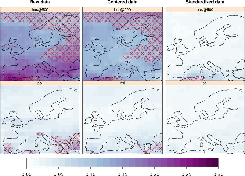
M1cv.bin1722 J. Bedia et al.: Statistical downscaling with downscaleR Figure 3. Cross-validated predictions of monthly accumulated precipitation by the method M1 (black), plotted against the corresponding observations (red). Both time series have been spatially aggregated considering the 11 stations within the Iberian subdomain. 3.3.3 Configuration of method M2 scaling.pars
J. Bedia et al.: Statistical downscaling with downscaleR                                                                       1723

of the standardized field. To account for this particularity, the
scaling parameters are modified accordingly, via the argu-
ment spatial.frame = "field", which is internally
passed to scaleGrid.
scaling.pars.M5
1724                                                                J. Bedia et al.: Statistical downscaling with downscaleR

data availability” section). Violins are in essence a combina-     loadGridData function. These arguments can be omitted
tion of a box plot and a kernel density plot. Box plots are        in the case of the station data load, since all the available sta-
a standard tool for inspecting the distribution of data most       tions are requested in this case. The full code used in this step
users are familiar with, but they lack basic information when      is detailed in the notebook accompanying this paper (see the
data are not normally distributed. Density plots are more use-     “Code and data availability” section).
ful when it comes to comparing how different datasets are
distributed. For this reason, violin plots incorporate the in-     4.1   Method intercomparison experiment
formation of kernel density plots in a box-plot-like represen-
tation and are particularly useful to detect bimodalities or de-   The configuration of predictors is indicated through the pa-
partures from the normal distribution of the data, intuitively     rameter lists, as shown throughout Sects. 3.3.2 to 3.3.8. In
depicted by the shape of the violins. The violins are inter-       the case of method M1-L, local predictors considering the
                                                                   first nearest grid box are included in the M1 configuration
nally produced by the package lattice (Sarkar, 2008) via
                                                                   (Table 2):
the panel function panel.violin to which the interested
reader is referred for further details on violin plot design and   M1.L
J. Bedia et al.: Statistical downscaling with downscaleR 1725
Figure 5. Cross-validation results obtained by the seven methods tested (M1 to M7, Table 2) according to the core set of validation indices
defined in the VALUE intercomparison experiment, considering the subset of the Iberian Peninsula stations (n = 11). The color bar indicates
the mean ratio (predicted/observed) measure calculated for each validation index (Table 1).
Table 3. Validation results of the four methods tested in the pan-European experiment. The values presented (from left to right: minimum,
first quartile, median, third quartile, maximum, and standard deviation) correspond to the violin plots displayed in Fig. 6 (n = 86 stations).
Note that, for consistency with Fig. 6, the RMSE results are multiplied by a factor of 0.1 in order to attain a similar order of magnitude for
the three validation measures considered. This is also indicated in the caption of Fig. 6.
Min. First qu. Median Mean Third qu. Max. SD
RMSE(×0.1)
M1cv 0.27 0.39 0.45 0.52 0.60 1.41 0.20
M1Lcv 0.25 0.37 0.43 0.49 0.58 1.33 0.19
M6cv 0.33 0.49 0.57 0.67 0.78 1.96 0.28
M6Lcv 0.32 0.47 0.55 0.64 0.74 1.74 0.26
Correlation
M1cv 0.32 0.45 0.50 0.50 0.55 0.76 0.09
M1Lcv 0.40 0.52 0.56 0.57 0.62 0.76 0.07
M6cv 0.16 0.28 0.34 0.34 0.39 0.56 0.08
M6Lcv 0.25 0.33 0.39 0.39 0.44 0.63 0.08
Variance ratio
M1cv 0.32 0.52 0.55 0.55 0.59 0.74 0.07
M1Lcv 0.41 0.57 0.60 0.60 0.63 0.79 0.06
M6cv 0.72 0.88 0.93 0.93 0.99 1.08 0.08
M6Lcv 0.64 0.86 0.94 0.92 0.98 1.10 0.10
4.2 Future downscaled projections regarding the good representation by the GCM of the reanal-
ysis predictors is assessed in Sect. 4.2.1.
In this section, the calibrated SDS models are used to down-
scale GCM future climate projections from the CMIP5 EC-
EARTH model (Sect. 3.1.3). Before generating the model
predictions (Sect. 4.2.2), the perfect-prognosis assumption
www.geosci-model-dev.net/13/1711/2020/ Geosci. Model Dev., 13, 1711–1735, 20201726 J. Bedia et al.: Statistical downscaling with downscaleR
series on a grid box basis, considering the original continuous
daily time series for their common period, 1979–2005. In or-
der to isolate distributional dissimilarities due to errors in the
first- and second-order moments, we also consider anoma-
lies and standardized anomalies (the latter being used as ac-
tual predictors in the SDS models). The anomalies are cal-
culated by removing the overall grid box mean to each daily
value, and in the case of the standardized anomalies, we ad-
ditionally divide by the seasonal standard deviation. Due to
the strong serial correlation present in the daily time series,
the test is prone to inflation of type-1 error, that is, rejecting
the null hypothesis of equal distributions when it is actually
true. To this aim, an effective sample size correction has been
applied to the data series to calculate the p values (Wilks,
2006). The methodology follows the procedure described in
Brands et al. (2012, 2013), implemented by the VALUE mea-
sure “ts.ks.pval” (Table 1).
The distributions of GCM and reanalysis (Fig. 7) differ
significantly when considering the raw time series, thus vi-
olating the assumptions of the PP hypothesis. Centering the
data (i.e, zero mean time series) greatly alleviates this prob-
lem for most variables, excepting specific humidity at 500 mb
(“hus@500”) and near-surface temperature (tas; not shown
here, but displayed in the paper notebook). Finally, data
standardization improves the distributional similarity, attain-
ing an optimal representation of all the GCM predictors but
hus@500 over a few grid points in the Mediterranean.
Figure 6. Cross-validation results obtained by the four methods
The distributional similarity analysis is straightforward us-
tested (M1, M1-L, M6, and M6-L; Table 2) in the pan-European
ing the functions available in climate4R, already shown in
experiment (n = 86 stations), according to three selected validation
measures (Spearman correlation, RMSE, and variance ratio; see Ta- the previous examples. For brevity, the code generating Fig. 7
ble 1). The color bar indicates the mean value of each measure. A is omitted here, and included with extended details and for
factor of 0.1 has been applied to the RMSE in order to attain the all the predictor variables in the notebook accompanying this
same order of magnitude in the y axis for all the validation mea- paper (see the “Code and data availability” section).
sures.
– Data centering or standardization is performed di-
rectly using the function scaleGrid and using the
4.2.1 Assessing the GCM representation of the appropriate argument values type="center" or
predictors "standardize", respectively.
As indicated in Sect. 2.1, PP model predictions are built un- – The KS test is directly launched using the
der the assumption that the GCM is able to adequately re- function valueMeasure from the package
produce the predictors taken from the reanalysis. Here, this climate4R.VALUE and including the argu-
question is addressed through the evaluation of the distri- ment value measure.code="ts.ks" and
butional similarity between the predictor variables, as rep- "ts.ks.pval" for KS score and its (corrected)
resented by the EC-EARTH model in the historical simula- p value, respectively.
tion, and the ERA-Interim reanalysis. To this aim, the two-
sample Kolmogorov–Smirnov test is used, included in the – The KS score maps and the stippling based on their p
set of validation measures of the VALUE framework and values are produced with the function spatialPlot
thus implemented in the VALUE package. The KS test is from package visualizeR.
a non-parametric statistical hypothesis test for checking the
null hypothesis (H0 ) that two candidate datasets come from In conclusion, although not all predictors are equally well
the same underlying theoretical distribution. The statistic is represented by the GCM, data standardization is able to solve
bounded between 0 and 1, indicating that the lower values the problem of distributional dissimilarities, even in the case
have a greater distributional similarity. The KS test is first of the worst represented variable, that is, specific humidity at
applied to the EC-EARTH and ERA-Interim reanalysis time 500 mb level.
Geosci. Model Dev., 13, 1711–1735, 2020 www.geosci-model-dev.net/13/1711/2020/J. Bedia et al.: Statistical downscaling with downscaleR 1727
Figure 7. KS score maps, depicting the results of the two-sample KS test applied to the time series from the EC-EARTH GCM and ERA-
Interim, considering the complete time series for the period 1979–2005. The results are displayed for two of the predictor variables (by rows),
namely specific humidity at 500 mb surface pressure height (“hus@500”, badly represented by the GCM) and mean sea-level pressure (“psl”,
well represented by the GCM). The KS test results are displayed by columns, using, from left to right, the raw, the zero-mean (centered),
and the zero-mean and unit variance (standardized) time series from both the reanalysis and the GCM. The grid boxes showing low p values
(p < 0.05) have been marked with a red cross, indicating significant differences in the distribution of both GCM and reanalysis time series.
4.2.2 Future SDS model predictions After SDS model calibration downscalePredict is
the workhorse for downscaling. First of all, the GCM
The final configuration of predictors for M1-L (stored in the datasets required are obtained. As previously done with
M1.L list) and M6-L methods (M6.L) is directly passed ERA-Interim, the EC-EARTH simulations are obtained from
the climate4R UDG, considering the same set of variables
to the function prepareData, whose output contains all
already used for training the models (Sect. 3.1.2). Again, the
the information required to undertake model training via the individual predictor fields are recursively loaded and stored
downscaleTrain function. In the following, the code for in a climate4R multigrid.
the analog method is presented. Note that for GLMs the code
is similar but taking into account occurrence and amount in historical.datasetYou can also read