Revised planet brightness temperatures using the Planck/LFI 2018
←
→
Page content transcription
If your browser does not render page correctly, please read the page content below
Astronomy & Astrophysics manuscript no. aa_2020_37788_maris_et_al_v2                                                                  ©ESO 2021
                                               March 17, 2021

                                               Revised planet brightness temperatures using the Planck/LFI 2018
                                                                        data release?
                                                Michele Maris1?? , Erik Romelli1 , Maurizio Tomasi2 , Anna Gregorio3, 1 , Maura Sandri4 , Samuele Galeotta1 , Daniele
                                                                     Tavagnacco1 , Marco Frailis1 , Gianmarco Maggio1 , and Andrea Zacchei1

                                                     1
                                                         INAF/Trieste Astronomical Observatory, Via G.B.Tiepolo 11 - 34143, Trieste, Italy
                                                     2
                                                         Dipartimento di Fisica ”Aldo Pontremoli”, Università degli Studi di Milano, Via G.Celoria 16, 20133, Milano, Italy
                                                     3
                                                         Trieste University: Physics Department, Via A. Valerio 2 - 34127, Trieste, Italy
                                                     4
                                                         INAF/Bologna Astronomical Observatory, Via Gobetti 93/3 - 40129, Bologna, Italy
arXiv:2012.04504v2 [astro-ph.EP] 16 Mar 2021

                                                     March 16, 2021

                                                    DOI: 10.1051/0004-6361/202037788;
                                                    arxiv: 2012.04504;
                                                    Journal: A&A, 2021, 647, A104

                                                    Versioning:
                                                     V2     March 16, 2021       as published on the journal
                                                                                                                                     l
                                                     V1     December 9, 2021     as accepted for the pubblication on A&A Dec 3, 2020

                                                                                                                   ABSTRACT

                                                    Aims. We present new estimates of the brightness temperatures of Jupiter, Saturn, Uranus, and Neptune based on the measurements
                                                    carried in 2009–2013 by Planck/LFI at 30, 44, and 70 GHz and released to the public in 2018. This work extends the results presented
                                                    in the 2013 and 2015 Planck/LFI Calibration Papers, based on the data acquired in 2009–2011.
                                                    Methods. Planck observed each planet up to eight times during the nominal mission. We processed time-ordered data from the 22 LFI
                                                    radiometers to derive planet antenna temperatures for each planet and transit. We accounted for the beam shape, radiometer bandpasses,
                                                    and several systematic effects. We compared our results with the results from the ninth year of WMAP, Planck/HFI observations, and
                                                    existing data and models for planetary microwave emissivity.
                                                    Results. For Jupiter, we obtain T b = 144.9, 159.8, 170.5 K (±0.2 K at 1σ, with temperatures expressed using the Rayleigh-Jeans
                                                    scale) at 30, 44 and 70 GHz, respectively, or equivalently a band averaged Planck temperature T b(ba) = 144.7, 160.3, 171.2 K in good
                                                    agreement with WMAP and existing models. A slight excess at 30 GHz with respect to models is interpreted as an effect of synchrotron
                                                    emission. Our measures for Saturn agree with the results from WMAP for rings T b = 9.2 ± 1.4, 12.6 ± 2.3, 16.2 ± 0.8 K, while for the
                                                    disc we obtain T b = 140.0 ± 1.4, 147.2 ± 1.2, 150.2 ± 0.4 K, or equivalently a T b(ba) = 139.7, 147.8, 151.0 K. Our measures for Uranus
                                                    (T b = 152 ± 6, 145 ± 3, 132.0 ± 2 K, or T b(ba) = 152, 145, 133 K) and Neptune (T b = 154 ± 11, 148 ± 9, 128 ± 3 K, or T b(ba) = 154, 149,
                                                    128 K) agree closely with WMAP and previous data in literature.
                                                    Key words. Cosmology: cosmic background radiation - Planets and satellites: general - Instrumentation: detectors - Methods: data
                                                    analysis

                                               1. Introduction                                                      the High Frequency Instrument (HFI) was an array of bolometers
                                                                                                                    working in the 100–850 GHz range, while the Low Frequency
                                               The Planck mission was led by the European Space Agency Instrument (LFI) was an array of High Electron Mobility Tran-
                                               (ESA) and measured the intensity and polarization of the mi- sistors (HEMT)-based polarimeters working in the 30–70 GHz
                                               crowave radiation from the sky in a wide frequency range (30– range. Because of the design of the 100 mK cooling system used
                                               850 GHz). The primary scientific purpose of the mission was to cool down its bolometers, HFI was able to perform its measure-
                                               to fully characterize the spatial anisotropies of the flux of the ments until January 2012. On the other hand, LFI was operated
                                               cosmic microwave background (CMB) over the full sky sphere without significant interruptions for four years, completing eight
                                               and to measure the polarization anisotropies of the CMB itself. surveys of the sky.
                                               Secondary science done with Planck data has provided important
                                               results in several domains of astrophysics such as the characteriza-     In this work, we present new estimates for the flux densities
                                               tion of Galactic cold clumps and detection of Sunyaev-Zeldovich of Jupiter, Saturn, Uranus, and Neptune in the frequency range 30–
                                               sources. The Planck spacecraft orbited around the L2 Lagrangian 70 GHz, obtained using the LFI on board the Planck spacecraft.
                                               point of the Sun-Earth system and measured the full sky sphere This work follows Planck Collaboration (2017), which presented
                                               once every six months. The spacecraft hosted two instruments: estimates for the same planets using HFI data at higher frequen-
                                                                                                                    cies (100–850 GHz). The Planck observations were carried out
                                                ??
                                                   Corresponding author e-mail: michele.maris@inaf.it.              over the period from August 2009 to September 2013. Each
                                                                                                                                                                       Article number, page 1 of 29
A&A proofs: manuscript no. aa_2020_37788_maris_et_al_v2
planet was observed seven or eight times and each observation vert antenna temperatures into brightness temperatures, which are
lasted a few days. We used the data included in the latest Planck physically more significant. Section 4 uses the estimates derived
data release (Planck Collaboration 2018a), which implements in Sect. 3.4 to compare our estimated spectral energy distribu-
the most recent and accurate calibration and systematics removal tions (SEDs) with those produced by the Wilkinson Microwave
algorithms, as described in the Planck Explanatory Supplement1 . Anisotropy Probe (WMAP) team. Finally, Sect. 5 sums up the
There are several reasons why planetary measurements for a results of this work. Appendix A contains detailed information
mission like Planck are important. The first one is that planets about our data analysis pipeline.
like Jupiter and Saturn are bright sources when observed at the
frequencies used by CMB experiments: the signal-to-noise ratio
(S/N) for measurements of the flux of Jupiter using LFI can be 2. Methodology and models used in the analysis
greater than 300. Thus, the measurement of their flux can be used
In this section, we define the frame of reference and conventions
as a way to calibrate the instrument or to assess the quality and
that we use in the following sections to describe the observing
stability of the calibration. Moreover, it can be used to compare
conditions and the planet signal. When possible, we adhere to the
the calibration among different experiments. The second is that
conventions used in Planck Collaboration (2017). Our approach
planets are nearly point sources when observed with the beams
to the analysis of planetary signals is the following: We model
used in a typical CMB experiment: the largest apparent radius of
how the SED of a planet produces a signal that is measured as
a planet is always less than one arcminute, thus smaller than the
an antenna temperature, and from this result we provide a chi-
typical resolution of CMB surveys. This fact, combined with the
squared formula to derive the best estimate of the SED using the
remarkable brightness of planets like Jupiter and Saturn, permits
observations. When we have an estimate of the SED, it is then
us to calibrate the response of the optical system. The third is
possible to derive an estimate of the brightness of the planet.
that we can put constraints on radiative transfer modelling of
gaseous planets like Jupiter and Saturn, which are useful to better
understand their structure. 2.1. Planck/LFI focal plane, scanning strategy, and observing
We did not use planets to calibrate the LFI detectors in any conditions
of the Planck data releases (Planck Collaboration 2014d, 2016c).
The Doppler effect caused by the motion of the spacecraft with The timing and geometry of planets transits depend on the fo-
respect to the rest frame of the CMB produces a dipolar signature cal plane geometry, scanning strategy, and orbit of Planck, these
in the CMB itself that is better suited for the calibration of LFI are fully described in Planck Collaboration (2014a) and Planck
and HFI. If compared with Jupiter and other point-like bright Collaboration (2014c). We recall that during nominal operations,
sources, the dipole is always visible and its spectrum is identical Planck scanned the sky spinning at a nearly constant rate of about
to the CMB anisotropies. As a consequence, the scanning strategy one rotation per minute around its spin axis Ŝ. The vector Ŝ was
adopted by Planck was not optimized to observe planets. The kept stable for some time, equivalent to 30–60 rotations, and
observation of any planet occurred when Planck beams were then de-pointed by a small amount. This provides a fundamental
sufficiently close to the planet itself. This happened roughly twice timescale for the analysis of the Planck observations. This “point-
per year for each of the planets considered in this work, that is, ing period” is composed of a short period with unstable spin axis
Jupiter, Saturn, Uranus, and Neptune. In this paper, we do not and unreliable attitude reconstruction followed by a long stable
present results about Mars. Owing to its larger proper motion and period when attitude information can be derived reliably.
time variability, the analysis of its observations requires a more The focal plane of Planck/LFI contained 22 beams, which
complex approach, which we postpone to a future work. belonged to 11 horns. Each beam was sensitive to one of the two
In Planck Collaboration (2014c) and Planck Collaboration orthogonal linear polarizations of each horn and fed a dedicated
(2016b), we used observations of Jupiter to characterize the beam radiometric chain. The two polarizations are denoted in many
response of each LFI detector. For the kind of beams used in exper- ways in papers by the Planck Collaboration, for example, S/M,
iments like Planck, beam responses are characterized by a nearly 1/0, and X/Y. For instance, 27-1, 27X and 27S are the same
Gaussian peak centred along the beam axis, whose full width polarized beam in horn 272 . Beams in the focal plane where aimed
half maximum (FWHM) characterizes the angular resolution of at fixed positions with respect to Ŝ and the spacecraft structure,
the instrument. Far from the beam axis, the beam response is so that each beam scanned the sky in circles with radii defined by
significantly smaller (roughly 0.1–0.4 %), but its characterization their boresight angle βfh , which is the angle between the effective
is still important because it can lead to non-negligible systematics spin axis Ŝ of the spacecraft and the pointing direction P̂ of the
(Planck Collaboration 2014b, 2016a). Therefore, Planck Collabo- beam.
ration (2014c) and Planck Collaboration (2016b) used numerical Horns on the focal plane where paired according to the scan di-
simulations to estimate the beam response over the 4π sphere and rection. The pairs in order of increasing boresight angles are listed
used the Jupiter measurement to validate the simulations within a as LFI18/23, LFI19/22, LFI20/21 (70 GHz); LFI25/26 (44 GHz);
few degrees from the beam axis in the regions called the “main LFI24 (44 GHz), and LFI27/28 (30 GHz). We note that LFI24
beam” and “intermediate beam” (as explained in Sect. A.1). (44 GHz) was alone and was nearly aligned with the LFI27/28
The structure of this paper is the following: In Sect. 2 we pair. Paired horns saw a source in the sky nearly at the same time.
present a general review of the terms and conventions used in the However, owing to different boresight angles, the same source
field, the geometry of observations, and a description of the way transited through different pairs at different times. The direction
LFI radiometers measure the signal from the sky. In section 3, we of the orbital motion of the Planck spacecraft splits a scan cir-
explain how we derived estimates of planet antenna temperatures cle into a “leading” and a “trailing” side, the former being the
from the timelines acquired by the LFI radiometers. In particular, side towards which Planck was moving. Transits are classified
section 3.4 contains a description of the method we used to con- accordingly. For planets, in leading transits the angle between
the planet and the spin axis increased in time, so the planet was
1
https//wiki.cosmos.esa.int/planck-legacy-archive/
2
index.php/Main_Page This can be summarized by the so-called six (S-1-X) rule.
Article number, page 2 of 29Maris, Romelli, Tomasi, et al.: Revised Planck/LFI 2018 planet brightness temperatures
observed at first by LFI18/23 and at last by LFI27/28 plus LFI24. the apparent angular diameter of the planet; 10) DP is the aspect
The opposite occurred in the trailing case. However, the geometry angle of the planet as observed by Planck (0◦ /90◦ means that
of the transits was such that a pair with a larger boresight angle the planet is seen along the equator/poles), but this quantity also
observed the planet when it was nearer to the spacecraft than a represents the sub-Planck latitude observed from the planet at the
pair with a smaller boresight angle, irrespective of the fact that epoch when the radiation observed by Planck left the planet (see
the transit was leading or trailing. Therefore, LFI27/28 and LFI24 Sect. A.5). All the time-dependent quantities are evaluated in the
always saw a planet with a smaller solid angle than LFI18/23. middle of the transit period, which corresponds approximately to
The apparent motion of a planet in the reference frame of the epoch in which the planet transits at the centre of the focal
a beam was complex. The Planck team implemented a num- plane. These are computed using the Horizons web service3 .
ber of predictors and used these at different stages of mission
planning (Maris & Burigana 2009). The principle behind these
2.2. Modelling of planet signals
predictors can be derived from Fig. 1, which shows the most
important parameters that describe a transit within a beam: (1) The power collected by a horn pointing towards some direction P̂
the beam boresight angle βfh , (2) the location of the spacecraft close to a planet is the sum of four components:
at the epoch of observation within the Solar System RS , and
(3) the corresponding planet location Rpl . The figure defines the ∆Iin = ∆Iin,p + ∆Iin,bck − ∆Iin,block + ∆I0 , (5)
spacecraft-planet vector
where ∆Iin,p is the power delivered by the planet, ∆Iin,bck the
∆ = Rpl − RS , (1) power from the background minus ∆Iin,block the radiation coming
from the background but blocked by the planet, and ∆I0 the noise
and the instantaneous planet boresight angle β from the instrument.
The signal from a generic source with spatial brightness dis-
cos β = Ŝ · Rpl . (2) tribution u(P̂) (flux over solid angle) and SED S (ν) is written as
Using these quantities, the condition for a transit is written as
Z ∞ Z
|β − βfh | ≤ FWHM.
(3) ∆Iin = dν d3 P̂0 τ(ν) S (ν) γν Ubeam,ecl (P̂, Θ̂) · P̂0 u(P̂0 ),
0 4π
Figure 2 is adapted from Planck Collaboration (2016c) and (6)
depicts β (continuous line) as a function of observational epoch.
Jumps and interruptions in the line denote changes in the scan- where τ(ν) is the instrumental bandpass; γν (x̂) is the pattern of
ning strategy. The grey band in the figure represents the range of beam response at frequency ν for a pointing direction ( x̂)) in the
βfh angles for the whole set of the Planck/LFI feed-horns. It is beam reference frame; and Ubeam,ecl (P̂, Θ̂) is the matrix describing
important to note that LFI27/28 (30 GHz) and LFI24 (44 GHz) the transformation from the ecliptic reference frame to the beam
have the smallest βfh , LFI25/26 (44 GHz) have the largest βfh , and reference frame4 , accounting for the beam pointing direction
LFI18–23 (70 GHz) have βfh within these extremes; Planck/HFI P̂ and orientation Θ̂ at the time of observation 5
. We assume
that τ(ν) ≤ 1, with ∆ν = τ(ν)
R
beams fall in the latter category too. Sometimes transits are in- total bandwidth dν and central
dicated either with (L) or (T), whether the planet encounters the
frequency νcent = τ(ν)ν dν/∆ν. In the following, the dependence
R
scan circle in its leading or trailing sides, defined with respect
to the direction of the Planck orbital motion. In a (L) transit, the on P̂ and Θ̂ is omitted. If êbrf z is the versor of the Z-axis of the
planet enters the scan circle from outside, that is, β̇ < 0, while in beam reference frame, aligned with the beam optical axis P̂ =
z , then γν (êz ) is the peak value of the beam. The
Uecl,beam êbrf brf
a (T) transit the planet exits the scan circle from inside. The labels
SS1. . . SS8 are used to indicate the eight Planck sky surveys. In quantity
general, planet transits are labelled sequentially as Tr1. . . Tr8,
d3 P̂ γν (P̂)
R
but there is no one-to-one correspondence between transits and
Ωbeam,ν = (7)
surveys. For example, no Jupiter transits occurred in SS4, but two γν (êbrf
z )
transits occurred in SS5 (Tr4 and Tr5). In Fig. 2, as in the rest of
the paper, we follow the convention of marking epochs in Planck is the beam solid angle at frequency ν. If beam normalization is
assumed to have d P̂ γν (P̂) = 1 then γν (êbrf z ) = 1/Ωbeam,ν . In
R
3
Julian days (PJD), which is the number of Julian days after the
launch; therefore, this paper, we follow the usual convention to map the main beam
over a Cartesian (u, v) system drawn on a plane normal to êbrfz in
PJD = JD − 2454964.5 . (4) the beam reference frame, so that pointing P̂ corresponds to the
following (u, v) coordinates:
In Sect. 4, we tabulate the geometrical quantities described
in this section for each planet and transit: see Tables 5 (Jupiter), (
u = êx · Ubeam,ecl (P̂, Θ̂)P̂;
8 (Saturn), 11 (Uranus), and 12 (Neptune). The meaning of the (8)
v = êy · Ubeam,ecl (P̂, Θ̂)P̂.
columns is the following: 1) “Tr” lists the transit; 2) “Epoch”
is the calendar date of the middle of the transit; 3) “PJD_Start” We indicate band-integrated quantities using the apex ·(ba) ,
refers to the epoch when the planet enters in one of the main
such as Ω(ba)
beam , S
(ba)
, and so on. Therefore, for a generic source it
beams for the first time, and “PJD_End” refers to the last time the
planet is seen, PJD is defined in Eq. (4); 4) “Nsmp” is the number 3
https://ssd.jpl.nasa.gov/?ephemerides
of samples in the timeline that were acquired while the planet 4
In this section and in the following we denote with U x,y the transfor-
was within a main beam; 5) “EcLon” and “EcLat” are the ecliptic mation y → x, from reference frame yRto reference frame x.
coordinates of the planet as seen from Planck; 6) “GlxLat” is the 5
Usually, convolution is denoted as γν (P̂0 − P̂)u(P̂0 ) d3 P̂0 . However,
Galactic latitude of the planet as seen from Planck; 7) |Rpl | is the this notation fails to underline that the beam is convolved over the 4π
Sun-planet distance; 8) ∆ is the Planck-planet distance; 9) Θp is sphere and does not explicitly include Θ̂.
Article number, page 3 of 29A&A proofs: manuscript no. aa_2020_37788_maris_et_al_v2
⊙ ⊙ Xecl
t̂ ap
∆
Rpl RS RS P̂
∆ Rpl
βfh
Ŝ Ŝ
Trailing Leading
Fig. 1: Geometrical configuration of a planet observation by Planck. Left and right frames refer to trailing and leading observations
respectively. The position of the spacecraft is denoted by RS , the position of the planet by Rpl . The Sun is indicated with the symbol .
Both the spacecraft and the planet revolve counter-clockwise around the Sun in circular and coplanar orbits. For a detailed discussion
of the symbols, see the text.
Days after launch
91 270 456 636 807 993 1177 1358 1543
180 SS1 SS2 SS3 SS4 SS5 SS6 SS7 SS8
Separation from the Spin Axis [deg]
Tr1 (T) Tr2 (L) Tr3 (T) Tr4 (L) Tr5 (T) Tr6 (L) Tr7 (T)
90
0 2009 Oct 01 2010 Oct 01 2011 Oct 01 2012 Oct 01 2013 Oct 01
Fig. 2: Time dependence of the angle between Jupiter’s direction and the spin axis of the Planck spacecraft. The darker horizontal
bar indicates the angular region of the 11 LFI beam axes, while the lighter bar is enlarged by ±5◦ . Saturn, Uranus, and Neptune show
a similar pattern. The labels SS1. . . SS8 denote Planck sky surveys, as defined in Planck Collaboration (2016c), from which the figure
is taken. Tr1. . . Tr7 denote the transits; letters T and L indicate whether it was a trailing or leading transit, according to Fig. 1.
holds that terms in that equation. Using the conventions presented in the
1
Z previous paragraphs, the integrated power for planet, background
S (ba) =
τ(ν)S (ν) dν, (9) and blocking terms are written as
∆ν
1
Z Ωp
γ(ba) (P̂) = τ(ν)S (ν)γν (P̂) dν, (10) ∆Iin,p = ν (T b )∆ν gp,t ,
B(ba) (ba) (ba)
(12)
∆νS (ba) Ωbeam,p
(ba)
1
Ω(ba)
beam = (ba) brf . (11) ∆Iin,bck = (ba)
S bck ∆ν, (13)
γ (êz )
Ωp
∆Iin,block = ν (T cmb )∆ν gcmb,t ,
B(ba) (ba)
(14)
2.3. Estimation of planet signals
Ωbeam,cmb
(ba)
(ba)
We now tackle the problem of connecting the quantities in Eq. (5) where Bν (ν) is the band averaged black-body brightness; it is
to the SEDs of the planets, background, and blocking radiation. assumedR that the planet is an extended source with solid angle
For this purpose, we now detail the model behind each of the Ωp = d3 P̂0 u(P̂0 )
Ωbeam and that most of the blocked radiation
Article number, page 4 of 29Maris, Romelli, Tomasi, et al.: Revised Planck/LFI 2018 planet brightness temperatures
is the CMB with SED Bν (T cmb , ν), so that where σt is the confusion noise for the sample at time t, bm
t the
Z ∞ background model discussed in Sect. A.2, and g(ba) t the beam
1
B(ba)
ν (T cmb ) = dν τ(ν) Bν (T cmb , ν). (15) model described in Sect. A.3 and Sect. A.4. A rigorous treatment
∆ν 0 would also include a term to account for the blocked radiation
In the equations above, we used the following definition: Ωp B(ba)
ν (T cmb )
∆T ant,block = dB (ba) , (23)
g(ba)
t = γ(ba) (Ubeam,ecl,t · ∆ˆ t ), (16) Ω(ba)
beam,cmb dT
ν
cmb
which denotes the band-averaged beam response for a planet
by the addition of a term −∆T ant,block g(ba)
cmb,t in Eq. (22), as shown
located within the main beam at epoch t. This stems from the
in Sect. A.9. This would lead to an estimate for ∆T ant,p ∗
that is
fact that Ubeam,ecl,t ∆ˆ t is the position of the planet with respect to
already corrected for the blocking factor. However, since block-
the beam reference frame, where ∆ˆ t is the direction in which the ing is a minor effect, it is customary to correct it later. We chose
planet is seen at time t in the ecliptical reference frame centred to follow this approach, and therefore in this work ∆T ant,p ∗
does
on the spacecraft. The difference between g(ba) p,t and gcmb,t is in the
(ba)
not include correction for blocking. This convention introduces a
SED used to compute the band-averaged integral. Usually, g(ba)
t small systematic effect, since g(ba)
p,t , gcmb,t . Table 1 summarizes
(ba)
and Ω(ba)
beam are averaged accounting for the background SED, but all the radiometer-dependent quantities that are relevant for pho-
in the following sections we do not account for this detail. tometric analysis, which we presented in this section, together
with other parameters that are discussed later.
2.4. Converting signals to antenna temperatures
3. Data analysis
We now provide the equations we used to connect SEDs to an-
tenna temperatures, which are the quantities that are actually In this section, we describe the data analysis procedures used to
measured by the instrument. Calibration of radiometers maps implement the equations presented in Sect. 2. The results of our
the measured input power ∆Iin onto a scale of antenna tempera- analysis are discussed in Sect. 4. Since it is not possible to list the
ture variations based on the cosmological dipole, whose antenna full set of measurements per planet, transit, and radiometer in this
temperature ∆T dip depends on the pointing direction P̂ (Planck paper, we present only summary plots showing data at various
Collaboration 2014d, 2016c). If we assume that the gain is linear, data reduction steps. The technical details of our data analysis
applying Eq. (6) to the cosmological dipole pipeline are explained in Appendix A.
!(ba)
dBν
∆Idip (P̂) = ∆T dip (P̂)∆ν, (17) 3.1. Characteristics of the input data
dT cmb
In our analysis, we used the Planck 2018 data release, whose
where ∆T dip is the temperature fluctuation of the cosmological timelines were calibrated using the procedure described in Planck
dipole, convolved with the appropriate band-averaged beam pat- Collaboration (2018b). We do not detail the procedure used to
tern produce these data, it is sufficient to recall that in the Planck/LFI
!(ba) Z ! 2018 data processing pipeline i.) the timelines are cleaned of the
dBν 1 dBν dipole signal; ii.) the Galactic pick-up through beam sidelobes
= dν τ(ν) (ν), (18)
dT cmb ∆ν dT cmb has been removed; iii.) ADC non-linearities are corrected, iv.) the
1
Z
dBν
! pointing is corrected for a number of systematics6 . Each sample
γdip
(ba)
(P̂) = (ba) dν τ(ν) (ν)γν (P̂) (19) in the LFI timelines consists of the following fields: i.) the UTC
dBν
∆ν dT cmb time of acquisition; ii.) the antenna temperature T ant , calibrated
dT cmb
1 in Kcmb ; iii.) the apparent pointing direction P̂t (direction of the
Ω(ba)
beam,dip = (ba) brf . (20) beam axis) in the J2000 reference frame; iv.) the beam orientation
γdip (êz ) in the sky; v.) the quality flags; vi.) the absolute address of the
sample within the global mission timeline. The pointing direc-
Therefore, the planet signal is mapped onto an equivalent vari- tions and beam orientations can be used to compute the U
beam,ecl,t
ation of thermodynamic temperature through ∆T ant,p /∆T dip = matrix for the sample.
∆Iin,p /∆Idip . Assuming that the planet is aligned with the centre To produce sky maps from timelines, the Planck/LFI pipeline
of the beam, the variation of antenna temperature caused by the needs to reduce the level of noise in the timelines. Planck/LFI
presence of the planet is given by timelines suffer from the presence of correlated noise, whose
spectral shape can be approximated by the function
Ωp Bν (T b )
(ba) (ba)
∆T ant,p
∗
= . (21) !α # 2
σ
"
dB (ba) fk
Ω(ba) ν
beam,p dT cmb P( f ) = 1 + , (24)
f fs
During a transit, the planet motion within the beam causes a where f is the frequency, f is the sampling frequency of the
s
time modulation of the antenna temperature ∆T ant,t ∝ g(ba) t ∆T ant,p . detector, σ is the level of white noise in the data, and fk is the
Therefore, the planet antenna temperature ∆T ant,p ∗
for each transit so-called knee frequency of the 1/ f noise; in the case of the
and radiometer can be estimated through the minimization of the Planck/LFI receivers, fk ≈ 20 ÷ 60 mHz (Mennella et al. 2010).
quantity The presence of 1/ f noise invalidates many assumptions used in
X 1 2
common data analysis tasks, and several works have dealt with
χ2 = ∆T ∗
g (ba)
ant,p p,t + b m
t − ∆T ant,t , (22)
t σt
2 6
https://wiki.cosmos.esa.int/planckpla2015/index.php/Detector_pointing
Article number, page 5 of 29A&A proofs: manuscript no. aa_2020_37788_maris_et_al_v2
Table 1: Photometric parameters for Planck/LFI radiometers and band averaged beams.
dB (ba) c d
Radiometera νcent
b
∆ν Bba
ν,cmb dT
ν
Bν,rj,1 Bba
ν,rj,1 Ω(ba)
beam faper fη (ba)
Fsync,1
cmb
[GHz] [GHz] [MJy/sr] [MJy/sr/K] [MJy/sr/K] [MJy/sr/K] [×105 sr] [×103 ] 3
[×10 ]
70-18M 71.738 7.945 214.15 139.05 158.114 159.220 1.673 8.236 3.386 0.693
70-18S 70.096 9.775 208.01 133.64 150.959 152.245 1.703 5.624 2.779 0.699
70-19M 67.513 8.865 198.49 124.95 140.041 140.790 1.625 8.023 3.035 0.709
70-19S 69.695 7.316 206.69 132.15 149.237 150.048 1.610 9.004 4.013 0.700
70-20M 69.174 8.194 204.73 130.43 147.013 147.837 1.549 9.527 3.209 0.703
70-20S 69.585 8.611 206.25 131.82 148.767 149.668 1.553 9.090 3.559 0.701
70-21M 70.412 8.879 209.29 134.60 152.325 153.337 1.537 9.538 3.163 0.698
70-21S 69.696 11.674 206.63 132.20 149.244 150.201 1.559 8.317 3.221 0.701
70-22M 71.483 9.500 213.30 138.14 156.994 157.908 1.586 6.779 2.423 0.693
70-22S 72.788 8.732 218.07 142.56 162.777 163.794 1.605 6.417 2.831 0.689
70-23M 70.764 6.717 210.74 135.63 153.852 154.481 1.679 6.271 2.623 0.696
70-23S 71.322 6.874 212.77 137.55 156.288 157.049 1.693 5.554 2.786 0.694
44-24M 44.451 3.098 109.13 57.84 60.708 60.907 5.080 2.108 0.841 0.838
44-24S 44.060 3.068 107.65 56.91 59.643 59.876 4.961 2.202 0.977 0.841
44-25M 43.995 3.051 107.40 56.72 59.469 59.665 8.250 1.362 1.671 0.841
44-25S 44.184 3.146 108.11 57.17 59.979 60.161 8.723 1.566 1.481 0.840
44-26M 43.949 2.529 107.24 56.65 59.344 59.599 8.276 1.295 1.610 0.842
44-26S 44.074 2.582 107.68 56.89 59.682 59.845 8.699 1.646 1.568 0.841
30-27M 28.345 2.594 52.00 24.29 24.685 24.809 10.011 8.795 2.381 1.004
30-27S 28.536 2.970 52.67 24.66 25.018 25.200 10.074 7.794 2.276 1.002
30-28M 28.790 2.465 53.44 25.06 25.466 25.616 10.050 9.545 2.522 0.998
30-28S 28.155 3.184 51.47 24.03 24.355 24.541 10.068 7.476 2.268 1.007
a
Radiometers are identified by their frequency channel, either 30, 44 or 70 GHz; the feedhorn number, between 18–28; and the polarization arm,
either S or M.
b
Central frequency.
c
The radiometric quantities Ω(ba) 2
beam , faper , and fη refer to a u SED.
d
Band average of the synchrotron spectral dependence ν−0.4 (see Eq. 30) for the 30 GHz and 40 GHz channels.
the problem of removing it from time streams. One of the most white noise. For this reason, we decided not to use destriping in
simple yet effective solutions is the destriping algorithm, which our pipeline.
is able to determine the time dependence of 1/ f noise through an
approximation of the noise time stream with a number of simple
basis functions (Maino et al. 2002; Keihänen et al. 2004). Each 3.2. Overview of the analysis procedure
basis function is constrained by the requirement that each pass on
the same pixel should yield the same measurement if the noise To estimate the antenna temperature ∆T ant,p
∗
for the sources con-
part in Eq. (24) were negligible. In its simplest incarnation, a sidered in this work, we minimized the value of χ2 shown in
destriper uses constant-valued basis functions: in this case, each Eq. (22). We only considered those samples that were acquired
function is called a baseline, and its duration in time must be when the point source fell within a circular region of interest
smaller than 1/ fk in order for the destriper to be effective. (ROI) centred on the main axis of the beam (details are provided
Madam (Keihänen et al. 2004), the map-maker implemented in Sect. A.1), whose radius is always 5◦ , regardless of the ra-
in the Planck/LFI pipeline, uses a destriping technique to produce diometer, transit, or planet. An example of the ROI is shown in
frequency maps that are cleaned from correlated noise and a set Fig. 3. As in Planck Collaboration (2014d) and Planck Collab-
of baselines that approximate the correlated noise in the timeline. oration (2016c), the background was estimated by splitting the
However, we were not able to use this information to clean the ROI in two concentric circles: the “planet ROI” and the “back-
timelines in our analysis. One of the fundamental assumptions ground ROI” (see Fig. 3 and Sect. A.1). However, unlike Planck
of the destriping algorithm is that the signal measured on the sky Collaboration (2014d) and Planck Collaboration (2016c), we did
must be constant in time. Therefore, the LFI pipeline masks all not consider the background as a constant but we allowed for
those samples acquired while a moving object was within the spatial variations of the background, as described in Sect. A.2.
main beam, and these samples are not considered in the applica- This permits us to remove weak background sources and to mask
tion of the destriping algorithm. We must add that the destriping bright sources, as we show in Fig. 3. We modelled the beam
technique is able to find a reliable solution if there are enough g(ba)
t using a band-averaged map of the main beam, described in
crossings of the same point in the sky among different scan cir- Sec. A.3. We accounted for the apparent motion of the planet and
cles. We attempted to use destriping on each planet transit within the background within the beam during the acquisition of a sam-
the main beam of each radiometer: as one transit lasts only a few ple using the so-called smearing algorithm, which is described in
hours, planets can be considered as fixed point sources. However, Sect. A.4.
the quality of the solution was poor because the number of rings Figure 4 shows the regression of ∆T ant,p
∗
for Jupiter, Saturn,
was not sufficient to fully constrain the solution. A comparison of Uranus, and Neptune for the first transit and for the three radiome-
the estimates for ∆T ant,p
∗
obtained with and without the application ters LFI27-0, LFI24-0, and LFI18-0, which are representative of
of destriping show differences within the random errors due to the 30 GHz, 44 GHz, and 70 GHz frequency channels, respec-
Article number, page 6 of 29Maris, Romelli, Tomasi, et al.: Revised Planck/LFI 2018 planet brightness temperatures
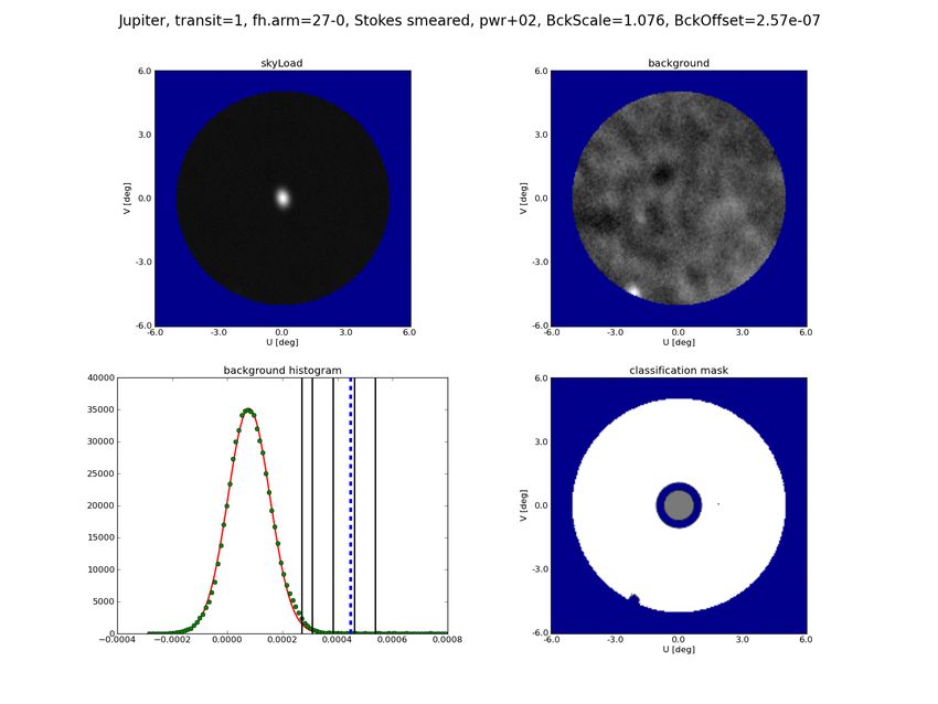
Fig. 3: Example of a map in the (u, v) reference frame for Jupiter. This image shows the first transit as seen by radiometer 27-0
(30 GHz). Top left: Map of T ant in Kcmb ranging from −4 × 10⁻⁴ Kcmb to 0.4Kcmb . Top right: Map of the background model, expressed
as T ant in Kcmb ranging from −4 × 10⁻⁴ Kcmb to 1 × 10⁻³ Kcmb . Bottom left: Histogram of T ant in Kcmb for the background. The
green points indicate the samples in the histogram, the red line indicates the best-fit Gaussian distribution, and the threshold for the
classification mask is shown by the dashed blue line. Bottom right: Classification mask. The grey region shows the planet ROI, the
white annulus is the background ROI, and the blue regions denote unused samples.
tively. Samples are plotted as a function of the radial distance Table 2: Error bars for ∆T ant,p .
between the planet and the beam centre. The blue and green points
represent samples in the planet and background ROIs, while the Planet 30 GHza 44 GHza 70 GHza
grey points represent samples not used in the fit; the best-fit model Jupiter 15 – 59 37 – 120 75 – 280
is represented by red points. The dispersion of red points as a Saturn 26 – 62 52 – 120 150 – 300
function of radial distance is mainly caused by the ellipticity of Uranus 40 – 68 63 – 130 160 – 360
Neptune 42 – 61 62 – 120 170 – 300
the beam. This did not occur for WMAP, as the WMAP team used
a symmetrized beam (Weiland et al. 2011; Bennett et al. 2013). a
Values in µKcmb .
We note that there is an apparent increase in dispersion for large
radius. This is not due to an actual increase in the variance of
the samples, but to the fact that at larger distances the population
of samples increases in size, thus widening the spanning of the a systematic error with a peak-to-peak amplitude . 10−3 Kcmb
plotted points. The LFI data for Jupiter and Saturn show a S/N (to be compared with a temperature of ≈ 0.3 Kcmb ). We chose to
that is high enough to be seen in raw data. The same does not neglect this residual, as at this stage it is not easy to understand
hold for Uranus and Neptune. whether this effect is due to uncertainties in the beam model or
bandpass or other perturbations. Moreover, the definition of a
Figure 5 shows the distribution of the residuals of the fit, new beam model for Planck/LFI is outside the purpose of this
radially averaged in constant-width bins; the bars denote the RMS paper.
of the residuals in each bin. In most cases, the radial pattern of the Figure 6 provides a summary of our measures for ∆T ant,p ∗
for
residuals is nearly flat, apart from Jupiter 24 and 27, which show the whole set of planets, transits, and radiometers. For Jupiter
Article number, page 7 of 29A&A proofs: manuscript no. aa_2020_37788_maris_et_al_v2
1.0
30 GHz - LFI27-0 44 GHz - LFI24-0 70 GHz - LFI18-0
40 100 300
30 75
200
Jupiter
20 50
10 25 100
0.8 0 0 0
10 2 10 1 100 10 2 10 1 100 60 10 2 10 1 100
15 20
10 40
Saturn
10 20
5
Tant, p [mKcmb]
0.6
0 0
0
5 10
20
20
5 10 10
Uranus
0.4
0 0 0
5 10 10
20
20
0.2 5 10 10
Neptune
0 0 0
5 10 10
0.0 20
0.0 10 2 10 1 0.2 100 100.4 2 10 1 100.60 10 2 0.8 10 1 100 1.0
Radius [deg]
Fig. 4: Antenna temperature estimates T ant for Jupiter, Saturn, Uranus, and Neptune (top to bottom) and for three radiometers
representative of the 30 GHz (left), 44 GHz (centre), and 70 GHz (right) channels, as a function of the angular distance from the beam
centre. The blue bands show the distribution of samples in the planet ROI (dark blue: 1σ region; light blue: peak-to-peak variation).
The green bands have the same interpretation, but indicate the background ROI. The grey bands show the data before having been
σ-clipped; for the case of Saturn observed by LFI27-0 a point source is present that was removed before the analysis (not present in
the green line). The separation between the blue and green lines indicates the presence of the avoidance ROI, not included in our fits.
The red line shows the best-fit model, and its width is the root mean square (RMS) of the model due to the ellipticity of the beam.
1.0
30 GHz - LFI27-0 44 GHz - LFI24-0 70 GHz - LFI18-0
2 5.0
1 2.5 5
Jupiter
0 0.0 0
1 2.5 5
0.8
2 5.0
2 10 2 10 1 100
5.0 10 2 10 1 100 10 2 10 1 100
1 2.5 5
Saturn
0 0.0 0
Tant, p [mKcmb]
0.6
1 2.5 5
2 5.0
2 5.0
1 2.5 5
Uranus
0.4
0 0.0 0
1 2.5 5
2 5.0
2 5.0
0.2 5
1 2.5
Neptune
0 0.0 0
1 2.5 5
2 5.0
0.0
0.0 10 2 10 1 0.2 100 100.4 2 10 1 100.60 10 2 0.8 10 1 100 1.0
Radius [deg]
Fig. 5: Radial pattern of residuals averaged over the whole set of transits.
Article number, page 8 of 29Maris, Romelli, Tomasi, et al.: Revised Planck/LFI 2018 planet brightness temperatures
400 Jupiter 60 Saturn Uranus 1.6 Neptune
1 5 1 5 3.0 1 5 1 5
2 6 2 6 2 6 2 6
3 7 3 7 3 7 3 7
4 4 8 4 8 1.4 4 8
350
50
2.5
1.2
300
40 2.0 1.0
250
Tant, p [×103Kcmb]
0.8
200 30 1.5
0.6
150
20 1.0 0.4
100
0.2
0.5
10
50 0.0
0.0
0 18 20 22 24 26 28 0 18 20 22 24 26 28 18 20 22 24 26 28 18 20 22 24 26 28
Radiometer ID Radiometer ID Radiometer ID Radiometer ID
Fig. 6: Values of ∆T ant,p
∗
for transits of each planet and radiometer. The X-axis is the radiometer index in form hh.p with hh = 18, 19,
20, 21, 22, 23 for the 70 GHz channel, 24, 25, 26 for the 44 GHz channel, and 27, 28 for the 30 GHZ channels. The p index accounts
for polarization with 0 for M (Y) polarization and 1 for S (X) polarization. The error bars account for noise. For Jupiter and Saturn,
they are smaller than the size of the symbols.
and Saturn the dispersion of ∆T ant,p
∗
is only partially affected by planes, varying observing conditions led to different apparent as-
random noise, which introduces a RMS scatter in ∆T ant,p ∗
of at pect ratios of the shape of the planets. In addition we have to take
−4
most a few 10 Kcmb . When converted into a relative error per care of systematics of the beam model as its numerical efficiency
planet, transit, and radiometer, the order of magnitude for Jupiter and the beam aperture. We can reduce the antenna temperature to
is 10−3 , for Saturn 10−2 , about 5 × 10⁻¹ for Uranus, and up to 1 standardized conditions, using the following formula:
for Neptune. The range of errors for our estimates are provided
in Table 2. Ω(ba)
beam /Ω̃beam (1 + faper )(1 + xη )
∆T
f ant,p = ∆T ant,p
∗
, (25)
Because of the small S/N, in some cases the signal for Uranus Ωp /Ω̃p 1 + fasp
and Neptune is consistent with zero. This occurs when the con-
fusion noise from the instrument and the background are larger where tilted quantities indicate fiducial values. For each channel
than the signal induced by the planet. Whenever this happened, we take as a fiducial value Ω̃beam , the median of the Ω(ba) beam for
we removed the affected data from our analysis. that channel from Table 1. The actual values we used are 1.006 ×
10−4 sterad (30 GHz), 8.263 × 10⁻⁵ sterad (44 GHz), and 1.607 ×
3.3. Estimation of a fiducial antenna temperature 10−5 sterad (70 GHz). Since the planet solid angle Ωp depends
on the observer-to-planet distance, |∆| (Eq. 1), the reduction to a
Figure 6 shows some variability among transits and radiometers fiducial solid angle is equivalent to reduction to a fiducial distance.
for the same planet, with a clear pattern in the variation of ∆T ant,p
∗
In Table 3, we list the values we used for planet radii, distances to
within the same frequency channel and transit. As an example, the observer, and solid angles of the planets. Several conventions
∆T ant,p
∗
for LFI20/21 is larger than for LFI19/22, which in turn is and approximations are used in the literature to measure distances
larger than for LFI18/23. The first reason for these discrepancies and solid angles. As an example, distances to Jupiter can range
is the difference in the value of Ωbeam among various radiometers from 4.04 AU to 5.2 AU. To ease comparisons, we use the same
because this value is largest for the radiometers located far from scale of distances and solid angles as WMAP (Weiland et al.
the centre of the focal plane, and produces the bent pattern of the 2011; Bennett et al. 2013). The quantity fasp in Eq. (25) is the
70 GHz channel or the jump between horn 24 and horn 25 and 26. aspect correction factor described in Sect. A.5; this accounts
Secondly, we must consider changes in the circumstances of the for the fact that the aspect ratio of the planet seen by Planck
observation among different radiometers and transits, which leads changes in time. The parameter faper is the aperture correction
to differences in the Planck–planet distance |∆| (Eq. 1), and so described in Sect. A.6, and it corrects for the loss of signal in the
in Ωp , producing the relative shift of the measurements between background ROI. The quantity xη is a correction factor for the
one transit and the other. We considered the change in |∆| among lack of numerical efficiency of the beam. As detailed in Sect. A.7,
different transits and the change occurring while observing the the limited accuracy in the numerical computation of the beam
same transit from different horns (refer to Sect. 2.1). Since planets induces a systematic in the measured fluxes at the level of ∼ 10−3 .
are not spherical and their polar axis are tilted on their orbital The precise value of xη cannot be determined precisely, but it is
Article number, page 9 of 29A&A proofs: manuscript no. aa_2020_37788_maris_et_al_v2
Table 3: Fiducial geometric parameters. Table 4: List of symbols used in Sect. 4.
Planet Raeq Rbpol ∆˜ c Ω̃dp τ(ν), ∆ν, νcent , νcent,eff Band pass, bandwidth, central frequency
[km] [km] [AU] [sterad] and effective central frequency.
∆, DP Planck-planet range and planet aspect
Jupiter 71492 66854 5.2 2.481 × 10⁻⁸ angle.
Saturn 60268 54364 9.5 5.096 × 10⁻⁹ Ωp , Ω̃p Planet solid angle and its reference
Uranus 25559 24973 19.0 2.482 × 10⁻¹⁰ value.
Neptune 24764 24341 29.0 1.006 × 10⁻¹⁰ fasp , faper , fη Corrections for planet flattening, beam
aperture and beam numerical efficiency.
a
Equatorial radius of the planet. ∆T ant Variation of antenna temperature.
b
Polar radius of the planet Tb Brightness temperature.
c
Fiducial distance of the planet. T b,rj Brightness temperature in the Rayleigh-
d
Solid angle subtended by the planet. Jeans scale.
T b,c Monochromatic brightness temperature.
T b(ba) Band-averaged brightness temperature.
in the range ± fη given in Table 1. For this reason, we did not B(ba)
ν Model band-averaged brightness.
apply the correction, thus assuming xη = 0, and we included this Bp Measured brightness.
in the overall uncertainty. We provide more details in Sect. A.7
and Sect. A.12. In the Planck Collaboration (2014d) and Planck
Collaboration (2016c), a correction factor fSL was introduced to can be used to define T b(ba) :
account for sidelobes. In this work, this correction is no longer (ba)
needed because the GRASP beam model already includes the B(ba)
ν Tb = Bp , (29)
effect of side lobes; Sect. A.8 provides more details.
Figure 7 shows the derived distribution of the values ∆T
f ant,p where B(ba)
ν (T b ) is the band-averaged SED of a Planckian black
(Eq.25). The dispersion within the same frequency channel is sig- body. Its inversion is described in Sect. A.11. Conversion among
nificantly reduced for the 70 GHz and nearly flattens, and all the the different conventions is not difficult, but a detailed model of
44 GHz radiometers are now consistent. Geometric corrections the instrument bandpass must be taken in account. To simplify the
do not affect the dispersion in 30 GHz channels significantly. comparison between our results and those from WMAP, and to
produce numbers useful for atmospheric modelling, we provide
3.4. Reduction of antenna temperatures to brightness the three quantities T b,rj , T b,c , and T b(ba) when needed7 .
temperatures Figure 8 is a summary of the channel-averaged T b(ba) for each
single transit and planet as a function of the quantity DP , the sub-
The result of our estimate is expected to be the brightness of the Planck latitude at the epoch of the observation as seen from the
planet, expressed as a brightness temperature. The brightness for planet; it represents the planet aspect angle as seen from Planck.
each radiometer and transit can be derived from ∆Tf ant,p with the Since we already include the effect of band-averaging in Eq. (26),
formula we do not need any colour-correction factor.
!(ba)
Ω̃beam dBν
Bp = ∆T
f ant,p + B(ba)
ν (T cmb ), (26)
Ω̃p dT cmb 4. Results
In comparing our results with those from WMAP, we must take in
where B(ba)
ν (T cmb ) is the correction for the blocked radiation; see account the different value of the dipole amplitude used by Planck
also Sect. A.9 and Table 1. We note that the factor Ω̃beam /Ω̃p and WMAP, as this leads to a mismatch in the absolute calibration
removes the corresponding correction for standardized observing level: the Planck team used the value APlanck = 3364 ± 2 µK
conditions. (Planck Collaboration 2014d, 2016c, 2018b), while the WMAP
We now turn to the problem of properly defining what we team used AWMAP = 3355±8 µK (Hinshaw et al. 2009). Therefore,
mean with “brightness temperature” T b , as several definitions are we scaled the WMAP estimates of T b,rj by the factor 1.002831.
available in the literature. One widely used convention is to define
Moreover, WMAP reported T b,rj rather than T b,c or T b(ba) . When
a Rayleigh-Jeans (RJ) brightness temperature as
needed, we used the WMAP bandpasses to derive T b,c or T b(ba)
Bp from T b,rj , according to the procedure outlined in Sect. A.19.
T b,rj = , (27)
Bν,rj,1 Each of the quantities T b,rj , T b,c , T b(ba) includes the correction for
blocking radiation, as explained in Sect. A.9. The definition of
where Bν,rj,1 = 2kb νcent 2
/c2 is the RJ brightness at 1 K estimated at the main symbols is provided in Table 4.
frequency νcent (see also Table 1). This is the convention followed
by WMAP (Weiland et al. 2011; Bennett et al. 2013). On the
4.1. Jupiter
other hand, when data are used to model planetary atmospheres,
it is better to define T b through the inversion of a Planckian curve Table 5 lists the seven transits of Jupiter that have been observed
(de Pater & Dunn 2003; Gibson et al. 2005; de Pater et al. 2016; by LFI; the last three transits were not considered in the analysis
Karim et al. 2018; de Pater et al. 2019b) as follows: presented by Planck Collaboration (2017). Because of a combina-
tion of factors, fewer samples have been acquired in transits 1 and
Bν (T b,c , νcent ) = Bp , (28) 4. All the transits occur near the Equator, with 0.3◦ < DP < 3.4◦
where “c” denotes one of the frequency channels 30, 44, or 7
In the abstract we followed the WMAP convention and we quoted
70 GHz. In some cases, the following band-averaged formula T b,rj as T b .
Article number, page 10 of 29Maris, Romelli, Tomasi, et al.: Revised Planck/LFI 2018 planet brightness temperatures
350 Jupiter 60 Saturn Uranus 1.6 Neptune
1 5 1 5 3.0 1 5 1 5
2 6 2 6 2 6 2 6
3 7 3 7 3 7 3 7
4 4 8 4 8 1.4 4 8
300
50
2.5
1.2
250
Reduced Tant, p [×103Kcmb]
40 2.0 1.0
200 0.8
30 1.5
150 0.6
20 1.0 0.4
100
0.2
0.5
10
50
0.0
0.0
0 18 20 22 24 26 28 0 18 20 22 24 26 28 18 20 22 24 26 28 18 20 22 24 26 28
Radiometer ID Radiometer ID Radiometer ID Radiometer ID
Fig. 7: Values of ∆T ant,p after reduction to fiducial observing conditions and standardized Ωbeam and Ωp .
Table 5: Observing conditions of Jupiter per transit.
Transit Epoch PJD_Start PJD_End Nsmp EcLon EcLat GlxLat Rh ∆ Θp DP
[deg] [deg] [deg] [AU] [AU] [arcsec] [deg]
1 2009-10-28 164.66 171.47 8421 317.4 −1.0 −40.3 5.02 4.73 41.65 0.31
2 2010-07-05 413.31 422.26 11040 2.7 −1.3 −61.4 4.97 4.71 41.85 2.56
3 2010-12-11 571.72 581.43 12104 354.2 −1.4 −61.0 4.95 4.79 41.18 2.28
4 2011-08-04 810.48 816.28 6839 39.1 −1.3 −43.2 4.95 4.82 40.93 3.68
5 2012-01-18 971.09 988.22 37035 31.0 −1.1 −48.9 4.98 4.81 41.02 3.34
6 2012-09-07 1208.18 1218.63 22852 75.1 −0.8 −13.3 5.03 4.93 40.03 3.41
7 2013-02-17 1367.85 1384.41 30724 66.7 −0.5 −20.3 5.08 4.88 40.43 3.11
(see Sect. 2.4 for the definition of DP ), so that fasp < 3 × 10⁻⁴ . so we added an uncertainty of 0.3%; the calibration uncertainty
The Galactic latitude is always negative, with transit from 1 to 5 introduces an additional 0.1% to the error budget.
between −62◦ and −40◦ , transit 6 at −13◦ , and transit 7 approxi- To derive the averaged values in Table 6, we had to consider
mately at −20◦ . The last two transits are sufficiently close to the some subtleties in the analysis; these are described in Sect. A.12.
Galactic plane to suffer larger background contamination; this Of course, averaging Bp and T b,rj is not the same as averaging T b,c
is particularly true at 30 GHz, where Jupiter is weaker and the
Galactic background is larger. Figure 8 shows no evident correla- and T b(ba) , as these are not additive quantities. A more rigorous
tions between brightness temperatures and DP . However, transits approach requires us to determine the values of T b,c and T b(ba) that
6 and 7 at 30 GHz depart significantly from the average. For this fit the observed Bp ; this can be done through the minimization
reason, we limited our analysis to the first five transits. In total of the function of merit in Eq. (A.13), Sect. A.12. We verified
there are 110 measurements (+44 in transits 6 and 7), of which that a simple average agrees with the result of a minimization
20 (+8) at 30 GHz, 30 (+12) at 44 GHz, and 60 (+14) at 70 GHz. within the second decimal figure, given the observing conditions
Table 6 reports our values for Bp , T b,rj , T b,c , and T b(ba) . We of Planck/LFI. However, the numbers we report in Table 6 were
computed these as the weighted averages of the measurements for derived using the rigorous approach.
each frequency channel across the corresponding set of radiome- Estimating uncertainties is more subtle, as several effects are
ters, still considering five transits. Adding transits 6 and 7 has a to be considered. Firstly, there is a large variability in the error
minor impact on the 70 GHz channel: T b,rj = 170.40 ± 0.16 K, bars for T b,rj , which are denoted as δrnd T b,rj : in fact, δrnd T b,rj varies
T b,c = 172.08 ± 0.16 K, T b(ba) = 171.07 ± 0.17 K. This is a 0.1 K from 0.06 K to 0.26 K (1σ), These variations can look puzzling,
reduction in temperature, and a marginal improvement on the but the transit-to-transit variability in δrnd T b,rj is highly correlated
error bars. Since we consider band-averaged quantities, we used with the number of samples √ NP in the planet ROI: the correlation
the weighted average of the individual νcent or νcent,eff of each coefficient between 1/ NP and δrnd T b,rj is ≥ 0.96. If we assume
radiometer as the reference frequency. We did not include the that the average of δrnd T b,rj across a channel is representative of
effect of the beam numerical efficiency fη (Sect. A.7) in Table 6, the uncertainties in the data, we should expect overall errors to
Article number, page 11 of 29A&A proofs: manuscript no. aa_2020_37788_maris_et_al_v2
Transit 1 Transit 2 Transit 3 Transit 4 Transit 5 Transit 6 Transit 7 Transit 8
1.0
Jupiter 138
Saturn 200
Uranus 235
Neptune
146
145 133 113 151
0.8
144
Brightness Temperature [K]
127 25 68
147 169 217
161
0.6
142 144 149
160
0.4
159 137 120 82
172 149 146 146
0.2
146
171 102 128
170
0.0 0 142 584 110
0.0 2 0.2 4 1 13 0.4 24 0.6 15 27 290.8 28 27
1.0
DP [deg]
Fig. 8: Values of channel-averaged T b(ba) per transit as a function of DP , for 30 GHz (top), 44 GHz (middle), and 70 GHz (bottom)
channels. The high variability in the estimates for Saturn is mainly due to the presence of the rings, which were not removed in this
plot.
√ √ √
be ∼ 0.12/ 28 K, ∼ 0.16/ 42 K, and ∼ 0.08/ 84 K, for the 30, be assessed. To validate our estimates for uncertainties given by
44, and 70 GHz channels, respectively. However, this is not what least-square fits, we used a bootstrap technique and a Markov
we see in Table 6, as the errors reported are of the order of 0.2 K, chain Monte Carlo (MCMC). In case of significant discrepancies,
which are comparable to the worst δrnd T b,rj on a single measure. we picked the largest error estimate.
Another indication of some possible systematic error in our Values of T b,rj , T b,c , and T b(ba) in Table 6 are very similar, with
data is the scatter of T b,rj among transits, which exceeds what differences smaller than 2 K (∼ 1 %). This happens because the
would be expected from a normal distribution with variance brightness temperature of Jupiter is greater than 140 K: since the
δrnd T b,rj
2
. The standard deviations for T b,rj are 0.800 K at 30 GHz, radiometers of Planck measure frequencies below 100 GHz the
1.072 K at 44 GHz, and 1.439 K at 70 GHz, while peak-to-peak difference between Planck’s law and the RJ approximation is not
variations are 3.38 K at 30 GHz, 4.13 K at 44 GHz, and 6.06 K at large. However, the difference exists and explains the fact that
70 GHz. Moreover, the distribution of the residuals is not Gaus- T b,rj > T b(ba) at 30 GHz and the opposite at 44 GHz and 70 GHz.
sian. In fact, below 30 GHz Planck’s law is sufficiently approximated
Fig. 7 shows that the estimates for ∆T ant at 70 GHz are dis- by the RJ law with brightness scaling as ν2 ; in this case, the band
tributed around the mean, but they are not completely compatible averaged brightness is larger than the RJ brightness computed
with random fluctuations. A closer inspection reveals that most
of the effect comes from data collected by the radiometers as- at the central frequency. Consequently, T b,rj > T b(ba) is needed to
sociated with horns 18 and 22. The averaged T b,rj from horn 18 explain the same brightness. At higher frequency, the two laws
deviates by −2.5 K from the average for 70 GHz, while for horn diverge more significantly, and the band-averaged brightness is al-
22 the deviation is +2. K; for others, the difference is less than ways lower than the RJ brightness at central frequency; therefore,
0.5 K, which is compatible with the hypothesis of random noise T b,rj < T b(ba) is needed to explain the same brightness. The critical
fluctuations. However, removing these samples does not change frequency where this swap occurs is mainly determined by the
the results in the table significantly; as an example, we obtained bandwidth: for 30 GHz and 44 GHz radiometers, the critical fre-
T b(ba) = 171.02 K instead of T b(ba) = 170.17 K (but the 1σ error quency is in the range 29–37 GHz, while for 70 GHz radiometers
decreases from 0.19 K to 0.11 K). is 53–60 GHz. The central frequencies for the 30 GHz channel
are just below the critical frequencies, while the opposite hap-
Part of the observed variability across radiometers is intrin-
pens for 44 GHz and 70 GHz radiometers, thus explaining the
sic to the source, given the relatively wide bandwidth of our
observed difference. We provide a more quantitative discussion
frequency channels, especially at 70 GHz (Planck Collaboration
in Appendix A.14.
2016c). This means that introducing some correction to flatten
this effect would introduce another kind of distortion in the data. In Fig. 9 we plot the estimates for T b(ba) reported in Table 6 and
However when computing uncertainties on channel averaged compare these with a selection of results and models available
quantities, the adequacy of usual error propagation formula must in the literature. Points are plotted at νcent for each frequency
Article number, page 12 of 29Maris, Romelli, Tomasi, et al.: Revised Planck/LFI 2018 planet brightness temperatures
Table 6: Channel-averaged resultsa for Jupiter, excluding transits 6 and 7.
b
ch νcent νcent,eff Bp b T b,rj b T b,c b T b(ba)
[GHz] [GHz] [MJy/sr] [K] [K] [K]
30 28.40 28.43 3598.2 ± 16.4 144.93 ± 0.17 145.62 ± 0.17 144.69 ± 0.19
44 44.10 44.16 9570.0 ± 23.0 159.76 ± 0.19 160.82 ± 0.19 160.27 ± 0.19
70 70.40 70.36 25866.0 ± 127.8 170.50 ± 0.18 172.18 ± 0.18 171.17 ± 0.19
a
The effect of fη is not included.
b
The value includes blocked radiation.
180 b.p. 30 GHz b.p. 44 GHz b.p. 70 GHz
170
160
Tb [K]
150
140 Planck/LFI Tb(ba) Karim + (2018)
WMAP Tb(ba) dePater + (2019a)
Joiner and Steffes (1991) Karim et al. (2018) Best Fit Model
Greve + (1994) Karim et al. (2018) + Sync
Gibson + (2005)
130
30 40 50 60 70 80 90
Central Frequency [GHz]
Fig. 9: Comparison of Jupiter measurements made in this paper (red circles) with WMAP (black points, taken from (Weiland et al.
2011; Bennett et al. 2013) and converted to T b(ba) ) and with measurements from literature and the RT model by Karim et al. (2018).
The model brightness temperature T b(RT) is plotted as a dark grey line. The top and bottom dashed lines represent the upper and lower
limits of model uncertainties as provided in the same paper. The RT model plus the synchrotron emission correction is plotted as a red
line; the grey band represents the lower and upper limits. For references of ground-based measurements, see the text. The brightness
temperatures reported by Gibson et al. (2005) are recalibrated measures originally published by Klein & Gulkis (1978). The violin
plots at the top of the figure represent the relative sensitivity to the frequencies inside each bandpass.
channel. The violin plots at the top give insight into how τ(ν) Apart from WMAP, Fig. 9 compares our estimates with other
changes within each frequency channel. The quoted error bars are results found in the literature. The few measurements above
comparable with the size of the symbols, even including the effect 40 GHz are consistent with our estimates; the error bars are how-
of the ±0.3% fη correction uncertainty. The black points in the ever large, and the consistency is therefore of little significance.
figure represent the WMAP measurements, taken from Weiland Below 40 GHz, the situation is much better. In particular, the
et al. (2011) and Bennett et al. (2013), and converted to T b(ba) as CARMA measurements in Karim et al. (2018) cover the 27.7–
detailed at the begin of this section and in Sect. A.19. The WMAP 34.7 GHz fairly well. Our estimate at 30 GHz is consistent with
results compare well with ours. The plot includes measurements CARMA, but we see an excess in T b(ba) of nearly 2 K. As we
taken from8 Joiner & Steffes (1991), Greve et al. (1994), Gibson explain below, this excess is likely due to the presence of a syn-
et al. (2005), Karim et al. (2018) and de Pater et al. (2019a). The chrotron contribution to the Jupiter signal that has been removed
results from Gibson et al. (2005) are measures provided by Klein in the CARMA data (Karim et al. 2018).
& Gulkis (1978) (Tab.II in the paper) and reprocessed. According
The sparse frequency coverage of measurements in the litera-
to the conventions used in this paper they are similar to T b,c .
ture makes it difficult to quantitatively compare our measurements
8
Results from de Pater et al. (1982) and Goldin et al. (1997) are not with those of other authors without adopting an interpolation
included, as they are outside the frequency range of interest. scheme. But microwave emission of Jupiter cannot be reduced to
Article number, page 13 of 29You can also read