Synthetic Galaxy Clusters and Observations Based on Dark Energy Survey Year 3 Data - arXiv
←
→
Page content transcription
If your browser does not render page correctly, please read the page content below
DES-2020-0629
FERMILAB-PUB-21-049-AE

                                                  Mon. Not. R. Astron. Soc. 000, 1–21 (2021)           Printed 23 February 2021   (MN LATEX style file v2.2)

                                                  Synthetic Galaxy Clusters and Observations Based on Dark Energy
                                                  Survey Year 3 Data

                                                   T. N. Varga,1,2? D. Gruen,3,4,5 S. Seitz,1,2 N. MacCrann,6 E. Sheldon,7 W. G. Hartley,8 A. Amon,4
                                                   A. Choi,9 A. Palmese,10,11 Y. Zhang,10 M. R. Becker,12 J. McCullough,4 E. Rozo,13 E. S. Rykoff,4,5
                                                   C. To,3,4,5 S. Grandis,14 G. M. Bernstein,15 S. Dodelson,16 K. Eckert,15 S. Everett,17 R. A. Gruendl,18,19
                                                   I. Harrison,20,21 K. Herner,10 R. P. Rollins,21 I. Sevilla-Noarbe,22 M. A. Troxel,23 B. Yanny,10
   arXiv:2102.10414v1 [astro-ph.CO] 20 Feb 2021

                                                   J. Zuntz,24 H. T. Diehl,10 M. Jarvis,15 M. Aguena,25,26 S. Allam,10 J. Annis,10 E. Bertin,27,28
                                                   S. Bhargava,29 D. Brooks,30 A. Carnero Rosell,31,26,32 M. Carrasco Kind,18,19 J. Carretero,33
                                                   M. Costanzi,34,35,36 L. N. da Costa,26,37 M. E. S. Pereira,38 J. De Vicente,22 S. Desai,39 J. P. Dietrich,14
                                                   I. Ferrero,40 B. Flaugher,10 J. García-Bellido,41 E. Gaztanaga,42,43 D. W. Gerdes,44,38 J. Gschwend,26,37
                                                   G. Gutierrez,10 S. R. Hinton,45 K. Honscheid,9,46 T. Jeltema,17 K. Kuehn,47,48 N. Kuropatkin,10
                                                   M. A. G. Maia,26,37 M. March,15 P. Melchior,49 F. Menanteau,18,19 R. Miquel,50,33 R. Morgan,51
                                                   J. Myles,3,4,5 F. Paz-Chinchón,18,52 A. A. Plazas,49 A. K. Romer,29 E. Sanchez,22 V. Scarpine,10
                                                   M. Schubnell,38 S. Serrano,42,43 M. Smith,53 M. Soares-Santos,38 E. Suchyta,54 M. E. C. Swanson,18
                                                   G. Tarle,38 D. Thomas,55 and J. Weller1,2
                                                                                                                    (DES Collaboration)

                                                   Author affiliations are listed at the end of this paper.

                                                  23 February 2021

                                                                                              ABSTRACT
                                                                                              We develop a novel data-driven method for generating synthetic optical observations of galaxy
                                                                                              clusters. In cluster weak lensing, the interplay between analysis choices and systematic effects
                                                                                              related to source galaxy selection, shape measurement and photometric redshift estimation can
                                                                                              be best characterized in end-to-end tests going from mock observations to recovered cluster
                                                                                              masses. To create such test scenarios, we measure and model the photometric properties of
                                                                                              galaxy clusters and their sky environments from the Dark Energy Survey Year 3 (DES Y3)
                                                                                              data in two bins of cluster richness λ ∈ [30; 45), λ ∈ [45; 60) and three bins in cluster
                                                                                              redshift (z ∈ [0.3; 0.35), z ∈ [0.45; 0.5) and z ∈ [0.6; 0.65). Using deep-field imaging data
                                                                                              we extrapolate galaxy populations beyond the limiting magnitude of DES Y3 and calculate
                                                                                              the properties of cluster member galaxies via statistical background subtraction. We construct
                                                                                              mock galaxy clusters as random draws from a distribution function, and render mock clusters
                                                                                              and line-of-sight catalogs into synthetic images in the same format as actual survey obser-
                                                                                              vations. Synthetic galaxy clusters are generated from real observational data, and thus are
                                                                                              independent from the assumptions inherent to cosmological simulations. The recipe can be
                                                                                              straightforwardly modified to incorporate extra information, and correct for survey incom-
                                                                                              pleteness. New realizations of synthetic clusters can be created at minimal cost, which will
                                                                                              allow future analyses to generate the large number of images needed to characterize system-
                                                                                              atic uncertainties in cluster mass measurements.
                                                                                              Key words: cosmology: observations, gravitational lensing: weak, galaxies: clusters: general

                                                                                                                                    1   INTRODUCTION
                                                  ?   corresponding author: t.varga@campus.lmu.de

                                                                                                                                    The study of galaxy clusters has in recent years became a prominent
                                                                                                                                    pathway towards understanding the nonlinear growth of cosmic
                                                                                                                                    structure, and towards constraining the cosmological parameters of

                                                  © 2021 RAS
2      T. N. Varga

the universe (Allen et al. 2011; Kravtsov & Borgani 2012; Wein-           underlying model. A mass model calibrated by McClintock et al.
berg et al. 2013). Weak gravitational lensing provides a practical        2019 is used to imprint a realistic lensing signal on background
method to study the mass properties of clusters. It relies on estimat-    galaxies, which will enable future studies to perform end-to-end
ing the gravitational shear imprinted onto the shapes of background       tests for recovering cluster masses from a weak lensing analysis of
source galaxies. The lensing effect is directly connected to the grav-    synthetic images, incorporating photometric processing, shear and
itational potential of the lens, and its measurement is readily scal-     photometric redshift measurement and systematic calibration for
able to an ensemble of targets in wide-field surveys (Bartelmann          lensing profiles and maps in a fully controlled environment. This is
& Schneider 2001). For this reason the lensing based mass calibra-        different from insertion based methods (Suchyta et al. 2016, Everett
tion of galaxy clusters has become a standard practice for galaxy         & Yanny et al., 2020), where synthetic galaxies are added onto real
cluster based cosmological analyses (Rozo et al. 2010; Mantz et al.       observations: Our method involves a generalization step avoiding
2015; Planck Collaboration 2016; Costanzi et al. 2019; Bocquet            re-using identical clusters multiple times, the full control of syn-
et al. 2019; DES Collaboration 2020).                                     thetic data allows quantifying the specific impact of the different
      Methods for estimating the shapes of galaxies include model         cluster properties on the lensing measurement.
fitting and measurements of second moments, with several innova-                The primary focus of this work is to present the algorithm and
tive approaches developed in recent literature (Zuntz et al. 2013;        a pilot implementation for generating synthetic cluster observations
Refregier & Amara 2014; Miller et al. 2013; Bernstein & Arm-              for the DES Y3 observational scenario mimicking the stacked lens-
strong 2014; Huff & Mandelbaum 2017; Sheldon & Huff 2017;                 ing strategy of McClintock & Varga et al., (2019) and DES Col-
Sheldon et al. 2020). Irrespective of the chosen family of algo-          laboration (2020). Due to the transparent nature of the framework,
rithms, the performance of the shear estimates cannot be a-priori         changes and improvements aiming for increased realism: e.g. cor-
guaranteed, and needs to be validated in a series of tests (Jarvis        rections for input photometry incompleteness or high resolution,
et al. 2016, Fenech Conti et al. 2017, Zuntz & Sheldon et al.,            deep cluster imaging, can be directly added to the model in fu-
2018, Samuroff et al. 2018, Mandelbaum et al. 2018, Kannawadi             ture studies. For this reason, the presented algorithm is expected to
et al. 2019). These rely on synthetic observations: image simula-         be easily generalized and expanded to other ongoing (HSC: Hy-
tions which are then used to estimate the bias and uncertainty of         per Suprime-Cam1 , KiDS: Kilo-Degree Survey2 ) and upcoming
the different methods in a controlled environment (Massey et al.          (LSST: Legacy Survey of Space and Time3 , Euclid4 , Nancy Grace
2007; Bridle et al. 2009; Mandelbaum et al. 2015; Samuroff et al.         Roman Space Telescope5 ) weak lensing surveys as well.
2018; Kannawadi et al. 2019; Pujol et al. 2019; MacCrann et al.                 The structure of this paper is the following: In Section 2 we
2020).                                                                    introduce the DES year 3 (Y3) dataset, in Section 3 we outline the
      Galaxy clusters present a unique challenge for validating weak      statistical approach used in modeling the synthetic lines-of-sight,
lensing measurements for a multitude of reasons: they deviate from        in Section 4 we describe the concrete results of the galaxy dis-
the cosmic median line-of-sight in terms of the abundance and             tribution models derived from the DES Y3 dataset, and finally in
properties of cluster member galaxies (Hansen et al. 2009; To et al.      Section 5 we outline the method for generating mock observations
2019) resulting in increased blending among light sources (Simet &        for DES Y3. In the following we assume a flat ΛCDM cosmology
Mandelbaum 2015; Euclid Collaboration 2019; Eckert et al. 2020,           with Ωm = 0.3 and H0 = 70 km s–1 Mpc–1 , with distances defined
Everett & Yanny et al., 2020), host a diffuse intra-cluster light (ICL)   in physical coordinates, rather than comoving.
component (Zhang et al. 2019; Gruen et al. 2019; Sampaio-Santos
et al. 2020; Kluge et al. 2020) influencing photometry, and induce
characteristically stronger shears at small scales (McClintock &          2    DES Y3 DATA
Varga et al., 2019).
      In this study we create synthetic galaxy clusters, and optical      The first three years of DES observations were made between
observations of these synthetic galaxy clusters in an unsupervised        August 15, 2013 and February 12, 2016 (DES Collaboration
way from a combination of observational datasets. To achieve this,        2016; Sevilla-Noarbe et al. 2020). This Y3 wide-field dataset has
we measure and model the average galaxy content of redMaPPer              achieved nearly full footprint coverage albeit at shallower depth,
selected galaxy clusters in Dark Energy Survey Year 3 (DES Y3)            with on average 4 tilings in each band (g, r, i, z) out of the eventu-
data along with the measurement and model for galaxies in the fore-       ally planned 10 tilings. From the full 5000 deg2 , the effective sur-
ground and background. During this procedure the DES Y3 wide-             vey area is reduced to approximately 4400 deg2 due to the mask-
field survey (Sevilla-Noarbe et al. 2020) is augmented with infor-        ing of the Large Magellanic Cloud and bright stars. In parallel to
mation from deep-field imaging data (Hartley & Choi et al., 2020),        the wide-field survey a smaller, deep field survey is also conducted
resulting in enhanced synthetic catalog depth and better resolved         covering a total unmasked area of 5.9 deg2 in 4 patches (Hartley
galaxy features. Each synthetic cluster and its line-of-sight is gen-     & Choi et al., 2020). These consist of un-dithered pointings of the
erated as a random draw from a model distribution, which enables          Dark Energy Camera (DECam, Flaugher et al. 2015) repeated on a
creating the large numbers of mock cluster realizations required          weekly cadence, resulting in data 1.5 - 2 mag deeper than the wide-
for benchmarking precision measurements. This approach short-             field survey. The DES Y3 footprint is shown on Figure 1. We use
cuts the computational cost and limited representation of reality of      three of the four of DES Y3 Deep Fields denoted as SN-C, SN-E
numerical simulations. The synthetic catalogs of cluster member           and SN-X, These consist of 8 partially overlapping tilings: three
galaxies and foreground and background galaxies along with the            tilings for SN-C and SN-X, and two of the SN-E. Their location is
small-scale model for light around the cluster centers are then ren-      also shown on Figure 1.
dered into images in the same format as actual survey observations        1   http://hsc.mtk.nao.ac.jp/ssp/
and can be further processed with the standard data reduction and         2   http://kids.strw.leidenuniv.nl/index.php
analysis pipelines of the survey.                                         3   https://www.lsst.org/
      The synthetic cluster images are controlled environments,           4   http://sci.esa.int/euclid/
where all light can be traced back to a source specified in the           5   https://wfirst.gsfc.nasa.gov/

                                                                                                                     © 2021 RAS, MNRAS 000, 1–21
Synthetic Galaxy Clusters and Observations Based on Dark Energy Survey Year 3 Data                                                           3
                                   RA
              60      45     30     15      0      345      330
      +15                                                         0.00225
                   SN-X                                           0.00200
        0
            SN-C                                                  0.00175

                                                                         nc [arcmin 2]
       15                                                         0.00150
                                         SN-E
DEC

                                                                  0.00125
       30                                                         0.00100
                                                                  0.00075
       45                                                         0.00050

Figure 1. Footprint of targeted clusters in DES Y3. Blue markers: location
of Deep field regions SN-C, SN-E, SN-X (marker size not to scale). The
colorscale indicates the number density of galaxy clusters (nc ) identified by
the redMaPPer algorithm.

2.1     Wide-field data                                                                  Figure 2. Distribution of redMaPPer clusters in DES Y3 dataset in the
                                                                                         volume-limited sample. Solid black rectangles: narrow redshift selection.
The primary photometric catalog of DES Y3 is the Y3A2 GOLD
                                                                                         Blue dotted rectangles: DES Y1 cluster cosmology selection.
dataset (Sevilla-Noarbe et al. 2020). This includes catalogs of pho-
tometric detections and parameters from the wide-field survey as
well as the corresponding maps of the characteristics of the obser-                      SOF photometry catalog described above, from which redMaPPer
vations, foreground masks, and star-galaxy classification.                               identifies galaxy clusters as overdensities of red-sequence galaxies.
      Data processing starts with single epoch images for which de-                      This analysis uses redMaPPer version v6.4.22+2. An optical mass
trending and photometric corrections are applied. They are sub-                          proxy richness λ is assigned to each cluster defined by the effec-
sequently co-added to facilitate the detection of fainter objects.                       tive number of red-sequence member galaxies brighter than 0.2 L∗ .
The base set of photometric detections is obtained via SExtrac-                          Cluster redshifts are estimated based on the photometric redshifts
tor (Bertin & Arnouts 1996) from r + i + z coadds. The fiducial                          of likely cluster members yielding a nearly unbiased estimate with
photometric properties for these detections are derived using the                        a scatter of σz /(1 + z) ≈ 0.006 (McClintock & Varga et al., 2019).
single-object-fitting (SOF) algorithm based on the ngmix (Shel-                                We consider a locally volume-limited sample of clusters ex-
don 2015) software which performs a simultaneous fit of a bulge +                        tending up to z ≈ 0.65, set by the survey completeness depth
disk composite model (CModel, cm) to all available exposures of                          of i ≈ 22.6. This redMaPPer cluster catalog contains more than
a given object while modelling the point spread function (PSF) as                        869,000 clusters down to λ > 5 and more than 21,000 above
a Gaussian mixture for each exposure. An expansion of this model                         λ > 20. The spatial distribution of the latter higher richness sample
is the multi-object-fitting (MOF) (Sevilla-Noarbe et al. 2020) ap-                       is shown on Figure 1, and the richness and redshift distribution is
proach where in addition to the above first step friends-of-friends                      shown on Figure 2. In addition to the cluster catalog, a catalog of
(FoF) groups of galaxies are identified based on their fiducial mod-                     reference random points is also provided, which are drawn from the
els, and in a subsequent step the galaxy models are corrected for                        part of the footprint where survey conditions permit the detection
all members of a FoF group in a combined fit. While for the Y3A2                         of a cluster of given richness and redshift.
GOLD dataset the SOF and MOF photometry were found to yield                                    Finally we note that redMaPPer uses SOF derived photomet-
similar solutions, it is expected that in crowded environments the                       ric catalogs instead of MOF, however this is expected to have no
MOF photometry would perform better, due to its more advanced                            impact on the result of this work as we only utilize the positions,
treatment of blending.                                                                   richnesses and redshifts of the clusters.
      The 10σ detection limit for galaxies using SOF photometry in
the Y3A2 catalog is g = 23.78, r = 23.56, i = 23.04, z = 22.39 de-
fined in the AB system (Sevilla-Noarbe et al. 2020). That is a 99 per                    2.3   Deep-Field Data
cent completeness for galaxies with i < 22.5. Star - galaxy separa-                      The DES supernova and deep field survey is organized into four dis-
tion is performed based on the morphology derived from SOF and                           tinct fields: SN-S, SN-X, SN-C and SN-E (Kessler et al. 2015; Ab-
MOF quantities, which for the i < 22.5 sample has 98.5 per cent ef-                      bott et al. 2019,Hartley & Choi et al., 2020). In this work we only
ficiency and 99 per cent purity, yielding approximately 226 million                      consider the SN-X, SN-C, SN-E fields covering a total unmasked
extended objects out of a base sample of 390 million detections.                         area of 4.64 deg2 which overlap with the VISTA Deep Extragalac-
SOF and MOF derived magnitudes are corrected for atmospheric                             tic Observations (VIDEO) survey (Jarvis et al. 2013), providing
and instrumental effects and for interstellar extinction to obtain the                   J, H, K band coverage.
final corrected magnitudes.                                                                    In the present study we consider only the detections derived
                                                                                         from the COADD_TRUTH stacking strategy which aims to opti-
                                                                                         mize for reaching approximately 10× the wide-field survey depth
2.2     RedMaPPer Cluster Catalog
                                                                                         while requiring that the deep field resolution (FWHM) be no worse
We consider an optically selected sample of galaxy clusters iden-                        that the median FWHM in the wide-field data (Hartley & Choi
tified by the redMaPPer algorithm in the DES Y3 data (Rykoff                             et al., 2020).
et al. 2014). The base input for this cluster finding is the Y3A2                              A difference compared to Y3A2 GOLD is that the MOF al-

© 2021 RAS, MNRAS 000, 1–21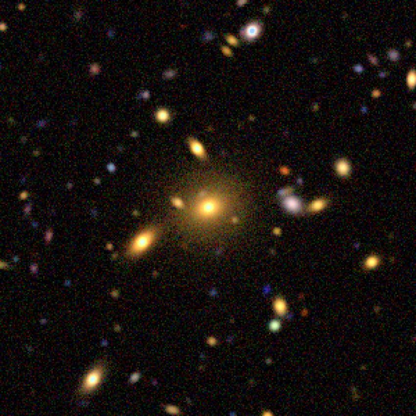
4           T. N. Varga

          400
          350       RA: 3.3305 deg        DEC: -41.2431 deg
          300
                     =46.70
                    z=0.33
          250
y [pix]

          200
          150
          100
           50
            0
                    DES Y3
          400
          350
          300
          250
y [pix]

          200
          150       Synthetic DES
          100                                                                                                                       0.5 arcmin
                       [45; 60)
           50       z [0.3; 0.35)                                                                                                   100 kpc
            0
          400
          350
          300
          250
y [pix]

          200
          150          cluster i = 17.4
          100          cluster i = 24.5
                       field i = 17.4
           50          field i = 24.5
            0
          400
          350
          300
          250
y [pix]

          200
          150          cluster z = 0.325
          100          foreground z < 0.325
                       background z > 0.9
           50          background z = 0.4
            0
                0             200             400             600                800              1000              1200               1400              1600
                                                                              x [pix]
Figure 3. Real and synthetic galaxy cluster side by side. Top: gri color composite image of a real redMaPPer galaxy cluster in the DES Y3 footprint. Second
row: gri color composite image of a synthetic galaxy cluster representative of λ ∈ [45 60), z ∈ [0.3; 0.35). Third row: brightness distribution of the synthetic
light sources for cluster members (red/brown) and foreground and background objects (blue). Darker shades and larger symbols correspond to brighter objects.
Bottom row: exaggerated shear map of background sources (red ellipses) with the shade representing redshift, cluster members (black) and foreground sources
(green).

gorithm is run with "forced photometry" where astrometry and de-                   Fig. 12 of Hartley & Choi et al., 2020). Additionally, for the deep
blending is done using DECam data, and infrared bands incorpo-                     field photometry the ngmix algorithm is run using the bulge + disk
rated only for the photometry measurement. This approach results                   composite model with fixed size ratio between the bulge and disk
in a coadded consistent photometric depth of i = 25 mag. The pho-                  components (in the following denoted as bdf to distinguish from
tometric performance of these solutions were compared between                      the wide-field processing).
the DES wide and deep field datasets using a joint set of photomet-
ric sources, finding very good agreement on the derived colors (see                      A photometric redshift estimate is derived by Hartley & Choi
                                                                                   et al., (2020) for the deep-field galaxies via the EAzY algorithm

                                                                                                                             © 2021 RAS, MNRAS 000, 1–21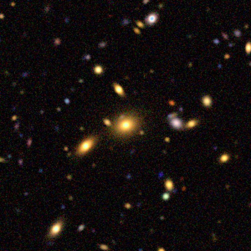
Synthetic Galaxy Clusters and Observations Based on Dark Energy Survey Year 3 Data                                                   5

(Brammer et al. 2008). These photometric redshift estimates are                  clusters of richness λ and redshift z. These distributions cannot be
obtained by fitting a mixture of stellar population templates to                 directly measured from the DES wide-field survey as individual
the ugrizJHK band fluxes of the deep field galaxies. The possible                cluster member galaxies cannot be identified with sufficient com-
galaxy redshifts and stellar template parameters are varied jointly              pleteness from photometric data alone, and the bulk of the galaxy
to obtain a redshift probability density function. The redshift esti-            populations lie beyond the completeness threshold magnitude of
mates are validated using a reference set of spectroscopic galaxy                i ≈ 22.5, where photometric errors come to dominate the de-
redshifts over the same footprint, and Hartley & Choi et al., (2020)             rived features. To counteract this limitation we adopt a two-step
finds overall good performance for bright and intermediate depths                approach: First a target distribution of well measured reference fea-
which however deteriorates into a very large outlier fraction for the            tures, in this case a set of reference colors and radius (cref ; R | λ, z)
faintest galaxies (i > 24). In light of this we note that our algorithm          is measured in the wide-field survey (Section 3.2 and Section 3.3).
for modeling the properties of cluster member galaxies presented                 In the second step the wide-field target distribution is used as a
in this analysis does not rely on redshifts, and we consider pho-                prior for resampling the galaxy features measured in the DES Deep
tometric redshifts only for describing the line-of-sight distribution            Fields (Section 3.5). Comparing the target distribution around clus-
of foreground and background galaxies. Due to the substantially                  ters and around a set of reference random points enables us to iso-
shallower limiting depth of the DES Y3 wide-field survey the im-                 late the feature distribution of cluster members (Section 3.6). Thus
pact of the increased fraction of very faint (i>24) redshift outliers            the resampling transforms the deep-field feature distribution into an
is expected to be negligible.                                                    estimate on the full feature distribution of cluster member galax-
                                                                                 ies, while keeping additional features measured accurately only in
                                                                                 the deep-field data, and extrapolate the cluster population to fainter
3     STATISTICAL MODEL                                                          magnitudes.
                                                                                       Figure 3 shows an illustration of a mock cluster generated as
3.1     Analysis Choices                                                         a result of this analysis at the level of a galaxy catalog and also as
The focus of this study is to measure and model the galaxy content               a fully rendered DES Y3-like coadd image, along with an actual
of redMaPPer selected galaxy clusters within a bin of cluster prop-              redMaPPer cluster taken from the DES Y3 footprint with similar
erties, and to use this measurement to create mock galaxy clusters.              richness and redshift.
The cluster member model is complemented by a measurement and
model for the properties of foreground and background galaxies.
Each mock cluster is constructed to be representative in terms of
                                                                                 3.2   Data Preparation
its member galaxies of the whole bin of cluster properties, and do
not aim to capture cluster-to-cluster or line-of-sight to line-of-sight          We group galaxy clusters into two bins of richness λ ∈ [30; 45) and
variations.                                                                      [45; 60), and three bins of redshift z ∈ [0.3; 0.35), [0.45; 0.5) and
      By construction, the clusters identified by redMaPPer are al-              0.6; 0.65), where each sample is processed separately. Our binning
ways centered on a bright central galaxy (BCG). Central galaxies                 scheme is motivated by the selections of McClintock & Varga et al.,
form a unique and small subset of all galaxies, and therefore we                 (2019) and DES Collaboration (2020), shown on Figure 2. In this
treat them separately from non-central galaxies. In our synthetic                pathfinder study, however, we only cover their central richness bins,
observations we consider for each cluster bin a mock central galaxy              and enforce a narrower redshift selection to reduce the smearing of
which has the mean properties of the observed redMaPPer BCG                      observed photometric features (e.g. red sequence) due to mixing
properties within that bin. In this study, we only consider clusters             of different redshift cluster members. While this smearing is not a
selected on richness and redshift (mimicking DES Collaboration                   limitation for the presented model, reduced smearing and redshift
2020), and do not aim to incorporate correlated scatter between ad-              mixing will enable useful sanity checks in evaluating performance.
ditional observables and mass properties at fixed selection. Thus the                  The base dataset for this study is a subset of the Y3A2
task for the rest of this section is to model the properties and distri-         GOLD photometric catalog selected via the flags listed in Table A2,
bution of non-central, foreground and background galaxies, in the                queried from the DES Data Management system (DESDM, Mohr
following simply denoted as galaxies. Faint stars are treated in the             et al. 2008). The flags are chosen to yield a high-completeness
same framework as foreground galaxies, while bright stars, tran-                 galaxy sample while excluding photometry failures. For each clus-
sients, streaks, and other imperfections which are masked during                 ter in a given cluster selection we select all entries from this base
data processing are not incorporated in this model6 .                            catalog which are within a pre-defined search radius θquery ≈ 6 deg
      Throughout this analysis we assume that galaxies are to first              around the cluster using the HEALPix algorithm (Górski et al.
order sufficiently described by a set of observable features, primar-            2005).
ily provided by the DES photometric processing pipeline. The key                       Directly manipulating the above dataset is not feasible, there-
features are: i-band magnitude mi with de-reddening and other rel-               fore we select a weighted, representative subsample of entries: First
evant photometric corrections applied, colors c = (g – r, r – i, i – z),         we measure the total radial number profile of galaxies around the
galaxy redshift zg , and morphology parameters s describing the                  clusters in radial bins arranged as [10–3 ; 0.1) arcmin, and in 50
scale radius, ellipticity and flux ratio of the two components of the            consecutive logarithmically-spaced radial bins between 0.1 arcmin
ngmix SOF/MOF bulge + disk galaxy model. The full list of fea-                   and 100 arcmin. Then, from each radial range we draw Ndraw =
tures and their relation to the DES Y3 data products is listed in                min(Nbin ; Nth ) galaxies where Nbin is the number of galaxies in the
Table A1.                                                                        radial bin, and Nth = 10000 is a threshold number.
      Our aim is to model the distribution of cluster member galax-                    The random draws are equally partitioned across the Nclust
ies, and foreground and background galaxies in the space of the                  clusters7 . To account for the number threshold Nth , for each drawn
above features as a function of projected separation R from galaxy
                                                                                 7 That is from the vicinity of each cluster approximately N
                                                                                                                                              draw / Nclust
6   Nevertheless, these can be added after the synthetic images are generated.   galaxies are drawn without replacement from each radial bin.

© 2021 RAS, MNRAS 000, 1–21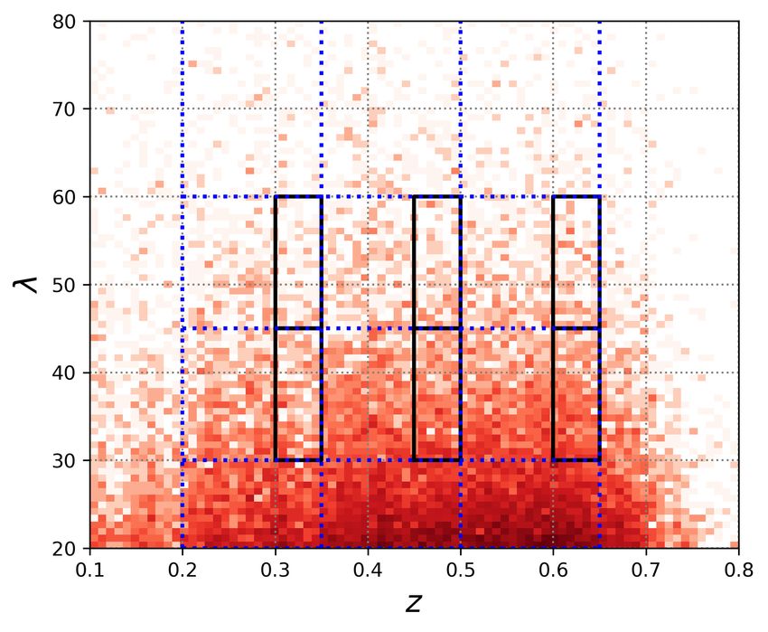
6      T. N. Varga

galaxy a weight                                                            galaxy into a set of eigenfeatures. Finally, these are standardized
                                                                           by dividing each eigenfeature by its estimated standard deviation
                          wbin = Nbin /Ndraw                        (1)    among the sample.
is assigned. Therefore the number of tracers representing the galaxy             In order to find the optimal bandwidth h for each KDE, we
distribution is reduced in an adaptive way. For each selected galaxy       perform k-fold leave-one-out cross-validation (Hastie et al. 2001).
the full catalog row is transferred from the GOLD catalog, and             Here the same base data is split into k equal parts, and from
through the random draws the same galaxy can enter multiple                these each part is once considered as the test data, and the re-
times, but at different radii.                                             mainderPis used as the training data. In this approach the score
      The outcome of the above is a galaxy photometry catalog con-         S = N1 N   j ln pn (xj , h) is calculated k = 5 times on different train-
taining the projected radius R of each entry measured from the tar-        ing and test combinations, and from this a joint cross-validation
geted cluster sample with a weight for each entry. The measurement         score is estimated. The final KDE is then constructed from the full
is repeated for a sample of reference random points selected in the        dataset using the bandwidth maximizing the cross-validation score.
same richness and redshift range as the cluster sample. This second              Using PCA standardization, bandwidths can be expressed rel-
dataset is representative of the field galaxy distributions, however,      ative to the standard deviation σ = 1 of the various standardized
through the spatial and redshift distribution of the reference random      eigenfeatures. Based on this we evaluate the cross validation score
points it also incorporates the impact of survey inhomogeneities           on a logarithmically-spaced bandwidth grid from 0.01σ to 1.2σ for
and masking.                                                               each KDE constructed. We find that h = 0.1σ simultaneously pro-
      Foreground stars appear in the projected vicinity of each            vides a good bandwidth estimate for the deep-field and the wide-
galaxy cluster on the sky and also within the deep-field areas,            field KDEs, for this reason we adopt it as a global bandwidth for
and enter into the photometry dataset. The model presented in this         further calculations.
study is not dependent on separation between stars and galaxies,
as stars are automatically removed during statistical background           3.4   Cluster and Field Population Estimates
subtraction. Nevertheless, the photometric properties of stars com-
pared to galaxies increases the computational cost, as the difference      Our aim is to model the radial feature distribution of cluster mem-
between the proposal and target distribution increases when large          ber galaxies for different samples of galaxy clusters. These must
number of stars are included. To counteract this we employ a size–         be separated from the distribution of foreground and background
luminosity cut i – mag < –50 + log10 (1 + T) + 22 to remove the bulk       galaxies which we expect to be similar to the galaxies of the mean
of the stellar population, where T is the effective size of a detection    survey line-of-sight. The input data product for the following cal-
defined as listed in Table A1. These objects will be re-added at a         culations is the feature PDF estimated from the various deep-field
later stage to produce survey-like observations.                           and wide-field galaxy catalogs for each using the KDE approach
                                                                           in Section 3.3. The full list of feature definitions are shown in Ta-
                                                                           ble A1.
3.3   Kernel Density Representation of Survey Data                               Photometric redshift estimates available for the DES wide-
                                                                           field (Hoyle & Gruen et al., 2018; Myles & Alarcon et al., 2020)
Our aim is to generalize the features of a finite set of observed          are not precise enough to isolate a sufficiently pure and complete
galaxies into an estimate on their multivariate feature probability        sample of cluster member galaxies across the full range of galaxy
density function (PDF). We achieve this task via kernel density            populations (e.g. not only the red sequence). Therefore, to avoid
estimation (KDE), which is a type of unsupervised learning algo-           the above limitation, we perform a statistical background subtrac-
rithm (Parzen 1962; Hastie et al. 2001). In brief, the finite set of       tion (Hansen et al. 2009) to estimate the feature distribution of pure
data points are convolved with a Kernel function K(r, h), where h          cluster member galaxies. In this framework we describe the line-
is the bandwidth which sets the smoothing scale during the PDF             of-sight galaxy distribution around galaxy clusters pclust as a two-
reconstruction. We adopt a multivariate Gaussian kernel function           component system of a cluster member population pmemb , and a
K(r, h) formulated for d dimensional data with a single bandwidth          field population which is approximated by the distribution around
h equal to the standard deviation. This way gaps and undersampled          reference random points prand . This yields
regions are modeled to have non-zero probability. For the practical
calculation of KDEs we make use of the scikit-learn imple-                                           n̂r     n̂c
                                                                                  pmemb (θ, R) =                 pclust (θ, R) – prand (θ, R)   (2)
mentation of the above algorithm8 .                                                               n̂c – n̂r n̂r
     The photometry catalog has features with very disparate               where in practice both p.d.f-s on the right hand side are KDEs con-
scales9 . This means that any single bandwidth h (smoothing scale)         structed from the wide-field dataset, θ is the list of features consid-
is not equally applicable for all dimensions. To address this we           ered, and R is the projected separation from the targeted positions
standardize and transform the input features before the KDE step           on the sky. n̂c and n̂r refer to the mean number of galaxies detected
into a set of new features which are better described by a single          within Rmax around clusters and random points.
bandwidth parameter. First we subtract the mean of each feature,                 The above approach is only applicable for those features θ
then perform a principle component analysis (PCA) to find the              and their respective value ranges which are covered by the wide-
eigendirections of the input features (Hastie et al. 2001) via the         field dataset. Furthermore, the formalism implicitly assumes that
scikit-learn implementation10 and map the features of each                 the p.d.f-s are dominated by the intrinsic distribution of properties,
8                                                                          and not by measurement errors. To fulfill this requirement the wide-
  https://scikit-learn.org/stable/modules/density.
html
                                                                           field data must be restricted to a parameter range where photometry
9 E.g., the value range and distribution of galaxy magnitudes and galaxy   errors play a subdominant role, and the completeness of the survey
colors is markedly different.                                              is high. This necessitates excluding the bulk of the galaxy popula-
10 https://scikit-learn.org/stable/modules/                                tion from the naive background subtraction scheme.
decomposition.html                                                               Especially important in relation to this study are galaxies

                                                                                                                   © 2021 RAS, MNRAS 000, 1–21
Synthetic Galaxy Clusters and Observations Based on Dark Energy Survey Year 3 Data 7
R [0.316; 1) [arcmin]
2.5
1.4 pW( w, R| , z) pW( w, ( i), R| , z) pD( w, w, R| , z) pD; prop = pD( w, D)
1.2 pD( w)|W 2.0
1.0
1.5
0.8
g-r
PDF
0.6 1.0
0.4 0.5
0.2
0.0 0.0
0 1 2 18 20 22 24 18 20 22 24 18 20 22 24
g-r i mag i mag i mag
Figure 4. Illustration of the re-weighting approach according to Equation 5 and the various ingredients for the radial range R ∈ [10–0.5 ; 1) arcmin around
redMaPPer galaxy clusters with λ ∈ [45; 60 and z ∈ [0.3; 0.35). Left: color PDF estimates for the wide-field shown in magenta, and the depth restricted Deep
Field shown in green. Center left: color-magnitude diagram of galaxies in the DES wide-field survey (not directly used in the transformation). This is the target
which the transformation aims to reproduce for i < 22.5. Center right: transformed deep-field distribution according to Equation 5. Right: color-magnitude
diagram of galaxies measured in the DES Deep Fields. Dashed vertical lines: wide-field completeness magnitude i ≈ 22.5. The color scale and contour levels
are identical in the three panels. For the i < 22.5 magnitude range, the color based re-weighting shown on the center-right panel is in very good agreement
with the color-magnitude distribution of the cluster line-of-sight shown on the center-left panel. The color scale is capped to the same level on the three right
panels to allow direct comparison of the distributions.
whose flux is great enough to meaningfully contribute to the total depth with |W . In the following we decompose θ into two sets of fea-
light in a part of the sky, yet are not fully resolved or cannot be de- tures: θ wide which can be measured from the wide-field dataset, and
tected with confidence using standard survey photometry pipelines θ deep which can only be reliably measured from the Deep Fields:
(Suchyta et al. 2016, Everett & Yanny et al., 2020). Nevertheless,
these partial or non-detections have a significant impact on the pho- pD (θ, R | λ, z) ≡ pD (θ deep , θ wide , R | λ, z) . (3)
tometric performance of survey data products (Hoekstra et al. 2017; Here we note that R, λ, and z are features and quantities which also
Euclid Collaboration 2019; Eckert et al. 2020). Therefore they must only originate from the wide-field dataset. We note that all features
be modeled and included in the statistical description of a line-of- in θwide can also be measured with confidence in the Deep Fields,
sight. A distinct undetected population of galaxies is associated but the reverse is not necessarily true.
with galaxy clusters, which are the faint-end of the cluster mem-
We formulate Equation 3 as a transformation of a naive pro-
ber galaxy population. The feature distribution of these galaxies is
posal distribution, expressed by the factorization:
markedly different from the distribution of faint galaxies in the field
(cosmic mean) line-of-sight. pD (θ deep , θ wide , R | λ, z) = pD:prop (θ deep , θ wide ) (4)
× F(θ deep , θ wide , R | λ, z) .
3.5 Survey Depth and Feature Extrapolation Here we separate the task into two parts, where the proposal distri-
To characterize the properties of galaxies too faint to have com- bution pD:prop carries information measured from the Deep Fields,
plete detections in the DES wide-field survey, we make use of the and the multiplicative term F represents the required transforma-
DES Deep Fields. Owing to significantly greater exposure time tion of the PDF.
over many epochs, the completeness depth of the Deep Fields in The simplest such transformation is derived in Appendix B,
the COADD_TRUTH mode is ∼ 2 mag deeper than the Wide Fields and the corresponding extrapolated distribution is given as
(Hartley & Choi et al., 2020), and the measured fluxes and mod- pD (θ deep , θ wide ) pW (θ wide , R |λ, z)
els of galaxy morphology are less impacted by noise at fixed mag- p̃D (θ deep , θ wide , R | λ, z) ≈ ,
nitude compared to the DES Y3 GOLD wide-field catalog. Even V̂ · pD (θ wide ) W
(5)
for i < 22.5 there are features measured more robustly for Deep
where p̃ indicates a survey-depth extrapolated PDF.
Fields such as the ngmix SOF/MOF morphology model parame-
ters. However, the colors of photometric sources detected in both In simple terms, pD (θ deep , θ wide ) describes the cor-
datasets are found to be largely robust against the differences in the relation between features seen only in the Deep Fields
photometry analysis choices (see Section 2.3. of Everett & Yanny and features seen also in the wide-field survey, while
et al., 2020). Therefore we aim to combine the galaxy distributions pW (θ wide , R |λ, z) / pD (θ wide ) W captures the imprint of the
of the Deep Fields and the wide-field using colors to inform the cluster on the feature distributions. This framework conserves the
extrapolation of the various feature distributions to fainter magni- color dependent luminosity function, and obeys
tudes. p̃D (θ deep | θ wide , R, λ, z) ≡ pD (θ deep | θ wide ) . (6)
First, we denote our target distribution pD (θ, R | λ, z) where
the subscript D indicates that the distribution is estimated from Ṡince magnitudes are part of θ deep , this means that the final PDF
the Deep Fields down to a completeness limit of i ≈ 24.5. Sim- estimate inherits the luminosity function of the Deep Fields, along
ilarly we denote distributions estimated from the wide-field dataset with all additional features which are measured in the Deep Fields.
to the wide-field limiting magnitude with subscript W, and denote An illustration of the outcome and the ingredients of this ap-
restricting a deep-field derived quantity to the shallower wide-field proach is shown on Figure 4. There, the center left panel shows the
© 2021 RAS, MNRAS 000, 1–218 T. N. Varga
target distribution: the color-magnitude diagram of galaxies mea- which generates samples from the extrapolated field galaxy distri-
sured in projection with R ∈ [10–0.5 ; 1) arcmin around redMaP- bution p̃rand .
Per galaxy clusters with λ ∈ [45; 60 and z ∈ [0.3; 0.35) in In the above formulas the factor M must be chosen appro-
the DES wide-field survey. The leftmost panel shows a wide-field priately to ensure that the ratios are always less than or equal to
and the restricted deep-field feature (color) distribution. The right- unity. In practice there is no recipe for M, and the suitable value
most panel shows the proposal distribution of galaxies measured must be found for the actual samples proposed. Furthermore, mea-
in the DES Deep Fields, with the wide-field completeness mag- surement noise leads to small fluctuations in the KDEs which es-
nitude shown as the vertical dashed line. The center right panel pecially in the wings of the distributions manifests as ptarg /pprop
shows the transformed deep-field distribution according to Equa- being very poorly constrained. To regularize this behaviour we re-
tion 5 where the radial color distribution around the cluster sample lax the requirement on M and in practice only require the criterion
was used as the target PDF The color scale is identical in the three to be fulfilled for 99 per cent of the proposed points. We explore
panels with iso-probability contours overlayed. For simplicity we the M range in an iterative fashion up to 500, and find no signifi-
take θ wide = cwide as a set of colors measured in both the wide- cant change in the distribution of the samples for M > 40, thus we
field survey and deep-field survey, and θ deep = (m, s, cdeep , zg ) is adopt M = 100 throughout this study.
a vector composed of magnitudes, colors, morphology parameters The random draws can be repeated until a sufficiently large
and redshifts measured in the deep-field survey according to Ta- sample is accepted for the cluster member and the field object
ble A1. dataset. Accepted draws can either be used directly to construct
mock observations, or alternatively a KDE can then be constructed
to estimate the PDF of the cluster members and extrapolated field
3.6 Rejection Sampling galaxies separately.
A practical limitation of this sampling method is that since
In the KDE framework, evaluating the PDF is computationally
the proposal Ri values are drawn from the full considered radial
much more expensive than drawing random samples from it. There-
range around clusters and reference random points, the larger ra-
fore, we adopt an approach where instead of directly performing
dial ranges will be much better sampled than the lower radius
the background subtraction we aim to generate random samples
ranges because of the increase in surface area. In our implemen-
from the target distribution p̃D; memb . For this we make use of an
tation we counteract this by simultaneously considering multiple
approach known as rejection sampling (MacKay 2002). In short,
nested shells of overlapping radial intervals to ensure the efficient
this generates random variables distributed according to a target
covering of the full radial range. While each of these PDFs is indi-
distribution ptarg by performing random draws from a proposal dis-
vidually normalized to unity, we express the relative probability pl
tribution pprop which are then accepted or rejected according to a
of a member galaxy residing in a given radial interval rl around a
decision criterion.
cluster as
Appendix C derives the decision criterion for the combined
X
statistical background subtraction and extrapolation. Using this we n̂c; l – n̂r; l n̂c; l – n̂r; l
pl ≈ (11)
can generate random samples from the extrapolated p̃memb , by pl (i < 22.5) pl (i < 22.5)
l
drawing samples {mi , ci , si , zg;i , Ri } from
where n̂c; l , n̂r; l is the average number of galaxies around clus-
pprop (m, c, s, zg , R | λ, z) = pD (m, c, s, zg ) · pW; rand (R | λ, z) (7) ters and random points residing in the radial bin in the wide-field
dataset, and pl (i < 22.5) is the probability that based on the KDE
and considering the subset which fulfills the extrapolated member-
in radial bin l a galaxy is bright enough to be in the wide-field se-
ship criteria
lection. While this formalism is similar to the direct background
pW; rand (cref subtraction scheme defined in Section 3.4, it is only used to ap-
n̂r wide;i , Ri | λ, z)
ref
< ui (8) proximate the relative weight of different radial ranges, and does
n̂c M · pD (cwide;i ) · pW; rand (Ri | λ, z)
not influence the estimation of the feature PDFs within the radial
and ranges.
pW; clust (cref
wide;i , Ri | λ, z)
ui < , (9)
M · pD (cref
wide;i ) · pW; rand (Ri | λ, z) 4 MODEL RESULTS
where ui is drawn from a uniform random distribution U[0; 1).
4.1 Input Feature KDEs
cref
wide denotes a set of reference colors selected from cwide : {g –
r; r – i}z1 , {g – r; r – i}z2 and {r – i; i – z}z3 for the three cluster For each sample of galaxy clusters we present the measurements
redshift bins respectively. These colors are chosen to bracket the and the corresponding KDE estimates for the two primary input dis-
red sequence at the respective redshift ranges in a manner similar tributions: The distribution of features around clusters in the wide-
to (Rykoff et al. 2014). Note that these criteria already implicitly field data, and the distribution of features in the deep-field dataset.
contain the evaluation of Equation 5 yielding an estimate of p̃memb , We note that each KDE is constructed globally for all features and
and are composed entirely of factors which can be directly esti- the full value range, and not only for the shown conditional distri-
mated from either the wide-field or the deep-field galaxy datasets. butions.
As a null-test, we can also perform the same resampling for
the galaxies around random points, which using the same proposal
distribution as above, is defined by the criterion 4.1.1 Distributions of wide-field galaxies around clusters
pW; rand (cref Figure 5 shows the measured feature distribution of galaxies around
n̂r wide;i , Ri | λ, z)
ui < ref
, (10) a selection of redMaPPer galaxy clusters with λ ∈ [45; 60) and z ∈
n̂c M · pD (cwide;i ) · pW; rand (Ri | λ, z)
[0.3; 0.35). The features of this distribution are the reference colors
© 2021 RAS, MNRAS 000, 1–21Synthetic Galaxy Clusters and Observations Based on Dark Energy Survey Year 3 Data 9
3 log10 R < -0.5' 8 30
-0.5' < log10 R < 0'
0 < log10 R < 0.5' 6
[arcmin 2]
2 0.5 < log10 R < 1' 20
4
PDF
PDF
1 10
2
gal
0 0 0
0.0 0.5 1.0 1.5 2.0 2.5 0.0 0.5 1.0 1.5 1.5 1.0 0.5 0.0 0.5 1.0
g-r r-i log10R [arcmin]
1.5 log R < -0.5 -0.5 < log10 R < 0 0 < log10 R < 0.5 0.5 < log10 R < 1 1
10
[arcmin] 0.8
1.0
0.6
ppeak
r-i
0.5 0.4
0.2
0.0
0
0 1 2 0 1 2 0 1 2 0 1 2
g-r g-r g-r g-r
Figure 5. Distribution of galaxy features with i < 22.5 around redMaPPer galaxy clusters (λ ∈ [45; 60), z ∈ [0.3; 0.35) in the DES wide-field dataset.
Top left and center: g – r and r – i color histograms of galaxies in bins of projected radius. Histogram: DES data. Contours: KDE reconstruction. The radial
bins correspond to the radial shells used in the calculation. Top right: Surface density profile of galaxies around the targeted cluster sample. black: measured
profile. color: KDE reconstruction of the surface density profile, color coded to the radial bins of the top left and center panels. Bottom: g – r - r – i color
distribution of galaxies in the four radial shells. Each panel is normalized to the same color and contour levels such that the broadening of the color distribution
of galaxies and the reduction in the prominence of the red-sequence with increasing radius is clearly visible in the data and is well reproduced by the KDE.
Histogram: DES data. Contours: KDE reconstruction. We note that the KDE is constructed globally for the full magnitude and feature ranges, and not only
for the shown 2d marginal distribution.
cref = (g – r, r – i) and the projected radial separation R measured ppeak
from the target galaxy cluster centers. Using these sets of features a 0 0.2 0.4 0.6 0.8 1
KDE is constructed according to Section 3.3, whose model for the 1.5
PDF is shown as the continuous curves and contours on Figure 5, 19.5 < i < 21 21 < i < 22.5 22.5 < i < 24
while the 1D and 2D histograms represent the measured data. 1.0
The top left two panels of Figure 5 show galaxy colors at dif-
r-i
ferent projected radii from the cluster center for all galaxies with 0.5
i < 22.5, while the bottom panels show the g – r - r – i color-color
diagram of galaxies with i < 22.5 in different radial bins. The his- 0.0
tograms correspond to the measured distributions, while the con-
tours represents the appropriate slice of the global KDE model. A 0 1 2 0 1 2 0 1 2
g-r g-r g-r
prominent radial dependence is visible as the red sequence becomes 1.5
increasingly dominant for small radii. The KDE model provides 19.5 < i < 21 21 < i < 22.5 22.5 < i < 24
a good overall description of these galaxy distributions capturing 1.0
the two-component nature of the galaxy population. It recovers the
i-z
position and the approximate relative weight of the red sequence 0.5
population. We note that since the targeted galaxy clusters span a
redshift range ∆z = 0.05, the width of the observed red sequence 0.0
population is measured to be wider, by this dispersion, compared
to its intrinsic width. 0 1 0 1 0 1
r-i r-i r-i
The top right panel of Figure 5 shows the surface number den-
sity profile Σgal (R) = N(R) / 2πR of galaxies with i < 22.5 around
Figure 6. Distribution of g – r, r – i, i – z galaxy colors in the DES Deep
the selected cluster sample in the wide-field survey as the solid Fields in bins of i-band magnitude. Histogram: DES data. Contours: KDE
black curve. Colored curves show the corresponding KDE mod- reconstruction. We note that the KDE is constructed globally for the full
els for the four nested shells. In addition to the target range of the magnitude and feature ranges, and not only for the shown 2d marginal dis-
KDEs which are shown as the full lines, as a consistency test the tribution.
interior continuation of the KDE model for the outermost nested
spherical bin is shown as the dotted line. This only shows mild de-
viation from the respective profile of the data, and the measured
radial surface density profile and the KDE models show very good and modeled absolute density is very small over a range of two
agreement. This means that the difference between the measured orders of magnitude, as set by the change in area element.
© 2021 RAS, MNRAS 000, 1–2110 T. N. Varga
cluster bin with λ ∈ [45; 60) and z ∈ [0.3; 0.35). In the follow-
19.5 < i-mag < 21 1.50 deep i < 24.5
21 < i-mag < 22.5 1.25
deep i < 22.5 ing we overview the noteworthy features reproduced by this model
KDE i < 24.5 and present the line-of-sight structure and galaxy surface density
1.00 KDE i < 22.5
10 1 distribution of our synthetic clusters.
PDF
0.75
0.50
0.25 4.2.1 Line-of-Sight Model
10 2
0.00 Our galaxy redshift distribution model used for creating synthetic
0.00 0.25 0.50 0.75 1.00 0 1 2 3
bulge / disk fraction redshift cluster line-of-sights is illustrated on Figure 9 for a cluster sample
with λ ∈ [45; 60) and z ∈ [0.3; 0.35) where the emulated red-
Figure 7. Distribution of galaxy morphology parameters in the DES Deep shift PDF of galaxies with i < 22.5 and within the radial range
Fields, as listed in Table A1. Histogram: DES data. Contours / curves: KDE R ∈ [1; 3.16) arcmin is shown as the magenta histogram. This is a
reconstruction. We note that the KDE is constructed globally for the full combination of a cluster member term located at the mean cluster
magnitude and feature ranges, and not only for the shown marginal distri- redshift z = 0.325, and a field term. As a comparison the redshift
butions. PDF of deep-field galaxies is shown in blue for the same magni-
tude range. Owing to the extrapolation part of the analysis, the re-
constructed line-of-sight is modeled down to the deep-field limiting
4.1.2 Distributions of deep-field galaxies
magnitude of i < 24.5. It contains a faint cluster member popula-
Figure 6 shows the g – r - r – i and the r – i - i – z color - color tion in addition to the faint end of the field galaxy population shown
diagrams of the deep-field galaxies in three different magnitude as the orange histogram, with the comparison redshift distribution
ranges. The measured distributions are shown as a 2D histograms, of the deep-field galaxies shown as the green histogram.
and the corresponding KDE model is represented by contours. This This line-of-sight model incorporates galaxy redshifts derived
KDE model is constructed simultaneously for all features listed from the deep-fields using ugrizJHK bands. In turn the reduced red-
in Table A1, and it provides an excellent description of the color- shift uncertainty for deep-field galaxies allows us to take the lens
color-magnitude distribution of galaxies. geometry correctly into account to apply the lensing effect for each
Figure 7 shows the same KDE model projected into the space galaxy. Figure 9 also shows that the redshift distribution of galaxies
of bulge / disk flux fraction (a morphology parameter) and red- near a cluster in projection is significantly different from the one in
shift estimate. The left panel of Figure 7 shows the histograms of the Deep Fields. This aspect of the line-of-sight model enables us
the measured bulge / disk flux fraction of the ngmix bdf galaxy to construct mock observations where we can test the response of
model for two magnitude bins 19.5 < i < 21 and 21 < i < 22.5, photometric redshift estimates to the presence of the galaxy clus-
along with the corresponding KDE model. Brighter galaxies are ter. This manifests itself as the problem of boost factors or cluster
more likely to be bulge dominated (e.g. described by a de Vau- member contamination (Sheldon et al. 2004; Melchior et al. 2017;
couleurs light profile) compared to fainter galaxies, which is in ac- Varga et al. 2019), as well as propagating blending-related pho-
cordance with expectations from galaxy evolution (Gavazzi et al. tometry effects onto the performance estimates of photometric red-
2010). The peak appearing at 0.5 is an imprint of the morphology shifts.
prior of the deep-field photometry pipeline, and it becomes promi-
nent for the fainter galaxy selection as there the available infor-
mation to constrain morphology from survey observations dimin- 4.2.2 Surface Density Model
ishes. KDE estimates cannot reproduce the hard cutoff edges [0; 1]
The models for the galaxy surface density profiles are shown on
of the bulge / disk flux fraction value, and for this reason we cap
Figure 10. The magnitude range is restricted to i < 22.5. In addi-
the distributions around 0 and 1 to restrict the PDF model to the
tion, the measured galaxy surface density profile is indicated by the
appropriate interval, so that values greater than 1 or lower than 0
orange shaded area, and the surface density profile around the cor-
receive a value of 1 or 0 respectively. The right panel of Figure 7
responding sample of reference random points as the gray shaded
shows the estimated redshift distribution of the deep-field galax-
area. The width of these areas indicates the Poisson uncertainty of
ies, as predicted by the EAzY algorithm (Brammer et al. 2008, see
the number of galaxies.
Section 2.3) along with the KDE reconstruction for two different
The model for the field population is shown as the green
magnitude ranges. For both the bulge/disk ratio and the redshift pa-
lines on Figure 10. This distribution corresponds to the background
rameters the KDE model provides a very good description of the
model during the statistical background subtraction, but it is con-
measured data. We emphasize that these are different projections of
structed by re-weighting and resampling deep-field galaxies. The
the same model shown on Figure 6.
excellent agreement between this and the profile measured around
random points in the DES wide-field data is a strong consistency
test of the statistical model, and is an indication that the statistical
4.2 Cluster Member Feature Distributions
background subtraction works as intended.
The result of the statistical model is a set of random samples drawn The model for the pure cluster member distribution is shown
from the feature PDF of the extrapolated cluster member galaxies, as the magenta curves on Figure 10, and it captures the radial vari-
and a set of random samples which are drawn from the extrapo- ations in surface density, approaching zero at large radii, consistent
lated field galaxy population. For both of these samples a KDE is with the finite extent of the cluster galaxy populations. The model
constructed according to Section 3.3, whose purpose is to provide for the full surface density profile is then obtained as the sum of
a computationally efficient way of generating further samples. This the cluster member (magenta) and the field (green) population esti-
model covers the full set of features listed in Table A1 to a deeper mates, and this surface density profile is shown as the black dashed
limiting magnitude of i = 24 and is shown on Figure 8 for a single lines, which can then be directly compared with the galaxy profiles
© 2021 RAS, MNRAS 000, 1–21Synthetic Galaxy Clusters and Observations Based on Dark Energy Survey Year 3 Data 11
i-mag g-r r-i i-z log10R |e| log10(1 + T) bulge/disk frac. z
20 22 240 1 2 0.0 0.5 1.0 0.0 0.5 1.0 0.4 0.00.0 0.4 0.8 0.0 0.3 0.6 0.0 0.5 1.00.0 0.8
24
1.0
22
i-mag
PDF
0.5
20
0.0
2 2
g-r
g-r
1 1
0 0
1.0 1.0
0.5 0.5
r-i
r-i
0.0 0.0
1.0 1.0
0.5 0.5
i-z
i-z
0.0 0.0
0.0 0.0
log10R
log10R
0.4 0.4
0.8 0.8
|e|
|e|
0.4 0.4
0.0 0.0
0.6 0.6
bulge/disk frac. log10(1 + T)
bulge/disk frac. log10(1 + T)
0.3 0.3
0.0 0.0
1.0 1.0
0.5 0.5
0.0 0.0
0.8 1.0
PDF
z
0.5
0.0
0.0
20 22 240 1 2 0.0 0.5 1.0 0.0 0.5 1.0 0.4 0.00.0 0.4 0.8 0.0 0.3 0.6 0.0 0.5 1.00.0 0.5 1.0
i-mag g-r r-i i-z log10R |e| log10(1 + T) bulge/disk frac. z
Figure 8. Joint galaxy feature model in the radial range R ∈ [10–0.5 ; 1] arcmin, for the cluster sample with λ ∈ [45; 60) and z ∈ [0.3; 0.35). The parameters
shown are summarized in Table A1. Lower left panels, magenta: cluster member galaxies with i < 22.5. Lower left panels, black: field galaxies with i < 22.5.
Upper right panels, green: extrapolated cluster member galaxies 22.5 < i < 24. Upper right panels, gray: extrapolated foreground and background galaxies
with 22.5 < i < 24. The bump visible in the redshift PDF near the cluster redshift range (magenta dashed lines) is coincidental, it is a property of the DES
deep-field galaxy distribution, also visible on Figure 7.
measured in the DES data around clusters (orange lines). The two 4.2.3 Cluster Member and Field Galaxy Features
show excellent agreement. The downturn of the surface density pro-
files at R < 0.1 arcmin is due detection incompleteness caused by Galaxy clusters host a characteristic population of quiescent red
the central galaxy. In our model this regime is however described galaxies distributed along the red-sequence, and also a non-red
by the BCG + ICL component components (see Section 5.3, com- cluster member component. In projection, these cluster members
pare with Figure 13). The light profile of cluster centrals do show are mixed together with foreground and background galaxies.
considerable variability on such small scales (see Fig. 18. Kluge Figure 11 shows the model and measurements for the g – r
et al. 2020), this is however not incorporated in the smooth ICL color distribution of galaxies as an illustration of the statistical
model of Gruen et al. (2019) adopted in this study. learning model for the cluster sample with λ ∈ [45; 60) z ∈
[0.3; 0.35). The columns correspond to different bins of projected
radius, and the rows to different magnitude ranges. The first two
[19; 21) and [21; 22.5) rows show the model fitted to the DES
© 2021 RAS, MNRAS 000, 1–21You can also read