Prediction of Player Moves in Collectible Card Games
←
→
Page content transcription
If your browser does not render page correctly, please read the page content below
O TTO VON G UERICKE U NIVERSITY M AGDEBURG

                       M ASTER T HESIS

Prediction of Player Moves in Collectible
               Card Games

   Author:                                              Examiner:
   Tony S CHWENSFEIER              Prof. Dr. habil. Rudolf K RUSE
                                                       Supervisor:
                                   M.Sc. Alexander D OCKHORN

        A thesis submitted in fulfillment of the requirements
                  for the degree of Master of Science

                               in the

               Chair of Computational Intelligence
          Institute for Intelligent Cooperating Systems

                          March 11, 2019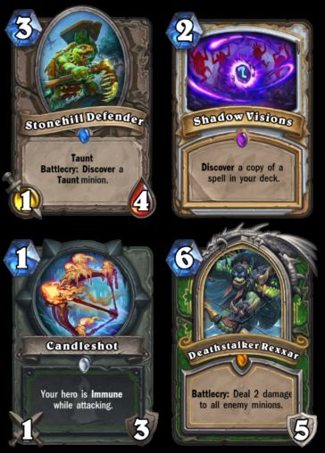
iii

STATEMENT OF AUTHORSHIP

 Thesis:

 Name: Tony                  Surname: Schwensfeier

 Date of Birth: 21.09.1993   Matriculation no.: 200068

I herewith assure that I wrote the present thesis independently, that the thesis has not
been partially or fully submitted as graded academic work and that I have used no
other means than the ones indicated. I have indicated all parts of the work in which
sources are used according to their wording or to their meaning.

I am aware of the fact that violations of copyright can lead to injunctive relief and
claims for damages of the author as well as a penalty by the law enforcement agency.

Magdeburg, 11.03.2019

Signature
v

                                   Abstract
              Prediction of Player Moves in Collectible Card Games

The prediction of moves of opposing players in a game is a task of each CI which
wants to call itself intelligent. In Collectible Card Games (CCG), this challenge is
complicated by a great number of strategies, or decks, and, therefore, the great
set of moves, or cards, the opponent can choose from. So how can a CI method
be accomplished, which maximizes the number of correct card predictions in a
CCG? During this thesis, a CI method was developed which can predict cards and
decks based on a data set of recently played decks. These decks defined the present
metagame of the game ’Hearthstone’. Card were predicted by stochastic calculations
on the hierarchically clustered decks. In the process, different distance functions and
linkage methods for the hierarchical clustering were evaluated. A 90% correct card
prediction on card sequences of decks exclusively from the metagame and a 40%
correct card prediction on card sequences of decks evolving from the metagame were
achieved which was an increase of 20% in contrast to the purely stochastic based
prediction method.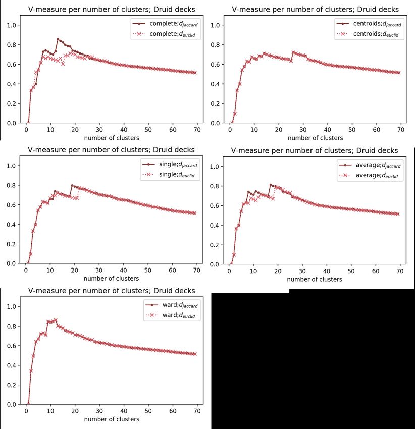
vii

                        Acknowledgements
At this place, I want to acknowledge my examiner Prof. Dr. habil Rudolf Kruse and
my supervisor Alexander Dockhorn who made possible to work at this thesis. I want
to thank my supervisor for the time that he offered when I had problems or needed
advice, and especially for his guidance in plotting data which I gained during my
evaluation.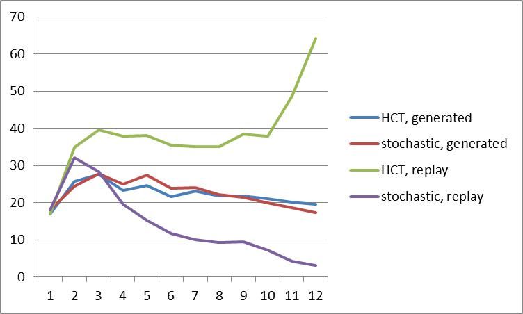

ix

Contents

STATEMENT OF AUTHORSHIP                                                                      iii

Abstract                                                                                      v

Acknowledgements                                                                             vii

1   Introduction                                                                              1
    1.1   Games . . . . . . . . . . . . . . . . . . . . . . . . . . . . . . . . . . . . .     2
          1.1.1   What is a Game? . . . . . . . . . . . . . . . . . . . . . . . . . . .       2
          1.1.2   Card Games . . . . . . . . . . . . . . . . . . . . . . . . . . . . . .      3
          1.1.3   Collectible Card Games . . . . . . . . . . . . . . . . . . . . . . .        4
          1.1.4   Hearthstone . . . . . . . . . . . . . . . . . . . . . . . . . . . . . .     4
    1.2   Research Questions . . . . . . . . . . . . . . . . . . . . . . . . . . . . . .      6
    1.3   Structure of this thesis . . . . . . . . . . . . . . . . . . . . . . . . . . . .    7

2   Background                                                                                9
    2.1   Game Theory . . . . . . . . . . . . . . . . . . . . . . . . . . . . . . . . .       9
    2.2   Machine Learning . . . . . . . . . . . . . . . . . . . . . . . . . . . . . . . 11
          2.2.1   Supervised Learning . . . . . . . . . . . . . . . . . . . . . . . . . 11
          2.2.2   Unsupervised Learning - Clustering . . . . . . . . . . . . . . . . 12
                  2.2.2.1   k-means clustering . . . . . . . . . . . . . . . . . . . . . 12
                  2.2.2.2   Hierarchical clustering . . . . . . . . . . . . . . . . . . 14
                  2.2.2.3   DBSCAN . . . . . . . . . . . . . . . . . . . . . . . . . . 15
    2.3   Stochastic . . . . . . . . . . . . . . . . . . . . . . . . . . . . . . . . . . . . 17
          2.3.1   Permutation . . . . . . . . . . . . . . . . . . . . . . . . . . . . . . 17
          2.3.2   Variation . . . . . . . . . . . . . . . . . . . . . . . . . . . . . . . . 18
          2.3.3   Combination . . . . . . . . . . . . . . . . . . . . . . . . . . . . . 19
          2.3.4   Experiments and events . . . . . . . . . . . . . . . . . . . . . . . 20
          2.3.5   Probability . . . . . . . . . . . . . . . . . . . . . . . . . . . . . . . 21
    2.4   Multisets . . . . . . . . . . . . . . . . . . . . . . . . . . . . . . . . . . . . 21
    2.5   Related work . . . . . . . . . . . . . . . . . . . . . . . . . . . . . . . . . . 22
          2.5.1   Evaluation of Hearthstone game states with neural networks
                  and sparse auto encoding . . . . . . . . . . . . . . . . . . . . . . 23
          2.5.2   Hearthstone: Finding the optimal play . . . . . . . . . . . . . . 23
          2.5.3   I am a legend: hacking Hearthstone using statistical learning
                  methods . . . . . . . . . . . . . . . . . . . . . . . . . . . . . . . . 24
x
3 Implementation 25
3.1 Playing Collectible Card Games . . . . . . . . . . . . . . . . . . . . . . . 25
3.1.1 Classification by game theory . . . . . . . . . . . . . . . . . . . . 25
3.1.2 Building a strategy . . . . . . . . . . . . . . . . . . . . . . . . . . 27
3.2 Selection of a test environment . . . . . . . . . . . . . . . . . . . . . . . 29
3.3 Stochastic conditions and problems . . . . . . . . . . . . . . . . . . . . . 32
3.4 Clustering of the meta data . . . . . . . . . . . . . . . . . . . . . . . . . 35
3.5 Search in a hierarchical cluster tree . . . . . . . . . . . . . . . . . . . . . 37
3.5.1 Restructuring the data . . . . . . . . . . . . . . . . . . . . . . . . 38
3.5.2 Traversing the HCT . . . . . . . . . . . . . . . . . . . . . . . . . 38
3.5.3 Calculate card, deck and win probabilities . . . . . . . . . . . . 39
3.6 Predictions . . . . . . . . . . . . . . . . . . . . . . . . . . . . . . . . . . . 40
4 Evaluation 41
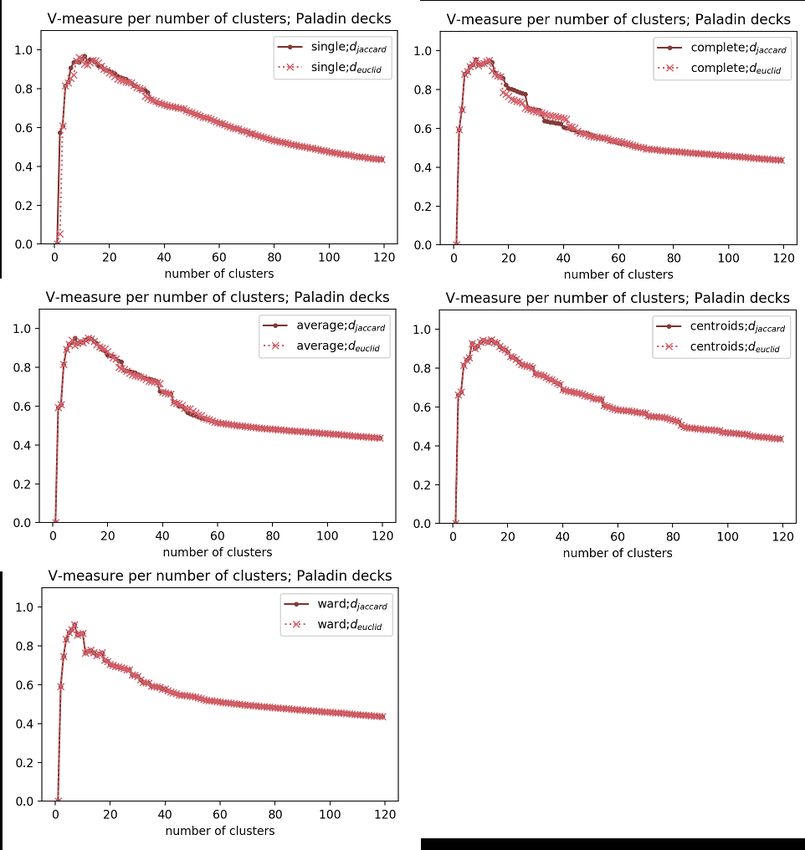
4.1 Clustering evaluation . . . . . . . . . . . . . . . . . . . . . . . . . . . . . 41
4.1.1 Criteria for the test data selection . . . . . . . . . . . . . . . . . . 41
4.1.2 Clustering the Data . . . . . . . . . . . . . . . . . . . . . . . . . . 42
4.1.3 Cluster validation . . . . . . . . . . . . . . . . . . . . . . . . . . . 43
4.1.4 Discussion . . . . . . . . . . . . . . . . . . . . . . . . . . . . . . . 46
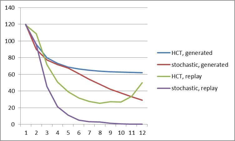
4.2 Prediction analysis . . . . . . . . . . . . . . . . . . . . . . . . . . . . . . 46
4.2.1 Prediction test data . . . . . . . . . . . . . . . . . . . . . . . . . . 46
4.2.2 Card Prediction . . . . . . . . . . . . . . . . . . . . . . . . . . . . 48
4.2.3 Card Prediction Validation . . . . . . . . . . . . . . . . . . . . . 49
4.2.4 Discussion . . . . . . . . . . . . . . . . . . . . . . . . . . . . . . . 50
5 Conclusion 53
A Distance Matrices 63
B Dendrograms 65
C V-measure 67
D Success Rate of Card Predictions 69
Bibliography 711 Chapter 1 Introduction Enthusiasm for Computational Intelligence (CI) is part of human history since the early days of the first automatons. This enthusiasm was routed in the wish to understand human nature and to improve the life through this new knowledge. The earliest ideas of realizing Computational Intelligence were automatons. After the first attempts of developing such machines were exposed as a swindle, where people controlling the machine from the inside, genuinely autonomous automatons were created. Examples are the writing and drawing automatons of the father and his son Jaquet-Droz around 1770. Multiple decades, their machines could be visited as they traveled through Europe.[1] With the early understanding of the human brain through the newly established science of neurology in the years of 1930 and 1940, approaches to realize an Artificial Intelligence (AI) were developed. Important foundations were made by Alan Turing’s theory of computation which defined the theoretical functionality of a computer, based on ’0’ and ’1’. Furthermore, it was possible with his work to design the Turing test which claimed that the consideration of a machine as ’intelligent’ is linked to the missing distinguishability of its response as human or mechanical.[2][3] The invention of the computer as we know in the years of 1950 and its predecessors inspired people to the development of AI. The first official founding of this discipline was in 1956. In the center were the game checkers. Nevertheless, the agents, AI-based software programs, in these games were not able to challenge the best players for a long time. They were based on simple brute-force techniques which, despite their simplicity, created good results. As a consequence, most of the research focused on the improvement of brute-force performance in developing faster data structures and search algorithms. In the following decades, many significant breakthroughs were made. The first one was the improvement of the computational processing power and the second one was the development of new techniques, based on the realization that brute-force can not be improved further. To that time, after many iterations, IBM’s agent Deep Blue was able to defeat the world champion in chess in 1996. [4] Furthermore, the term ’Computational Intelligence’ was introduced which used in this work instead of referencing to the term ’AI’. Why is CI still relevant? The usage of Computational Intelligence, as software
2                                                              Chapter 1. Introduction

on a home computer, robot or other devices has some significant advantages over
human work. CI does not get tired, has few needs, remembers more efficient and
works faster than humans. There are still areas, CI can not faultlessly be used or
can not be used at all, like government or emotional related work. They have still
problems to understand the new tasks, which they are not developed for. Yet there is
the opportunity that they will do the kind of work, a human can not do or are not
willing to do. I think that we should continue to develop CI further so that it can be
used in further areas. Recent developments highlight some interesting applications
for CI in society.
    First, In the industrialized nations, we stand in front of the problem of an aging
population. Robots can become our caretakers and companions. Examples are the
robot caretakers for lifting elders, Pepper the informational robot or Paro, the socially
assistive seal robot. [5, 6, 7]
    Second, the high signal transmission time between mars and earth up to 22.3
minutes makes it impossible to operate a Mars Rover from Earth in real time. Further-
more, it is currently not possible to send an operator to mars. So a software, named
AEGIS, is used to determine the next target of the latest Mars Rover, Curiosity. [8, 9]
    Third, a CI which is able to win against world champions in Chess, Shogi, and
Go, points out the potential from CI as opponents and teachers. So multiple shogi
players in Japan use teaching software to increase their skill. [10]

1.1     Games
Computational Intelligence finds multiple usages in games, in their development,
debugging and in the game as opponent or administrative system. Characteristics of
a game in general, particularly Trading Card Games, and the problems which they
create for CI, are covered in the following. Possible solutions are discovered by using
the game "Hearthstone" in this thesis later on. Basics of this game are explained in
this section.

1.1.1   What is a Game?

From the scientific point of view, a game follows a sequence of moves from a given
starting state. The state of a game is called game state. The moves translate the game
in from one game state into another. They are chosen by players among possibilities
or determined randomly by something like a dice roll or mixing cards. A different
amount of knowledge is offered to each player about the game, and when the game
ends or during the game, players get rewards. [11]
    So first, we distinguish based on the outcome of moves with regard to their
randomness:
1.1. Games 3
• In deterministic games, the outcome of a move is determined before it is made,
like chess, where the next position of a piece is determined by its current
position and the player’s move.
• In stochastic games, the outcome of moves is based on stochastic events. Game
examples are poker, roulette or Yahtzee, where the next game state is determined
by the stochastic result of shuffling cards, spinning a wheel or throwing dice.
A game can have deterministic elements as well as stochastic elements.
Second, we distinguish a game by the amount of available knowledge:
• With perfect information, each player has the complete knowledge of the state
of the game and every player has the same information. Examples are games
like chess or checkers, in which all pieces on the board are visible to all players
• With partial(imperfect) information, each player has the knowledge of a part
of the game state. Examples of such games are poker or bridge. In poker, the
revealed cards are visible to all players. Nevertheless, each player only knows
the cards of its hand and has no complete knowledge of the cards in the deck
and their order.
Third, a game is characterized by its reward. It is represented in the form of
ordinal data, win, draw and loose, or in the form of numerical data, as the number of
chips won in a poker game.
1.1.2 Card Games
Card Games are a prevalent type of games, and they generally have partial informa-
tion and the outcome is strongly dependent on stochastic events. These characteristics
have a fascinating influence on a working CI, which can not calculate the next possible
moves with the limited amount of information of the game state, so it has to guess
about the state.
Each card game consists of one or multiple decks. A deck is a set of cards, which,
in classic card games, depends on mostly unique cards with common themes. In
the case of French playing cards, there are four kinds of suits, numbered and faced
cards. Each Player gets a number of randomized cards before the game begins and/or
during the game, which are not known by the other players. Nevertheless, the players
know the deck and can guess the cards of their opponent by calculating based on
knowledge of their cards and the already played cards. They try to maximize their
reward over time while playing. Not knowing the cards of the opponent, yet knowing
the cards of the deck reduces the number of possible cards. Another type of card
games removes this knowledge base, replaces it with unique decks and thereby
creates an imperfect information game game with less information. Therefore, other
methods have to be used to guess the opponents’ cards. This type of card games is
described in the following.4 Chapter 1. Introduction
F IGURE 1.1: Logos of popular CCGs, from left to right: Hearth-
stone[15], MTG[12], Pokémon TCG[13], Yu-Gi-Oh![14], Shadow-
verse[16]
1.1.3 Collectible Card Games
In 1993 a new type of card game was released by the company ‘Wizards of the
Coast’[12]. It was a Collectible Card Game (CCG) called ‘Magic the Gathering’,
in short, ’MTG’. Later on, driven by the big financial success of the game, other
companies made their own game, popular examples are ‘Pokémon: Trading Card
Game’, in short, ’Pokémon TCG’[13], and ‘Yu-Gi-Oh!’[14]. The logos of some of the
current most popular CCGs are shown in Figure 1.1.
In CCG, each player creates its deck, based on deck-building rules, using a set
of cards, which were produced for this game. Players can purchase these cards by
buying booster packs, a packed set of randomized cards. The cards have different
types and, therefore, follow a different role in the game. As resource cards, they pay
for other card types, like creature cards, which can attack, or spell and object cards,
which can have multiple purposes. The players try to achieve a goal, which lies, in
most cases, in reducing the number of points of the opponent to zero or destroy a
certain number of creatures.
A good built deck is a good strategy and the key to win the game. However,
since cards are randomly distributed, they are hard to collect. Because of this reason,
players trade their cards with one another. In consequence, they can also be found by
the name ‘Trading Card Game’(TCG). Nowadays, the name is less applicable, because
of the recently developed online CCG, which do not allow this kind of interaction
between players anymore, yet offer another way to collect the needed cards.
1.1.4 Hearthstone
One of the most popular online CCGs is ‘Hearthstone: Heroes of Warcraft’[15], in
short, ’Hearthstone’, which was released in 2014 and developed by the company
’Blizzard Entertainment’. Its popularity created a big community which collects huge
amounts of information about the games. The active community created APIs which
results in the growing interest of scientists to use ’Hearthstone’ as a test platform
for their AIs. The following schematic overview of the game rules will be important
during this thesis. The more specific rule set can be accessed on Hearthstone Wiki page
[17]. For other related work to this subject, read more in 2.5.
In this CCG, a deck is built around one out of nine possible heroes, which represent
one player in a game. They have attributes like health, which can be reduced by
taking damage and can sometimes even attack the opponent. If the health of a
player’s hero reached zero the hero dies and the player loses the game. The health can1.1. Games 5
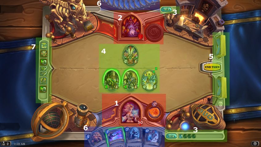
F IGURE 1.2: Example of a Hearthstone game board, 1. Player and its
Ability, 2. Opponent and its Ability(already used), 3. Mana, 4. Oppo-
nent’s minions (top row) and player’s minions on the board(bottom
row), 5. Decks, 6. Hand cards, 7. Play history
be protected by additional armor for the hero, who receives it through card effects.
Destroying the hero of the opponent is the goal of the game. Furthermore, heroes
have an ability, which can be activated once each turn. The game is separated in
alternating turns, where players draw a card from their deck, play cards and attack
with their creatures. They begin the game with zero Mana, which increases by one in
the player’s turn until it reaches a maximum of ten Mana. The deck of each player
contains 30 cards that the player can choose out of a set of over thousands of cards.
They are either free or restricted to one specific hero. The game format the deck is
played in is an additional restriction. Hearthstone provides two game formats.
• The Standard format is a balanced format, which permits cards of card sets of
the current or previous calendar year, as well as basic sets. Sets of new cards
are added to the game several times a year.
• The Wild format is unrestricted, i.e., every card released can be played in it.
Both formats can be played in ’Ranked’ and ’Casual Play Mode’, whereby the per-
formance of a player and the number of games played in the ’Ranked Play Mode’
defines the player’s ’Rank’ which ranges from the lowest rank fifty to the highest
rank zero.
The cards in Hearthstone have five grades of rarity, which is a measure to represent
their general strength. Free, common, rare and epic cards are allowed to be contained
twice in a deck, legendary cards are allowed once. There are four main card types.
They are shown in Figure 1.3.
• Minion cards are the creatures in Hearthstone. They can be played by paying
their Mana costs and are permanently in play until they are destroyed. They6 Chapter 1. Introduction
are positioned in a single line for each player which contains up to 7 minions.
Minions have an attack value and a health value. Minions can either attack
minions of the opponent or the opponent’s hero. When minions attack one
another, each takes the damage in the amount of the others attack value, which
decreases their health by this value. When it attacks a player, the player’s hero
health is decreased by this value. The health does not regenerate over time,
and a creature dies if its health value reaches zero. Minions can have triggered
abilities, which activates when played, when dying and other situations, or
passive abilities, such as preventing the opponent’s creatures in attacking the
player.
• Spell cards can be played by paying their Mana costs and leave the play after
their ability was processed.
• Weapon cards can be played by paying their Mana costs. They have an attack
value and durability value. They enable the hero of a player to attack minions
or the other player. By doing so, the hero does damage equal to the attack value
of the weapon. In return, the hero will receive damage in the amount of the
target’s attack value, and the durability of the weapon is reduced by one. A
weapon will be destroyed if its durability reaches zero or when a new weapon
is played.
• Hero cards can be played by paying their Mana costs. When played, they
replace the current hero and its ability. They keep the hero’s attack, yet add
armor to its health.
When cards interact with each other, it is called a synergy which might be stronger
than an ability by itself. Such as a minion card which regenerates the hero’s health
whenever a minion is played and a second minion card which damages the opponent
hero’s health whenever the own hero regenerates health. Cards can have a value for
the game, on their own or in synergy with other cards. So building a deck requires
specific knowledge of the cards. Deck building is a factor that influences the chances
of winning a matchup before the game started. Understanding the cards, the types
of deck they form, and the advantages of decks against others results in interaction
between the players. They choose promising decks and develop new types of decks
which might have new advantages. That creates a game in itself, which is called
metagame.
1.2 Research Questions
Problems which arise in playing CCG can be summarized as the following. Winning
the game requires (I) to optimize the own strategy and on further to (II) uncover
the strategy of the opponent player, so the moves of the opponent can be predicted
and countered. Both strategies influence the (III) chance of winning. Uncovering the1.3. Structure of this thesis 7
F IGURE 1.3: Example of the different card type, from top left to bottom
right: minion card, spell card, Weapon card, hero card[18]
opponent’s strategy is decisive influenced by the understanding of the metagame
which evolves by the creation of optimized strategies. That leads to the question.
How can a CI method be accomplished, which maximizes correct card predictions
using the metagame?
This research question can be specified by subdividing it into sub-questions which
this thesis tries to answer.
1. How can the metagame be represented?
2. Which information are derivable from the metagame?
3. What can be deduced from this information to predict cards?
1.3 Structure of this thesis
In the next chapter, the background knowledge is discussed which is build upon
to answer the questions, this thesis wants to answer. Related work shows related
problems and how they were solved.
Chapter 3 covers the problems which may occur and has to taken into account
when working with Hearthstone as a test environment and meta data. Different
solution strategies are discussed and proposed to cluster the meta data, and predict
the opponent’s deck and cards.
Multiple implementation variances for the clustering are considered and evalu-
ated in chapter 4. The card prediction algorithm is evaluated by its correct predictions.8 Chapter 1. Introduction
In the finishing chapter, the results are presented and interpreted. Various con-
cepts are suggested to extend the thesis and the use of the result in other areas than
Hearthstone and games.9
Chapter 2
Background
This chapter discusses some background, the thesis is build around. First, some
general topics on game playing in section 2.1 and machine learning in section 2.2
are considered. Next, basics of stochastic are in the focus in section 2.3 and (fuzzy)
multisets are explained in section 2.4, which this thesis is build up on. Finally, some
important previous work is summarized in section 2.5, that has been published on
Card Games, especially CCGs like ’Hearthstone’, and machine learning.
2.1 Game Theory
In this section, we will discuss the core concepts of Game Theory. Their influence on
CCG is discussed in section 3.1 later on. Game Theory is by K. Salen, E. Zimmermann
[11], and J. Schell [19].
In game theory, a game is distinguished by its characteristics. A game has a
combination of the following characteristics
Cooperativeness: In a cooperative game, players are able to make agreements, which
will have a positive outcome for both sides. On the other hand, a game is non-
cooperative, if players can not form alliances, this may be enforced by the game rules
itself or the decision of the players, or that the outcome of a game is not positive for
all players.
Symmetry: In a symmetric game the payoff is based on the strategies combination
and not the players. Exchanging the players’ results in the same payoffs. Table 2.1
shows the payoffs of a symmetric strategy and table 2.2 of an asymmetric strategy.
Zero-Sum: Is the Sum of the payoffs of all player for all strategy combinations equal
0, it is a zero-sum game. The strategies neither decrease nor increases the resources
of the game. Table 2.3 shows the payoffs of an zero-sum game and table 2.4 of a
non-zero-sum game.
A B
A 0, 0 -2, 1
B 1, -2 -2, -2
TABLE 2.1: symmetric strategy10 Chapter 2. Background
A B
A -2, -2 1, -2
B 1, -2 0, 0
TABLE 2.2: asymmetric strategy
A B
A 0, 0 -2, 2
B 2, -2 -4, 4
TABLE 2.3: zero-sum game
In context to the symmetry and zero-sum is the Nash equilibrium which describes a
situation in which two players keep their strategy, since the change of the strategy
results in a worse payoff for the changing player. The strategies A(row) and B(column)
of Table 2.3 shows such a situation.
Move-Order: The Move-Order can be one of these two. First, is the action-order
simultaneous, both players make their move at the same time or in the unawareness
of the other players’ previous move. Second, is the action-order sequential, players
know previous players’ actions.
Information: Perfect information games are a subset of sequential games, where
all players have complete information on all the other players’ previous moves, for
example, chess and Go. In most games, players have imperfect information(partial
information) of the game state, like Poker.
Game length: We can distinguish games by their length, the maximum number of
total possible game steps, in which players make their move. Some games consist
of only one game step, like Rock–paper–scissors. Other games have multiple or an
infinite number of game steps, which is the case for many single player or cooperative
multi-player video games.
Metagame: It is summarized in a video of Stanislav Costiuc [20] The metagame (’meta’
from Greek for ’about’, ’beyond’) is a literally ’a game beyond the game’. Depending
on the context, the word is used two describe two different things. The mechanical
metagame is a set of systems and mechanics which is wrapped around the gameplay
by the developer. The emergent metagame is strategies that transcend the rules and
systems of a game which emerging from the player interactions. This definition of
the metagame is used in game theory and which is used in this thesis further on.
The metagame occurs specifically in competitive games is strategies the players
utilize. Considering a Rock–paper–scissors game, the strategy of a player is not only
based on the payoffs of the current game, but also on the meta factors of the previous
game. If the opponent takes every time the move ’rock’ the move ’paper’ premises
a better payoff in the metagame. Though this scenario might be promising for the
current state of the metagame, it is not for the following games, since the metagame
is emergent. It means that the opponent will adjust his strategy to the metagame2.2. Machine Learning 11
A B
A -2, -2 1, -2
B 1, -2 0, 0
TABLE 2.4: non-zero-sum game
which results in a cycle of the metagame. The emerging of strategies is very specific
to CCGs. It can be divided into four phases:
1. In the experimentation phase, many strategies are tried out by the players. No
strategy is dominant, i.e., is played signally played more than others.
2. In the stabilization phase, effective strategies which have been found during
the experimentation become dominant. Strategies against strategies and moves
to defend the own strategy are found. It is a phase of balancing.
3. In the meta solved phase, all strategies are known, resulting in a few dominant
strategies and the payoff of a game becoming mainly a matter of player skills.
4. In the shake up phase, a new strong strategy is found, a balance is released
which changes the rules, or a new expansion with new rules and moves is
released, resulting in new experimentation or stabilization which length is
depended on the impact of the shake up.
2.2 Machine Learning
Machine Learning are AI Methods which focus on building a mathematical model of
sample data, also training data, for the purpose of making decisions or predictions
without being told to do so. Types of machine learning are supervised and semi-
supervised learning, unsupervised learning and reinforcement learning. Supervised
learning and especially unsupervised learning are covered in the Data Mining book
[21] and in the book by Togelius and Yannakakis [22] and explained in the following.
2.2.1 Supervised Learning
Supervised learning is a process to train a CI agent with labeled data to find char-
acteristics in the data the label can be identified with. To do so, it approximates the
underlying function between labeled data and their corresponding attributes and
features. For instance, to distinguish between knife and fork, an agent receives a set
of data to learn from, examples of cutlery, which contain the information about their
attributes, like form, size and material, and their corresponding labels (target output),
such as fork and knife. So it is supervised because the target output is known. After
learning is complete, the algorithm should be able to tell if new unseen cutlery is a
knife or fork by its attributes. The goal is, to learn from in-and-output pairs and to
create a mapping function which is able to work with new unseen instances of input12 Chapter 2. Background
data.[22] Three main types of supervised learning algorithms can be identified by the
data type of the labels:
Classification is an attempt to predict categorical class labels(discrete or nominal)
such as knives and forks.
With regression it is possible to predict intervals such as the length of a rain shower.
Preference learning teaches a CI to rank new data and to give ordinal output, such
as ranking a social media post by its obscenity or racism.
2.2.2 Unsupervised Learning - Clustering
Unsupervised Learning is a process to find and analyze similarities between data
input like supervised learning, except the learning data are not labeled. In other
words, the target output is unknown. The algorithm searches for patterns in the
input data attributes. The focus is on intrinsic structures of the input data and in their
associations instead of predicting target values.[22]
One subfield of unsupervised learning is clustering. The task of clustering is to
find groups (cluster) in a number of data points so that the attributes of each point
in a group are similar and dissimilar to attributes of other groups’ data points. It is
used for group detection in multidimensional data and reducing tasks, such as data
compression, noise smoothing, and outlier detection. Since the target clusters are
unknown, good clusters are characterized by high intra-cluster similarity, or high
compactness, and low inter-clusters similarity, or good separation. However, these
properties are no measure of a cluster’s meaningfulness.
Furthermore to the characteristics described above, cluster algorithms are defined
by their membership function and a search procedure. The membership function
defines the degree of assignment from the data samples to a cluster. The search
function describes the strategy of clustering the data using the membership function,
such as separating all data points into clusters at once as in k-means and DBSCAN,
or recursively as in hierarchical clustering. These three clustering procedures are
explained in the following.
2.2.2.1 k-means clustering
k-means is a partitional-clustering algorithm and a vector quantization method,
which is because of its good balance between simplicity and effectiveness considered
the most popular clustering algorithm. It follows a data partitioning approach of
partitioning data samples into k clusters, so that the sum of distances (or quantization
error) between data points and their corresponding cluster centers is minimized.[22]
A cluster is defined by its data points and its cluster center, which is the average
of all to the cluster assigned data points. Each data point is assigned to the cluster
with the smallest distance. The clustering algorithm requires multiple iterations of2.2. Machine Learning 13
alternating between calculation of the cluster center and reassigning of the data points
to the closest cluster center, begging with a randomized allocation of data points to
clusters which number is defined beforehand. The basic steps are the following:
Given k
1. Randomized partitioning of data points into k non-empty clusters
2. Calculation of the cluster centers
3. Assignment of each data point to the closest cluster center
4. Stop if each data point remains by it current cluster center, else continue with 2
Data points are objects which can be described as a vector. Depending on the
data set, it is beneficial to use different ways to calculate distances of two vectors
p = ( p1 , p2 , . . . , pn ) and q = (q1 , q2 , . . . , qn ). Three distance functions are:
• The Manhattan distance is sum of distances of two vectors p and q on each
axis.[23]
n
dis Manh ( p, q) = ∑ | pi − qi | (2.1)
i =1
• The Euclidean distance is the square root of the sum of squared distances of
two vectors p and q on each axis.[23]
s
n
dis Eucl ( p, q) = ∑ ( p i − q i )2 (2.2)
i =1
• If the data points are sets A, B which are not associated with a vector, the
Jaccard index offers a way to measure the similarity and diversity of the sets.
By its subtraction from 1, the Jaccard distance is calculated.[24]
| A B|
T
dis Jac ( A, B) = 1 − J ( A, B) = 1 − (2.3)
| A B|
S
Despite its effectiveness, k-means has some disadvantages and is not applicable
in some situations. First, data objects have to be in continuous space. Second, it
only finds convex clusters what results in favoring hyper-spherical clusters. Third,
the number of clusters k has to be specified in advance. Finally, k-means is weak
against outliers, data points with extremely high distances to others, since they may
distort the distribution of data and may influence the performance of the algorithm.
Hierarchical clustering is a different approach of clustering which fixed some of these
issues and is described in the next paragraph.14 Chapter 2. Background
2.2.2.2 Hierarchical clustering
Hierarchical clustering is a clustering method which attempts to build a hierarchy
of clusters. Two methods exist to build a hierarchy. The agglomerative strategy is
an bottom-up method which gradually merges clusters together until a termination
criteria is met or one single cluster is left. In contrast, the divisive strategy creates
cluster hierarchies by splitting up clusters top-down until every data point is in its
own cluster, starting with a single cluster which contains all data points. Both using
distance matrices as cluster strategy.[22]
basic steps of an agglomerative clustering algorithm is presented in the following:
Given k
1. Creation of one cluster for each data point
2. Creation of the distance between, containing the distance of all clusters
3. Finding and merging of the closest clusters
4. Stop if there are k clusters; otherwise continue with step 2
The distance between is represented by a distance matrix. The calculation of the
distances matrix, and the merging of clusters requires linkage methods which use
distance functions, such as Euclidean or Manhatten distance. The following linkage
methods can be distinguished:
• single linkage: This method searches for the closest points between two clus-
ters(or inter-cluster distance), their distance is the cluster distance. Once the
distance between all clusters are calculated. The clusters with the smallest
distance are merged. The feature of single linkage is, that it leads to chains in
the data.[25]
• complete linkage: In contradiction to single linkage, this method tries to find
the biggest inter-cluster distance, i.e. the farthest points between to clusters,
their distance is the cluster distance. As in single linkage the closest clusters are
merged. Complete linkage and the following methods tend to create circular
clusters.[25]
• average linkage: The cluster distance in this method is the average over all
pairwise distances between all data points between two clusters. As before,
clusters with the closest distance are merged.[25]
• centroids: In contrast to average linkage, this methods calculates the average
of all data points and creates a centroid for each cluster before measuring the
distance. The clusters with the closest distance of their centroids are merged.[25]
• ward’s minimum variance method: Similarly to centroids, centroids are cre-
ated of each cluster. Next, a centroid for a simulated merge of both clusters
is created. The distances of data points to their centroid are compered to the2.2. Machine Learning 15
F IGURE 2.1: Dendrogram plot example [27]
distance of them to the simulated centroid of both clusters. Clusters with the
smallest deviation are merged. [26]
Once all cluster steps (merging or splitting) are completed, each step of the
algorithm can be visualized in a tree representation. With the cluster which contains
all data points as root, each merging clusters as children merged clusters as their
parent and one-elemental cluster in the lowest layer. The edges of this, so-called
dendrogram, are weighted with the merging (or splitting) costs, in this case, the
cluster distance. The final cluster is created by cutting the dendrogram at the desired
level of merging costs. A plot example of a dendrogram can be seen in Figure 2.1.
Hierarchical clustering is greedy, meaning that it merges local optima, which may
not result in the global optimum.
2.2.2.3 DBSCAN
In focus of density based clustering is the concept of finding dense regions of data
points with low density space (noise) between them. The main representative of
density based clustering is DBSCAN. It detects clusters by the high density of data
points inside the cluster and low density outside of it. The clustering process is
incremental.[21]
DBSCAN is based on the two concepts of density reachability and density con-
nectivity. Both build upon two input variables, the size of the epsilon neighborhood
(e) and the minimum points in range (m). DBSCAN has the key idea that, for each
point of a cluster, at least m other points are in the neighborhood of range e.
Density reachability ask for the question, whether two points are in the same
cluster. A point p1 is direct density reachable from p2 if the distance of p1 and p2 is
less than e, and at least m points are in e-neighborhood of p2 . A point pn is density
reachable from a point p0 if a sequence of points between them exists whose points are16 Chapter 2. Background
direct density reachable from the previous one beginning by p0 . Density connectivity
is the build-up step of DBSCAN. If two points p1 and p2 are density reachable from a
third point p0 , p1 and p2 are density connected.
DBSCAN classifies points into point type which are core points, border points and
noise points. core points have at least m points in their e-neighborhood. boarder points
are in range of a core point, though, have fewer than m points in their e-neighborhood.
noise point is any that that is not core point or boarder point. The following steps are the
main ones of DBSCAN.
1. Selection of a starting point p
2. Retrieval of the point in e-neighborhood of p and classification into point type
3. If the point is a core point, creation of a new cluster or extension of exiting cluster
or merging of clusters if p is density reachable from points in e-neighborhood
and points are in different clusters
4. Stop if all points have been processed; else continue with step 2 with the next
point in the database
Advantages of DBSCAN include that the number of clusters is not required
apriori. Furthermore, it is able to find find arbitrarily shaped clusters and can detect
outliers. Since the variable m is selected globally, it may have problems clusters of
different densities, though, solutions approaches are existing. Since the algorithm
process uses distance operations, it may find the curse of dimensionality problem for
high-dimensional data sets.2.3. Stochastic 17
Did the selection of elements
already take place?
s no
ye
Are all elements Is the order of
distinct? the selection relevant?
s
s
no
no
ye
ye
permutation permutation with returning with returning
without repetition with repetition of elements? of elements?
yes
yes
no
no
variation variation combination combination
with without with without
repetition repetition repetition repetition
F IGURE 2.2: Differentiation of permutation, variation and combination
with and without repetition
2.3 Stochastic
Stochastic is a sub-field of mathematics which is subdivided into probability theory
and mathematical statistics. It is about the number of events, their possible outcome,
and their probability and is discussed by H. Rinne [28], and D. Maintrup and S.
Schäffler [29].
The combinatorial analysis is part of probability theory. Its focus is the consid-
eration of the number of element combinations. The combinatorial analysis can be
distributed into three different subfields, which are the permutation, the variation,
and the repetition. The distribution is determined by the selection of the elements,
the differentiation of the elements, the relevance of the order of the elements and the
return of the elements as shown in Figure 2.2.
2.3.1 Permutation
Permutation describes an arrangement of elements. All elements of a set are consid-
ered. They may occur once or multiple times. If all element are distinct, i.e. each
element occurs once, the permutation is a permutation without repetition. It is de-
fined that each unambiguous image Φn of an ordered set {1, 2, ..., n} on a set A of
size n is a permutation without repetition. P(n) is the number of permutations of n
distinct elements.
P(n) = 1 · 2 · ... · (n − 1) · n =: n! (2.4)18 Chapter 2. Background
F IGURE 2.3: permutation without repetition(left) and permutation
with repetition(right)
If at least an element cannot be distinguished from another one, i.e., it occurs
multiple times, the permutation is a permutation with repetition. Then, the matching
elements can be switched at their position in the distribution without changing the ar-
rangement of elements. It is resulting in a reduction in the number of possible arrange-
ments. For a permutation with repetition, it applies that when A = { a1 , a2 , . . . , ak }
is a set of k elements and n1 , n2 , ..., nk in N0 with ∑ik=1 ni = n. Each ordered n-tuple,
which contains the element a j exact n j times (1 ≤ j ≤ k ), is a permutation with repeti-
tion. Then, P(n|n1 , n2 , ..., nk ) is the number of permutations of n elements, where k
are distinct.
n! n
P(n|n1 , n2 , ..., nk ) = =: (2.5)
n1 ! · n2 ! · ... · nk ! n1 , n2 , ..., nk
with ∑ik=1 ni = n and 0 ≤ n j ≤ n∀ j.
(n1 ,n2n,...,nk ) is called the polynomial coefficient.
Figure 2.3 shows an example of a permutation with repetition and one without
repetition.
2.3.2 Variation
A variation is an ordered sample of elements of a set, i.e. it is an arrangement which,
in contrast to the permutation, does not compulsorily contain all elements of the
set. If the ordered sample contains all elements of the set, it is a permutation. As
in a permutation, the elements can appear once or multiple times. For a variation
without repetition, it is defined, that each ordered n-tuple of distinct elements of a
set A with the size N is a variation without repetition of N elements of the scope n,
with n ≤ N. A variation without repetition is a sample without returning of elements
of scope n from a set of N elements, where the order of the elements is important.
Since one element is selected and then removed from the set of remaining selectable
elements, the number of elements for the next selection is reduced by one. V ( N, n) it
the number of distinct variations without repetition.2.3. Stochastic 19
F IGURE 2.4: variation without repetition(left) and variation with repe-
tition(right)
N! P( N )
V ( N, n) = = (2.6)
( N − n)! P( N − n)
In contrast to a permutation, the occurrence of multiple elements in a variation,
i.e., the repetition, is created through selection from and returning of elements into the
selection pool, instead of the multiple existences of the same element. Each ordered
n-tuple of elements of a set A with size N is a variation with repetition of N elements
of scope n, with n ≤ N or n > N. A variation with repetition is a sample with
returning of elements of scope n from a set of N elements, where the order of the
elements is important. Since elements are returned into the scope after the selection,
the number of elements in the arrangement can extend the number of elements in the
set. The Number V ∗ ( N, n) of distinct variations without repetition is
V ∗ ( N, n) = N n (2.7)
Figure 2.4 shows an example of a variation with repetition and one without
repetition.
2.3.3 Combination
A combination is an unordered sample of elements of a set, i.e., it is an arrangement
which, as in a variation, does not compulsorily contain all elements of the set, and in
contrast to it, does not consider the order of elements. It is resulting in a reduction
of the number of possible arrangements, in contrast to the variation. Elements can
be selected once or multiple times. Each subset of size n from a set A of size N is a
combination without repetition of N elements of scope n, with n ≤ N. A combination
without repetition is a sample without returning of elements, where the order of the
elements is unimportant. C ( N, n) is the number of distinct combinations without
repetition which is calculated by the binomial coefficient ( Nn ).
V ( N, n) N! N
C( N, n) = = =: (2.8)
P(n) (n!( N − n)! n20 Chapter 2. Background
F IGURE 2.5: combination without repetition(left) and combination
with repetition(right)
The combination of all variations of N Elements with scope n with returning of
elements, which contain the same elements in an equal number, in an equivalence
class is a combination with repetition. A combination with repetition is a sample
with returning of elements, where the order of elements is unimportant. The number
C ∗ ( N, n) of distinct combinations with repetition is
N+n−1
∗
C ( N, n) = (2.9)
n
Figure 2.5 shows an example of a combination with repetition and one without
repetition. It is visualized that two samples in different order of elements are the
same, since the order is unimportant.
2.3.4 Experiments and events
An experiment is a repeatable process with an uncertain result under approximately
equal conditions, such as throwing dice. One possible result is called its outcome ωi
with i = 1, 2, . . . , N and the sample space Ω is the set of all distinguish outcomes. In
case of six-sided dice, the sample space contains the eye numbers one to six.
An event is a subset of outcomes of an experiment, such as the eye numbers
one to three. A certain event, i.e., an event that must occur, are the eye numbers
one to six since it is equal the sample space. A random event A, B, C, . . . is a strict
subset of (omega) and can be the eye numbers one and two. The elemental event is
a one-elemental random event, such as the eye number one.
For the throwing of a four sided dice, the events are as followed.
• elemental events: {1}, {2}, {3}, {4}
• other random events: {1, 2}, {1, 3}, {1, 4}, {2, 3}, {2, 4}, {3, 4},
{1, 2, 3}, {1, 2, 4}, {1, 3, 4}, {2, 3, 4}
• certain event: {1, 2, 3, 4}2.4. Multisets 21
2.3.5 Probability
The probability can be categorized definitely. In this work, it is defined in the prior
and objective way. The probability of an event Pr ( A) is indicated by the quotient of
the size of an event N ( A), i.e., the number of outcomes of an event, and the size of
the sample space N, i.e., the number of all possible outcomes.
N ( A)
Pr ( A) = (2.10)
N
The conditional probability of A given B P(A|B), given the two events A and B,
is defined as:
Pr ( A ∩ B)
Pr ( A| B) = (2.11)
Pr ( B)
Pr ( A ∩ B) is the probability that events A and B occur at the same time. A ∩ B
is called Intersection. In case of a sample space of men and women with different
ages, an intersection would be the selection of a 40 years old man. The event A and
B are stochastically independent, if Pr ( A ∩ B) = Pr ( A) · Pr ( B). According to the
multiplicity theorem, the intersection of multiple events is calculated as follows.
Pr (∩in=1 Ai ) = Pr ( A1 ) Pr ( A2 | A1 ) Pr ( A3 | A1 ∩ A2 ) . . . Pr ( An | A1 ∩ A2 ∩ . . . An−1 )
(2.12)
2.4 Multisets
The notation of multisets are discussed by S. Miyamoto [30], extracted from the work
of D. E. Knut [31]. Multisets are sets which can contain multiple instances of an
element. A crisp mulitset M is defined as
M = {k1 /x1 , . . . , k n /xn } (2.13)
over the the basic set X = { x1 , . . . , xn } with k i = γ M ( x1 ) the number of appear-
ances, or count, of xi in M.
Assume a basic set of elements X = { x, y, z, w}. For example two objects
with the label x, one object with the label y, zero objects with the label z, and
three objects with the label w are the multiset { x, x, y, w, w, w}. It can also be writ-
ten as {2/x, 1/y, 0/z, 3/w} to show the number for each element of the set X, or
{2/x, 1/y, 3/w} by ignoring elements which are not appear. In the example we have
γ M ( x ) = 2, γ M (y) = 1, γ M (z) = 0, γ M (w) = 3
The following are the basic relations and operations for crisp multisets. (inclusion):
M ⊆ N ⇔ γ M ( x ) ≤ γ N ( x ), ∀ x ∈ X. (2.14)22 Chapter 2. Background
(equality):
M = N ⇔ γ M ( x ) = γ N ( x ), ∀ x ∈ X. (2.15)
(union):
γ M∪ N ( x ) = max {γ M ( x ), γ N ( x )} = γ M ( x ) ∨ γ N ( x ) (2.16)
(intersection):
γ M∩ N ( x ) = min{γ M ( x ), γ N ( x )} = γ M ( x ) ∧ γ N ( x ) (2.17)
(addition):
γ M⊕ N ( x ) = γ M ( x ) + γ N ( x ) (2.18)
(subtraction):
γM N (x) = 0 ∨ γM (x) − γN (x) (2.19)
The symbols ∨ and ∧ are the infix notation of max and min. Consider N = 1/x, 2/z, 2/w
and the first example of M, Then,
M ∪ N = 2/x, 1/y, 2/z, 3/w
M ∩ N = 1/x, 2/w
M ⊕ N = 3x, 1/y, 2/z, 5/w
M N = 1/x, 1/y, 1/w
Furthermore, an extension of multisets, fuzzy multisets, are featured by S. Miyamoto
which where firstly discussed by R. R. YAGER [32]. While a fuzzy extension is not
further discussed here, it was discussed in a recently submitted paper, which builds
up on the work of this thesis [33].
2.5 Related work
Previous work to the game Hearthstone show implementation approaches of CI in the
game. A central element is the evaluation of game states as discussed in Subsection
2.5.1. From the current game state, a simulation is started to evaluate possible moves
by their payoff, though, future game states which are required for the simulation
are uncertain. A simulation based on card prediction and game state evaluation
is discussed as in Subsection 2.5.2. The approaches can deliver good results as the
prediction of cards with bigrams as discussed in Subsections 2.5.3, though, often
ignore decency of cards from their decks and predict by the decency of card to card.
A deck prediction can improve the existing approaches.2.5. Related work 23
2.5.1 Evaluation of Hearthstone game states with neural networks and
sparse auto encoding
The article of Jan Jakubik [34] describes an approach of evaluating game states in
the game Hearthstone. Goal was the evaluation of game states by machine learning
algorithm by usage of 2.5 million game state out of training samples of Monte Carlo
search tree driven agents. Sparse auto encoding was used to encode the information
of the Minions in play on the players side and the opponents side. These two vectors
and vectors which describe the turn number, the player’s stats, the opponent’s stats,
and the player’s hand were representing the game state. A five layer deep neural
network was trained with the training data to evaluate the game state and predict the
game’s result which was the output of a single output neuron.
The agent achieved the 5th place of the AAIA’17 data mining challenge out of 188
submissions. Main weakness was the insufficient representation of complex cards, i.e.
cards with unique effects.
2.5.2 Hearthstone: Finding the optimal play
The thesis of Tom Drijvers [35] describes an approach of evaluating game states and
guessing the opponents hand in the game Hearthstone. The aim was the development
of an decision supporting system for the player.
The goal of the evaluation was the scoring of the game state like a human player
would do. It was devided into five parts. Its parts were the health score for the players’
health and armor, the secret score for secret spells on the board, the hand score for
the number of cards in the players’ hands, the deck score for the number of cards
in the players’ decks, and the board score for the number and kind of Minions on
the board. They were combined by a weighted sum which was weighted based on
the players’ strategies by the player during the game or by the algorithm based on
previously defined weights.
The hand prediction was realized by a fuzzy set which represented the possibility
of cards in the opponent’s hand. During start of the game each hard had the same
degree of membership including cards which were not actually in the deck if the deck
was unknown. The fuzzy set was updated after the mulligan face which is motivated
by the assumption that a player will keep specific cards in their hand, e.g. cheap
cards or cards with high impact on the game state during the first turns of the game.
The next updates were done during the drawing of cards.
It was simulated in two steps. First, the playing of cards was tested. Second,
possible attackers were simulated. Both step were evaluated by the their change of
the game state. The CI was tested for player support and in fully automated mode.
Opponents were the CI itself and other CI. The weighting and hand predictions
were adapted during the tests. In the results, the CI preformed better than related
algorithms in the play and the evaluation had an advantage over standard evaluation
after the adaption.24 Chapter 2. Background
The CI was not tested against actual players, like the hand prediction was build
upon. The prediction of the opponent’s deck was not considered, though, the op-
ponent’s deck was adapted after knowing it. The simulations was not made over
multiple turns.
2.5.3 I am a legend: hacking Hearthstone using statistical learning meth-
ods
The CI of E. Bursztein [36] which uses Hearthstone card sequences to predict fu-
ture cards was called ’game breaking’ of the Hearthstone developer Blizzard. Its
prediction is based on learning from game-replays which cards are played signifi-
cantly more often then other cards and which cards are often played together. The
data were extracted from debug logs [37] and used to generate replays. Bigrams
were constructed on the sequence of played cards from the replays containing all
combinations of cards, and used to construct a co-occurrence table conting all this
co-occurrences happen. An ranked list of cards which are in the opponents deck
and likely to be played was created for the prediction, while summing the frequency
of card appearances of all retrieved cards that were co-played with the seen cards.
Burzstein evaluated the algorithm by generating the ranked list and comparing them
with the effectively played cards of future turns. Card prediction were mostly correct
up to 95% in the turns three to five. The dependence of a card occurence to a complete
deck was not considered.25 Chapter 3 Implementation CCGs are games, where information are hidden to an extent, though rules of the game and possible moves of a player are well known. Winning in a CCG requires the understanding of games and their theory, in general, to determine which type of game they are and how to classify them into game theory, so it is possible to develop a successful strategy. These topics are covered in section 3.1. The selection of a test environment has an influence on the agent who is playing the CCG. So a CCG game has to be chosen before its development. Factors for the selection of a CCG, test environment candidates, and the final choice are covered in section 3.2. After the selection of a CCG, an algorithm, which is part of the game playing agent, has to be build which tries to predict the opponent’s strategy in a whole and detect risks of moves which are part of the strategy. These risks are the cards of the deck which is the opponent’s strategy. Furthermore, if maximizing the number of total won is the goal of the agent, the will have to predict changes of winning a game, so the agent can decide whether to continue the game, if win chances are high or to end it if a loss is likely. Since stochastic conditions determine the cards of the opponent and its strategy, in combination with the metagame, they and the resulting problem are covered in section 3.3. Clustering of the metagame data which is the solution to this problem is the topic of section 3.4. The impacts on the stochastic conditions and the search on the Hierarchical Cluster Tree which was developed in the process are continued in section 3.5. 3.1 Playing Collectible Card Games Collectible Card Games are a subgroup of card games with special characteristics that distinguishes them from other card games, described in Subsection 1.1.3. Their classi- fication by game theory and the influence of their characteristics onto the strategies of playing the game are dealt with in the this section. 3.1.1 Classification by game theory Game Theory is a scientific field which deals with the strategies or player actions and the rules in a game. The basics of game theory are discussed in 2.1. CCGs can be
You can also read