Algorithm Theoretical Baseline Document for Sentinel-5 Precursor Methane Retrieval
←
→
Page content transcription
If your browser does not render page correctly, please read the page content below
Algorithm Theoretical Baseline
Document for Sentinel-5
Precursor Methane Retrieval

Otto Hasekamp, Alba Lorente, Haili Hu, Andre Butz, Joost

aan de Brugh, Jochen Landgraf

document number : SRON-S5P-LEV2-RP-001
CI identification   : CI-7430-ATBD
issue               : 1.10
date                : 2019-02-01
status              : released
S5P ATBD draft                                                SRON-S5P-LEV2-RP-001
issue 1.10, 2019-02-01 – released                                       Page 2 of 67

Document approval record
                  digital signature

 prepared:

                   Michael Buchwitz and Thomas Krings
 checked:          Institute of Environmental Physics (IUP)
                   University Bremen, Germany

 approved PM:

 approved PI:
S5P ATBD draft                                                                     SRON-S5P-LEV2-RP-001
issue 1.10, 2019-02-01 – released                                                            Page 3 of 67

Document change record
 issue     date          item               comments
 0.00.01   2012-09-25    all                Darft ATBD
 0.00.02   2012-11-08                       Comments internal review addressed. Note on the depend-
                                            ence of computational performance on compiler included.
                                            For GNU compiler significantly more processors are needed
                                            (60-90) than earlier estimated for the Intel compiler (page
                                            22).
 0.00.02   2012-11-23    doc number         Changed to report (RP) with new doc number
 0.05      2013-06-04    all                Several additions from draft to version 1: More extended
                                            algorithm description, extended sensitivity study, section on
                                            validation.
 0.05      2013-06-20    contents + doc     Addressed comments internal review, changed to new docu-
                         number             ment numbering
 0.09      2013-11-27    all                addressed reviewer comments
 0.10.00   2014-04-11    all                Removed instrument section. Introduced cirrus filter based
                                            on SWIR band. Slightly modified test ensemble to repres-
                                            ent more realistic AOT (more demanding than previous en-
                                            semble).
 0.11.00   2014-07-23    all                added fluorescence, deconvolution of solar spectrum, up-
                                            dated input/output tables, checked fraction of clear pixels
                                            with RAL VIIRS processor
 0.13.00   2015-08-31    table 5-3 and 6-   Update for limited release to S5p Validation Team; Made
                         1                  consistent with actual product
 0.14.00   2015-12-11    section 9          Improved quality of Fig 9-17
 1.00      2016-02-05    all                V1.0 release; Adressed comments from internal review (all
                                            minor)
 1.10      2019-02-01    Sec. 5.6           description of bias correction added
           2019-02-01    Sec. 6.3           Tab. 5 updated
           2019-02-01    Sec. 6.4           SZA data filter updated
           2019-02-01    Sec. 6.5           TBC specified
           2019-02-01    Sec. 9             added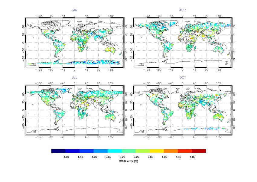
S5P ATBD draft                                                                                                                                                             SRON-S5P-LEV2-RP-001
issue 1.10, 2019-02-01 – released                                                                                                                                                    Page 4 of 67

Contents
Document approval record . . . . . . . . . . . . . . . . . . . . . . . . . . . . . . . . . . . . . . . . . . . . . . . . . . . . . . . . . . . . . . . . . . . . . . . . . . . . . . . .                              2
Document change record . . . . . . . . . . . . . . . . . . . . . . . . . . . . . . . . . . . . . . . . . . . . . . . . . . . . . . . . . . . . . . . . . . . . . . . . . . . . . . . . . .                            3
List of Tables . . . . . . . . . . . . . . . . . . . . . . . . . . . . . . . . . . . . . . . . . . . . . . . . . . . . . . . . . . . . . . . . . . . . . . . . . . . . . . . . . . . . . . . . . . . . . . . .        6
List of Figures . . . . . . . . . . . . . . . . . . . . . . . . . . . . . . . . . . . . . . . . . . . . . . . . . . . . . . . . . . . . . . . . . . . . . . . . . . . . . . . . . . . . . . . . . . . . . . .          7
1                   Introduction . . . . . . . . . . . . . . . . . . . . . . . . . . . . . . . . . . . . . . . . . . . . . . . . . . . . . . . . . . . . . . . . . . . . . . . . . . . . . . . . . . . . . .          9
1.1                 Identification . . . . . . . . . . . . . . . . . . . . . . . . . . . . . . . . . . . . . . . . . . . . . . . . . . . . . . . . . . . . . . . . . . . . . . . . . . . . . . . . . . . . . . .      9
1.2                 Purpose and objectives . . . . . . . . . . . . . . . . . . . . . . . . . . . . . . . . . . . . . . . . . . . . . . . . . . . . . . . . . . . . . . . . . . . . . . . . . . .                      9
1.3                 Document overview . . . . . . . . . . . . . . . . . . . . . . . . . . . . . . . . . . . . . . . . . . . . . . . . . . . . . . . . . . . . . . . . . . . . . . . . . . . . . . .                   9
2                   Applicable and reference documents . . . . . . . . . . . . . . . . . . . . . . . . . . . . . . . . . . . . . . . . . . . . . . . . . . . . . . . . .                                              10
2.1                 Applicable documents . . . . . . . . . . . . . . . . . . . . . . . . . . . . . . . . . . . . . . . . . . . . . . . . . . . . . . . . . . . . . . . . . . . . . . . . . . . .                      10
2.2                 Standard documents . . . . . . . . . . . . . . . . . . . . . . . . . . . . . . . . . . . . . . . . . . . . . . . . . . . . . . . . . . . . . . . . . . . . . . . . . . . . . .                    10
2.3                 Reference documents . . . . . . . . . . . . . . . . . . . . . . . . . . . . . . . . . . . . . . . . . . . . . . . . . . . . . . . . . . . . . . . . . . . . . . . . . . . .                       10
2.4                 Electronic references . . . . . . . . . . . . . . . . . . . . . . . . . . . . . . . . . . . . . . . . . . . . . . . . . . . . . . . . . . . . . . . . . . . . . . . . . . . . .                   14
3                   Terms, definitions and abbreviated terms . . . . . . . . . . . . . . . . . . . . . . . . . . . . . . . . . . . . . . . . . . . . . . . . . . . .                                                  15
3.1                 Acronyms and abbreviations . . . . . . . . . . . . . . . . . . . . . . . . . . . . . . . . . . . . . . . . . . . . . . . . . . . . . . . . . . . . . . . . . . . . .                              15
4                   Introduction to methane retrieval algorithm . . . . . . . . . . . . . . . . . . . . . . . . . . . . . . . . . . . . . . . . . . . . . . . . .                                                     16
4.1                 Background . . . . . . . . . . . . . . . . . . . . . . . . . . . . . . . . . . . . . . . . . . . . . . . . . . . . . . . . . . . . . . . . . . . . . . . . . . . . . . . . . . . . . . . .        16
4.2                 The S5P spectral range. . . . . . . . . . . . . . . . . . . . . . . . . . . . . . . . . . . . . . . . . . . . . . . . . . . . . . . . . . . . . . . . . . . . . . . . . . .                       16
4.3                 Heritage. . . . . . . . . . . . . . . . . . . . . . . . . . . . . . . . . . . . . . . . . . . . . . . . . . . . . . . . . . . . . . . . . . . . . . . . . . . . . . . . . . . . . . . . . . . .   17
4.4                 Requirements . . . . . . . . . . . . . . . . . . . . . . . . . . . . . . . . . . . . . . . . . . . . . . . . . . . . . . . . . . . . . . . . . . . . . . . . . . . . . . . . . . . . .            17
5                   Algorithm description . . . . . . . . . . . . . . . . . . . . . . . . . . . . . . . . . . . . . . . . . . . . . . . . . . . . . . . . . . . . . . . . . . . . . . . . . . .                       18
5.1                 Forward model . . . . . . . . . . . . . . . . . . . . . . . . . . . . . . . . . . . . . . . . . . . . . . . . . . . . . . . . . . . . . . . . . . . . . . . . . . . . . . . . . . . .             18
5.1.1               Model Atmosphere and Optical Properties . . . . . . . . . . . . . . . . . . . . . . . . . . . . . . . . . . . . . . . . . . . . . . . . . . . . . .                                               19
5.1.2               Modeling the top-of-atmosphere radiances. . . . . . . . . . . . . . . . . . . . . . . . . . . . . . . . . . . . . . . . . . . . . . . . . . . . . .                                               22
5.1.3               Fluorescence . . . . . . . . . . . . . . . . . . . . . . . . . . . . . . . . . . . . . . . . . . . . . . . . . . . . . . . . . . . . . . . . . . . . . . . . . . . . . . . . . . . . . .          24
5.1.4               Summary of Forward Model . . . . . . . . . . . . . . . . . . . . . . . . . . . . . . . . . . . . . . . . . . . . . . . . . . . . . . . . . . . . . . . . . . . . . .                              25
5.2                 Inverse algorithm . . . . . . . . . . . . . . . . . . . . . . . . . . . . . . . . . . . . . . . . . . . . . . . . . . . . . . . . . . . . . . . . . . . . . . . . . . . . . . . . . .             25
5.2.1               Definition of state vector and ancillary parameters. . . . . . . . . . . . . . . . . . . . . . . . . . . . . . . . . . . . . . . . . . . . . .                                                    25
5.2.2               Inversion Procedure. . . . . . . . . . . . . . . . . . . . . . . . . . . . . . . . . . . . . . . . . . . . . . . . . . . . . . . . . . . . . . . . . . . . . . . . . . . . . . .                  26
5.2.3               Regularization of state vector and iteration strategy . . . . . . . . . . . . . . . . . . . . . . . . . . . . . . . . . . . . . . . . . . . .                                                     27
5.2.4               Convergence criteria . . . . . . . . . . . . . . . . . . . . . . . . . . . . . . . . . . . . . . . . . . . . . . . . . . . . . . . . . . . . . . . . . . . . . . . . . . . . . .                  27
5.3                 Common aspects with other algorithms . . . . . . . . . . . . . . . . . . . . . . . . . . . . . . . . . . . . . . . . . . . . . . . . . . . . . . . . .                                            28
5.4                 Cloud Filtering . . . . . . . . . . . . . . . . . . . . . . . . . . . . . . . . . . . . . . . . . . . . . . . . . . . . . . . . . . . . . . . . . . . . . . . . . . . . . . . . . . . . .         28
5.5                 SWIR-NIR Co-Registration . . . . . . . . . . . . . . . . . . . . . . . . . . . . . . . . . . . . . . . . . . . . . . . . . . . . . . . . . . . . . . . . . . . . . . .                            29
5.6                 Bias correction . . . . . . . . . . . . . . . . . . . . . . . . . . . . . . . . . . . . . . . . . . . . . . . . . . . . . . . . . . . . . . . . . . . . . . . . . . . . . . . . . . . .           30
5.7                 Algorithm overview . . . . . . . . . . . . . . . . . . . . . . . . . . . . . . . . . . . . . . . . . . . . . . . . . . . . . . . . . . . . . . . . . . . . . . . . . . . . . . . .                30
5.7.1               Required input . . . . . . . . . . . . . . . . . . . . . . . . . . . . . . . . . . . . . . . . . . . . . . . . . . . . . . . . . . . . . . . . . . . . . . . . . . . . . . . . . . . . .          30
5.7.2               Algorithm implementation. . . . . . . . . . . . . . . . . . . . . . . . . . . . . . . . . . . . . . . . . . . . . . . . . . . . . . . . . . . . . . . . . . . . . . . . .                         34
6                   Feasibility . . . . . . . . . . . . . . . . . . . . . . . . . . . . . . . . . . . . . . . . . . . . . . . . . . . . . . . . . . . . . . . . . . . . . . . . . . . . . . . . . . . . . . . . .     36
6.1                 Estimated computational effort . . . . . . . . . . . . . . . . . . . . . . . . . . . . . . . . . . . . . . . . . . . . . . . . . . . . . . . . . . . . . . . . . . .                              36
6.2                 Robustness against instrument artifacts . . . . . . . . . . . . . . . . . . . . . . . . . . . . . . . . . . . . . . . . . . . . . . . . . . . . . . . . .                                         36
6.3                 High level data product description . . . . . . . . . . . . . . . . . . . . . . . . . . . . . . . . . . . . . . . . . . . . . . . . . . . . . . . . . . . . . .                                   36
6.4                 Data selection approach . . . . . . . . . . . . . . . . . . . . . . . . . . . . . . . . . . . . . . . . . . . . . . . . . . . . . . . . . . . . . . . . . . . . . . . . . .                       39
6.5                 Treatment of Corrupted data . . . . . . . . . . . . . . . . . . . . . . . . . . . . . . . . . . . . . . . . . . . . . . . . . . . . . . . . . . . . . . . . . . . . .                             40
6.6                 Timeliness . . . . . . . . . . . . . . . . . . . . . . . . . . . . . . . . . . . . . . . . . . . . . . . . . . . . . . . . . . . . . . . . . . . . . . . . . . . . . . . . . . . . . . . . .      40
7                   Error analysis . . . . . . . . . . . . . . . . . . . . . . . . . . . . . . . . . . . . . . . . . . . . . . . . . . . . . . . . . . . . . . . . . . . . . . . . . . . . . . . . . . . .            41
7.1                 Simulation of geophysical test cases . . . . . . . . . . . . . . . . . . . . . . . . . . . . . . . . . . . . . . . . . . . . . . . . . . . . . . . . . . . .                                      41
7.2                 Model errors . . . . . . . . . . . . . . . . . . . . . . . . . . . . . . . . . . . . . . . . . . . . . . . . . . . . . . . . . . . . . . . . . . . . . . . . . . . . . . . . . . . . . . .        43
7.2.1               Spectroscopic data. . . . . . . . . . . . . . . . . . . . . . . . . . . . . . . . . . . . . . . . . . . . . . . . . . . . . . . . . . . . . . . . . . . . . . . . . . . . . . . .                 43
7.2.2               Temperature profile . . . . . . . . . . . . . . . . . . . . . . . . . . . . . . . . . . . . . . . . . . . . . . . . . . . . . . . . . . . . . . . . . . . . . . . . . . . . . . .                 44
7.2.3               Surface Pressure . . . . . . . . . . . . . . . . . . . . . . . . . . . . . . . . . . . . . . . . . . . . . . . . . . . . . . . . . . . . . . . . . . . . . . . . . . . . . . . . . .              44
7.2.4               Absorber profiles . . . . . . . . . . . . . . . . . . . . . . . . . . . . . . . . . . . . . . . . . . . . . . . . . . . . . . . . . . . . . . . . . . . . . . . . . . . . . . . . . .             45
7.3                 Instrument errors . . . . . . . . . . . . . . . . . . . . . . . . . . . . . . . . . . . . . . . . . . . . . . . . . . . . . . . . . . . . . . . . . . . . . . . . . . . . . . . . . .             47
S5P ATBD draft                                                                                                                                                SRON-S5P-LEV2-RP-001
issue 1.10, 2019-02-01 – released                                                                                                                                       Page 5 of 67

7.3.1    Signal to noise ratio . . . . . . . . . . . . . . . . . . . . . . . . . . . . . . . . . . . . . . . . . . . . . . . . . . . . . . . . . . . . . . . . . . . . . . . . . . . . . . .            47
7.3.2    Instrument spectral response function . . . . . . . . . . . . . . . . . . . . . . . . . . . . . . . . . . . . . . . . . . . . . . . . . . . . . . . . . . .                                    47
7.3.3    Position of the spectral channels . . . . . . . . . . . . . . . . . . . . . . . . . . . . . . . . . . . . . . . . . . . . . . . . . . . . . . . . . . . . . . . . .                            48
7.3.4    Radiometric offset (additive factor) . . . . . . . . . . . . . . . . . . . . . . . . . . . . . . . . . . . . . . . . . . . . . . . . . . . . . . . . . . . . . . .                             49
7.3.5    Radiometric gain (multiplicative factor) . . . . . . . . . . . . . . . . . . . . . . . . . . . . . . . . . . . . . . . . . . . . . . . . . . . . . . . . . .                                   50
7.3.6    Combined errors and fitting options . . . . . . . . . . . . . . . . . . . . . . . . . . . . . . . . . . . . . . . . . . . . . . . . . . . . . . . . . . . . . .                                50
7.4      Filtering for clouds / cirrus . . . . . . . . . . . . . . . . . . . . . . . . . . . . . . . . . . . . . . . . . . . . . . . . . . . . . . . . . . . . . . . . . . . . . . . .                  52
7.5      Fluorescence . . . . . . . . . . . . . . . . . . . . . . . . . . . . . . . . . . . . . . . . . . . . . . . . . . . . . . . . . . . . . . . . . . . . . . . . . . . . . . . . . . . . . .       54
7.6      Summary and discussion of error analysis . . . . . . . . . . . . . . . . . . . . . . . . . . . . . . . . . . . . . . . . . . . . . . . . . . . . . .                                           56
8        Validation . . . . . . . . . . . . . . . . . . . . . . . . . . . . . . . . . . . . . . . . . . . . . . . . . . . . . . . . . . . . . . . . . . . . . . . . . . . . . . . . . . . . . . . . .   58
8.1      Ground based . . . . . . . . . . . . . . . . . . . . . . . . . . . . . . . . . . . . . . . . . . . . . . . . . . . . . . . . . . . . . . . . . . . . . . . . . . . . . . . . . . . . .         58
8.1.1    The Total Carbon Column Observatory Network (TCCON) . . . . . . . . . . . . . . . . . . . . . . . . . . . . . . . . . . . .                                                                    58
8.1.2    In Situ Measurements . . . . . . . . . . . . . . . . . . . . . . . . . . . . . . . . . . . . . . . . . . . . . . . . . . . . . . . . . . . . . . . . . . . . . . . . . . . .                   59
8.2      Satellite Intercomparison . . . . . . . . . . . . . . . . . . . . . . . . . . . . . . . . . . . . . . . . . . . . . . . . . . . . . . . . . . . . . . . . . . . . . . . . .                    60
9        Examples of TROPOMI CH4 data . . . . . . . . . . . . . . . . . . . . . . . . . . . . . . . . . . . . . . . . . . . . . . . . . . . . . . . . . . . . . .                                       61
10       Conclusions . . . . . . . . . . . . . . . . . . . . . . . . . . . . . . . . . . . . . . . . . . . . . . . . . . . . . . . . . . . . . . . . . . . . . . . . . . . . . . . . . . . . . .        63
A        Description of Prototype Software . . . . . . . . . . . . . . . . . . . . . . . . . . . . . . . . . . . . . . . . . . . . . . . . . . . . . . . . . . . .                                      64
B        Appendix B: Description of test cases. . . . . . . . . . . . . . . . . . . . . . . . . . . . . . . . . . . . . . . . . . . . . . . . . . . . . . . .                                           65

S5P ATBD draft                                                                                                                                                SRON-S5P-LEV2-RP-001
issue 1.10, 2019-02-01 – released                                                                                                                                       Page 6 of 67

List of Tables
1        Spectral ranges from the NIR and SWIR band included in the measurement vector . . . . . . . . .                                                                                                   18
2        A priori values for the different state vector elements. . . . . . . . . . . . . . . . . . . . . . . . . . . . . . . . . . . . . . . . . . .                                                      26
3        Dynamic input data for S5P XCH4 algorithm. . . . . . . . . . . . . . . . . . . . . . . . . . . . . . . . . . . . . . . . . . . . . . . . . . . .                                                  31
4        Static input data for S5P XCH4 algorithm.. . . . . . . . . . . . . . . . . . . . . . . . . . . . . . . . . . . . . . . . . . . . . . . . . . . . . . .                                            33
5        Contents of the output product. . . . . . . . . . . . . . . . . . . . . . . . . . . . . . . . . . . . . . . . . . . . . . . . . . . . . . . . . . . . . . . . . . .                               36
6        Performance of the reference retrieval for the ensemble of 9030 synthetic measurements. .                                                                                                         41
7        Sensitivity of retrieval performance to model errors in methane, water, temperature and
         pressure profiles. The results for retrievals with a temperature offset and surface pressure
         fitted are shown in brackets. . . . . . . . . . . . . . . . . . . . . . . . . . . . . . . . . . . . . . . . . . . . . . . . . . . . . . . . . . . . . . . . . . . . . . .                         45
8        Influence of error in ISRF on the retrieval performance. Multiple simulation runs were per-
         formed; with FWHM increased and decreased. The results shown are for the run with poorest
         performance in terms of RMS error. . . . . . . . . . . . . . . . . . . . . . . . . . . . . . . . . . . . . . . . . . . . . . . . . . . . . . . . . . . . . .                                      48
9        Influence of a constant error in position of spectral channels. Multiple simulation runs were
         performed; with ∆λshift positive and negative. The results shown are for the run with poorest
         performance. The results for the case a spectral shit is fitted is given in brackets. . . . . . . . . . . .                                                                                       49
10       Influence of a wavelength dependent error in position of spectral channel. Multiple simulation
         runs were performed; with ∆λsqueeze positive and negative. The results shown are for the run
         with poorest performance. The results for the case a spectral squeeze is fitted is given in
         brackets. . . . . . . . . . . . . . . . . . . . . . . . . . . . . . . . . . . . . . . . . . . . . . . . . . . . . . . . . . . . . . . . . . . . . . . . . . . . . . . . . . . . . . . . . . . .   49
11       Influence of a radiometric offset. Multiple simulation runs were performed; with positive and
         negative offset. The results shown are for the run with poorest performance. The results for
         the case an offset is fitted is given in brackets. . . . . . . . . . . . . . . . . . . . . . . . . . . . . . . . . . . . . . . . . . . . . . . . . . .                                            51
12       Influence of an error in radiometric gain. Multiple simulation runs were performed; with
         multiplicative factor smaller and greater than 1. The results shown are for the run with poorest
         performance. . . . . . . . . . . . . . . . . . . . . . . . . . . . . . . . . . . . . . . . . . . . . . . . . . . . . . . . . . . . . . . . . . . . . . . . . . . . . . . . . . . . . .            52
13       Influence of combined instrument errors on retrieval performance. Retrieval settings are the
         same as for the reference retrieval. . . . . . . . . . . . . . . . . . . . . . . . . . . . . . . . . . . . . . . . . . . . . . . . . . . . . . . . . . . . . . .                                  53
14       Overview of TCCON stations (information from 2013; note that the Four Corners instrument
         has been moved to Brasil) . . . . . . . . . . . . . . . . . . . . . . . . . . . . . . . . . . . . . . . . . . . . . . . . . . . . . . . . . . . . . . . . . . . . . . . .                         58
S5P ATBD draft SRON-S5P-LEV2-RP-001
issue 1.10, 2019-02-01 – released Page 7 of 67
List of Figures
1 Simulated spectrum at S5P spectral resolution for the O2 A band (left panel) and the SWIR
band (right panel).. . . . . . . . . . . . . . . . . . . . . . . . . . . . . . . . . . . . . . . . . . . . . . . . . . . . . . . . . . . . . . . . . . . . . . . . . . . . . . . . . 17
2 Aerosol size distribution naer (r) as a function of particle radius r. The retrieval method relies on
a power law (red solid) size distribution. Also shown are more realistic multi-modal lognormal
size distributions for a fine mode (black dashed) and a coarse mode (black dotted) dominated
aerosol type. . . . . . . . . . . . . . . . . . . . . . . . . . . . . . . . . . . . . . . . . . . . . . . . . . . . . . . . . . . . . . . . . . . . . . . . . . . . . . . . . . . . . . . . 21
3 Relative difference between a spectrum calculated using the linear-k method and a spectrum
obtained using line-by-line calculations. The spectra have been convolved with a Gaussian
spectral response function with a Full Width at Half Maximum (FWHM) of 0.4 nm. For the
calculations a boundary layer aerosol was used with an optical thickness of 0.3 at 765 nm.
Furthermore, we used a solar zenith angle (SZA) of 50o and a viewing zenith angle of 0o . . . 24
4 Overview of forward model. . . . . . . . . . . . . . . . . . . . . . . . . . . . . . . . . . . . . . . . . . . . . . . . . . . . . . . . . . . . . . . . . . . . . . . 25
5 Left panel: correlation plot of TROPOMI and GOSAT CH4 measurements. Right panel:
ratio of GOSAT and TROPOMI CH4 as a function of surface albedo. The black dashed line
represents the second order polynomial fit from which the correction coefficients in Eq. 54
have been derived. . . . . . . . . . . . . . . . . . . . . . . . . . . . . . . . . . . . . . . . . . . . . . . . . . . . . . . . . . . . . . . . . . . . . . . . . . . . . . . . . 30
6 Difference between corrected X CH4 and uncorrected X CH4 averaged in a 0.25◦ x 0.25◦ grid
for the period 28 November 2018 -16 January 2019. . . . . . . . . . . . . . . . . . . . . . . . . . . . . . . . . . . . . . . . . . . . 31
7 High level overview of X CH4 processing scheme.. . . . . . . . . . . . . . . . . . . . . . . . . . . . . . . . . . . . . . . . . . . . . . 34
8 Overview of processing per ground pixel. . . . . . . . . . . . . . . . . . . . . . . . . . . . . . . . . . . . . . . . . . . . . . . . . . . . . . . . 35
9 Retrieval forward model error of X CH4 for the (unfiltered) reference retrieval. White colors
indicate retrievals did not converge, or synthetic spectra were not calculated (oceans), or SZA
> 70 degree. The X CH4 error is defined as the difference between the retrieved and the true
value and relative values are calculated with respect to the true X CH4 . . . . . . . . . . . . . . . . . . . . . . . . 42
10 Forward model error of X CH4 plotted against retrieved SWIR albedo (left panel) and aerosol
filter parameter f (right panel). The vertical lines give the cut-offs for the a posteriori filters.
Retrievals with SWIR albedo < 0.02 are already filtered out in the right panel. . . . . . . . . . . . . . . 42
11 Forward model error of X CH4 after applying the a posteriori filter: SWIR albedo > 0.02 and
aerosol load not too high (f < 110). . . . . . . . . . . . . . . . . . . . . . . . . . . . . . . . . . . . . . . . . . . . . . . . . . . . . . . . . . . . . . . 43
12 Cumulative probability distribution of the absolute X CH4 retrieval error for the reference
retrieval that includes scattering of aerosols (green: all converging retrievals, blue: a posteriori
filters applied to results). . . . . . . . . . . . . . . . . . . . . . . . . . . . . . . . . . . . . . . . . . . . . . . . . . . . . . . . . . . . . . . . . . . . . . . . . . . 44
13 Sensitivity of X CH4 retrieval to error in temperature profile. Upper panel: Cumulative probab-
ility distribution of the absolute X CH4 retrieval error for the reference retrieval (blue), retrieval
of ensemble with mean temperature profile per latitude without (green) and with (red) fitting of
temperature offset. Lower panels: RMS error of X CH4 per latitude bin for same simulation
runs as in upper panel. The red areas indicate regions with high SZA that we plan to filter out. 45
14 Influence of model error in prior pressure profile on accuracy (left) and stability (right) of
retrievals without (blue) and with (red) fitting of the surface pressure. . . . . . . . . . . . . . . . . . . . . . . . . . 46
15 Influence of model errors in prior absorber profiles, CH4 (blue) and H2 O (red), on retrieval
accuracy (left) and stability (right). . . . . . . . . . . . . . . . . . . . . . . . . . . . . . . . . . . . . . . . . . . . . . . . . . . . . . . . . . . . . . . . 46
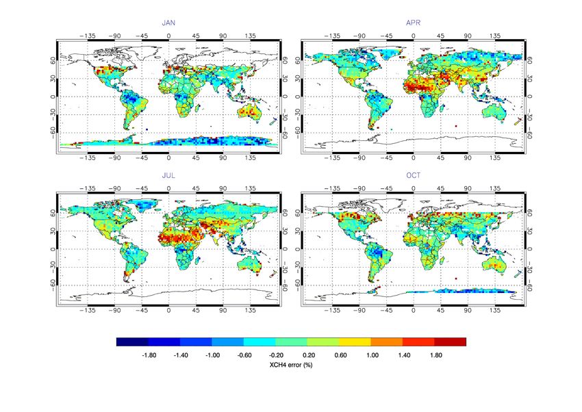
16 Relative precision of X CH4 due to the instrument noise for the a posteriori filtered dataset. 47
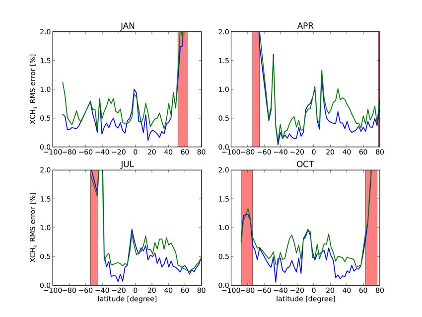
17 RMS error of X CH4 for the simulation run with ∆FWHMNIR = -1% and ∆FWHMSWIR =+1%
(green line), compared to the reference retrieval (blue line). The red areas indicate regions
with high SZA that we plan to filter out. . . . . . . . . . . . . . . . . . . . . . . . . . . . . . . . . . . . . . . . . . . . . . . . . . . . . . . . . . . 48
18 RMS error of X CH4 retrieval per latitude bin for reference retrieval (blue), offsetted by 0.1%
of the continuum but not fitted (green), and offsetted plus fitted (red). The red areas indicate
regions with high SZA that we plan to filter out. . . . . . . . . . . . . . . . . . . . . . . . . . . . . . . . . . . . . . . . . . . . . . . . . . 50
19 Same as Figure 18 but for an offset of 0.5%.. . . . . . . . . . . . . . . . . . . . . . . . . . . . . . . . . . . . . . . . . . . . . . . . . . . . 51
20 RMS of relative precision of X CH4 retrievals per latitude bin for reference retrieval (blue),
offsetted (by 0.1% of the continuum) but not fitted (green), and offsetted plus fitted (red). The
red areas indicate regions with high SZA that we plan to filter out. . . . . . . . . . . . . . . . . . . . . . . . . . . . . 52
21 RMS error of X CH4 when all instrument errors considered here are applied to the synthetic
spectra (green line), compared to reference retrieval (blue line). The retrieval settings are the
same for both simulation runs. The red areas indicate regions with high SZA that we plan to
filter out. . . . . . . . . . . . . . . . . . . . . . . . . . . . . . . . . . . . . . . . . . . . . . . . . . . . . . . . . . . . . . . . . . . . . . . . . . . . . . . . . . . . . . . . . . . . 53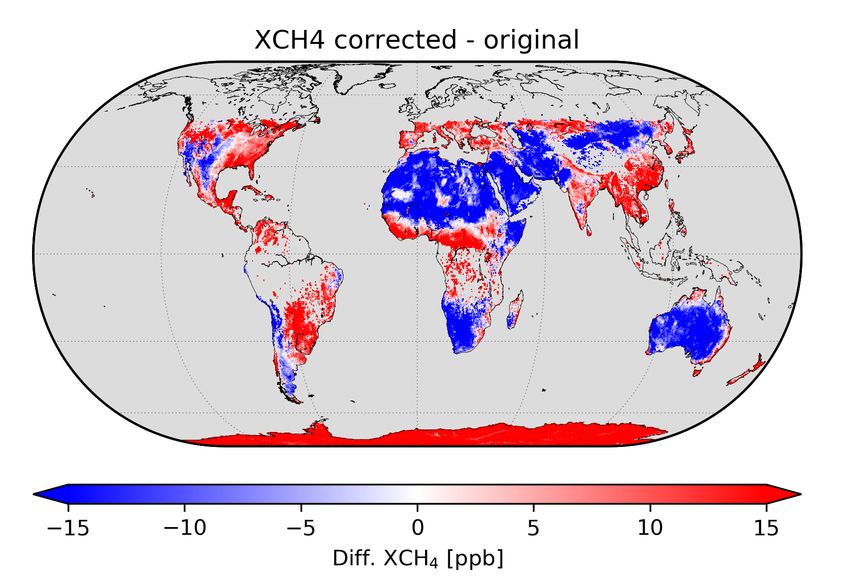
S5P ATBD draft SRON-S5P-LEV2-RP-001
issue 1.10, 2019-02-01 – released Page 8 of 67
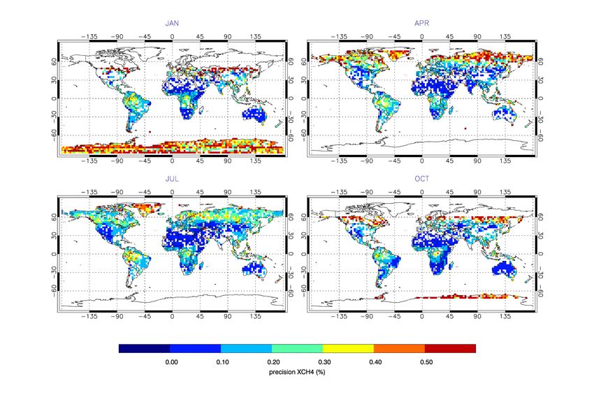
22 Forward model error of X CH4 after applying the a posteriori filters and the a priori cloud filter
based on non scattering H2 O and CH4 retrievals. . . . . . . . . . . . . . . . . . . . . . . . . . . . . . . . . . . . . . . . . . . . . . 54
23 Cumulative probability distribution of the absolute X CH4 retrieval error for the reference
retrieval that includes scattering of aerosols and cirrus for the baseline filter, baseline and
an additional filter based on non scattering CH4 retrievals, baseline and an additional filter
based on non-scattering H2 O retrievals, and the baseline and both CH4 and H2 O filters. . 55
24 Difference in retrieved columns between weak and strong absorption bands for non-scattering
atmosphere for CH4 (solid) and H2 O (dotted). For the creation of synthetic measurements a
cloud with optical thickness 5 was used with cloud top height = 2 km and cloud geometrical
thickness =1 km.. . . . . . . . . . . . . . . . . . . . . . . . . . . . . . . . . . . . . . . . . . . . . . . . . . . . . . . . . . . . . . . . . . . . . . . . . . . . . . . . . . . 55
25 Aerosol filter f value versus cloud fraction. Cases with f>110 will be filtered out, which roughly
corresponds to a cloud fraction of 0.08. . . . . . . . . . . . . . . . . . . . . . . . . . . . . . . . . . . . . . . . . . . . . . . . . . . . . . . . . . 56
26 RMS X CH4 error as a function of fluorescence emission for retrievals with and without
fluorescence included in the fit. . . . . . . . . . . . . . . . . . . . . . . . . . . . . . . . . . . . . . . . . . . . . . . . . . . . . . . . . . . . . . . . . . . 56
27 Range of the central 80% of the land albedo values in an area of about 500 × 500 km2 around
each TCCON station, except Ascension Island, for which no land data is available. A dot
indicates the median value. Sea values are excluded, but they may contaminate coastal land. 60
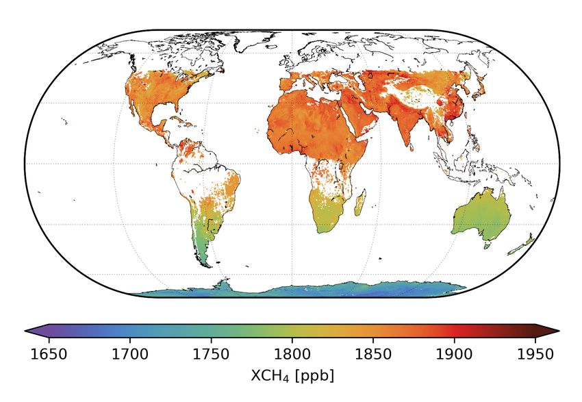
28 CH4 total column mixing ratio bias corrected of TROPOMI averaged from November 28th
2018 to January 16th 2019 . . . . . . . . . . . . . . . . . . . . . . . . . . . . . . . . . . . . . . . . . . . . . . . . . . . . . . . . . . . . . . . . . . . . . . . 61
29 Time series of daily mean X CH4 measured by TROPOMI (red dots) and by TCCON stations
(red dots) in (a) Orleans, France (left) and (b) Pasadena, U.S. (right). . . . . . . . . . . . . . . . . . . . . . . . . 62
30 (a) Station mean bias (TROPOMI-TCCON) between co-located daily mean bias-corrected
X CH4 from TROPOMI and TCCON with a global bias of -4.3 ppb and a stattion-to-station
bias variation of 7.4 ppb , (b) the station standard deviation of the bias with a station-to-station
variation of 10.2 ppb and (c) the number of coincident daily mean pairs. Data used for this
comparison ranges from May to September 2018. . . . . . . . . . . . . . . . . . . . . . . . . . . . . . . . . . . . . . . . . . . . . . 62
31 Global distribution of Aerosol Optical Thickness (AOT) adopted for the synthetic ensemble.
January (top left), April (top right), July (bottom left), and October (bottom right). . . . . . . . . . . . . 66
32 Global distribution of Cirrus Optical Thickness (COT) as used in the ensemble calculations. 66
33 Surface albedo maps in the SWIR range for the synthetic ensemble. . . . . . . . . . . . . . . . . . . . . . . . . . 67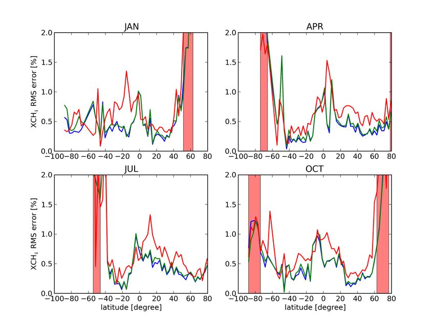
S5P ATBD draft                                                                          SRON-S5P-LEV2-RP-001
issue 1.10, 2019-02-01 – released                                                                 Page 9 of 67

1     Introduction
1.1   Identification
This document describes the algorithm for the retrieval of the column average dry air mixing ratio of methane,
X CH4 , from Sentinel-5 (S5) measurements in the Near Infra Red (NIR) and Short Wave Infra Red (SWIR)
spectral range. The algorithm name is RemoTeC-S5 and it is one of the deliverables of the ESA project
’Sentinel-5 P level 2 processor development’ [AD1].

1.2   Purpose and objectives
The purpose of the document is to describe the theoretical baseline of the algorithm that will be used to
for the operational processing to retrieve the column average dry air mixing ratio of methane X CH4 , from
Sentinel-5 Precursor (S5-P) measurements, the input and ancillary data that is needed, and the output that
will be generated. In addition, information about expected calculation times and the expected accuracy are
provided.

1.3   Document overview
Chapter 4 describes the main characteristics of the TROPOMI instrument, which was launched in October
2017. Chapter 4 gives a brief introduction to satellite X CH4 retrieval. Chapter 5 provides the description of the
baseline retrieval algorithm. In Chapter 6 the feasibility is discussed including the efficiency of the calculations.
Chapter 7 gives a detailed error analysis, Chapter 8 discusses the validation possibilities and needs, and
Chapter 9 gives some examples of TROPOMI X CH4 data. Finally, Chapter 10 concludes the document.
S5P ATBD draft                                                                     SRON-S5P-LEV2-RP-001
issue 1.10, 2019-02-01 – released                                                           Page 10 of 67

2     Applicable and reference documents
2.1   Applicable documents
[AD1] Sentinel-5P Level 2 Processor Development – Statement of Work.
      source: ESA; ref: S5P-SWESA-GS-053; date: 2012.

[AD2] GMES Sentinels 4 and 5 mission requirements document.
      source: ESA; ref: EOP-SMA/1507/JL-dr; date: 2011.

2.2   Standard documents
[SD1] Space Engineering – Software.
      source: ESA; ref: ECSS-Q-ST-80C; date: 2009.

[SD2] Space Product Assurance – Software Product Assurance.
      source: ESA; ref: ECSS-E-ST-40C; date: 2009.

[SD3] TROPOMI Instrument and Performance Overview.
      source: KNMI; ref: S5P-KNMI-L2-0010-RP; issue: 0.10.0; date: 2014.

[SD4] Requirements for the Geophysical Validation of Sentinel-5 Precursor Products, draft version.
      source: ESA; ref: S5P-RS-ESA-SY-164; date: 2014.

2.3   Reference documents
 [RD1] Terms, definitions and abbreviations for TROPOMI L01b data processor.
       source: KNMI; ref: S5P-KNMI-L01B-0004-LI; date: 2011.

 [RD2] Terms and symbols in the TROPOMI algorithm team.
       source: KNMI; ref: SN-TROPOMI-KNMI-049; date: 2012.

 [RD3] S. Solomon, D. Qin, M. Manning et al. (editors) IPCC, Climate Change 2007: The Physical Science
       Basis. Contribution of Working Group I to the Fourth Assessment Report of the Intergovernmental
       Panel on Climate Change (Cambridge University Press, Cambridge, United Kingdom and New York,
       NY, USA, 2007).

 [RD4] H. Bovensmann, J. P. Burrows, M. Buchwitz et al.; SCIAMACHY: Mission Objectives and Measurement
       Modes. Journal of Atmospheric Sciences; 56 (1999), 127.

 [RD5] T. Yokota, H. Oguma, I. Morino et al.; Test measurements by a BBM of the nadir-looking SWIR FTS
       aboard GOSAT to monitor CO2 column density from space. In Passive Optical Remote Sensing of
       the Atmosphere and Clouds IV (edited by S. C. Tsay, T. Yokota and M.-H. Ahn); volume 5652 of
       Proceedings of the SPIE; (pp. 182–188) (2004); doi:10.1117/12.578497.

 [RD6] A. Kuze, H. Suto, M. Nakajima et al.; Thermal and near infrared sensor for carbon observation
       Fourier-transform spectrometer on the Greenhouse Gases Observing Satellite for greenhouse gases
       monitoring. Appl. Opt.; 48 (2009), 6716; doi:10.1364/AO.48.006716.

 [RD7] J. F. Meirink, H. J. Eskes and A. P. H. Goede; Sensitivity analysis of methane emissions derived from
       SCIAMACHY observations through inverse modelling. Atmos. Chem. Phys.; 6 (2006), 1275.

 [RD8] P. Bergamaschi, C. Frankenberg, J. F. Meirink et al.; Satellite chartography of atmospheric methane
       from SCIAMACHY on board ENVISAT: 2. Evaluation based on inverse model simulations. J. Geophys.
       Res.; 112 (2007), D02304; doi:10.1029/2006JD007268.

 [RD9] A. Butz, O. P. Hasekamp, C. Frankenberg et al.; CH4 retrievals from space-based solar backscatter
       measurements: Performance evaluation against simulated aerosol and cirrus loaded scenes. J.
       Geophys. Res.; 115 (2010), D24302; doi:10.1029/2010JD014514.

[RD10] I. Aben, O. Hasekamp and W. Hartmann; Uncertainties in the space-based measurements of CO2
       columns due to scattering in the Earth’s atmosphere. J. Quant. Spectrosc. Radiat. Transfer; 104 (2007),
       450; doi:10.1016/j.jqsrt.2006.09.013.
S5P ATBD draft SRON-S5P-LEV2-RP-001
issue 1.10, 2019-02-01 – released Page 11 of 67
[RD11] A.M.S. Gloudemans, H. Schrijver, O.P. Hasekamp et al.; Error analysis for CO and CH4 total column
retrieval from SCIAMACHY 2.3µm spectra. Atmos. Chem. Phys.; 8 (2008), 3999.
[RD12] C Frankenberg, U. Platt and T. Wagner; Retrieval of CO from SCIAMACHY onboard ENVISAT:
detection of strongly polluted areas and seasonal patterns in global CO abundances. Atmos. Chem.
Phys.; 4 (2005), 8425.
[RD13] C. Frankenberg, P. Bergamaschi, A. Butz et al.; Tropical methane emissions: A revised view from
SCIAMACHY onboard ENVISAT. Geophys. Res. Lett.; 35 (2008), 15811; doi:10.1029/2008GL034300.
[RD14] O. Schneising, M. Buchwitz, M. Reuter et al.; Long-term analysis of carbon dioxide and methane
column-averaged mole fractions retrieved from SCIAMACHY. Atmos. Chem. Phys.; 11 (2011), 2863;
doi:10.5194/acp-11-2863-2011.
[RD15] R. Parker, H. Boesch, A. Cogan et al.; Methane observations from the Greenhouse Gases Observing
SATellite: Comparison to ground-based TCCON data and model calculations. Geophys. Res. Lett.; 38
(2011), L15807; doi:10.1029/2011GL047871.
[RD16] D. Schepers, S. Guerlet, A. Butz et al.; Methane retrievals from Greenhouse Gases Observing Satellite
(GOSAT) shortwave infrared measurements: Performance comparison of proxy and physics retrieval
algorithms. J. Geophys. Res.; 117 (2012), D10307; doi:10.1029/2012JD017549.
[RD17] H. BöSch, G. C. Toon, B. Sen et al.; Space-based near-infrared CO2 measurements: Testing the Orbit-
ing Carbon Observatory retrieval algorithm and validation concept using SCIAMACHY observations
over Park Falls, Wisconsin. J. Geophys. Res.; 111 (2006), D23302; doi:10.1029/2006JD007080.
[RD18] B. J. Connor, H. Boesch, G. Toon et al.; Orbiting Carbon Observatory: Inverse method and prospective
error analysis. J. Geophys. Res.; 113 (2008), D05305; doi:10.1029/2006JD008336.
[RD19] S. Oshchepkov, A. Bril and T. Yokota; PPDF-based method to account for atmospheric light scat-
tering in observations of carbon dioxide from space. J. Geophys. Res.; 113 (2008), D23210;
doi:10.1029/2008JD010061.
[RD20] A. Butz, O. P. Hasekamp, C. Frankenberg et al.; Retrievals of atmospheric CO_2 from simulated
space-borne measurements of backscattered near-infrared sunlight: accounting for aerosol effects.
Appl. Opt.; 48 (2009), 3322; doi:10.1364/AO.48.003322.
[RD21] A. Bril, S. Oshchepkov and T. Yokota; Retrieval of atmospheric methane from high spectral res-
olution satellite measurements: a correction for cirrus cloud effects. Appl. Opt.; 48 (2009), 2139;
doi:10.1364/AO.48.002139.
[RD22] M. Reuter, M. Buchwitz, O. Schneising et al.; A method for improved SCIAMACHY CO2 retrieval in the
presence of optically thin clouds. Atmos. Meas. Tech.; 3 (2010), 209.
[RD23] A. Butz, S. Guerlet, O. Hasekamp et al.; Toward accurate CO2 and CH4 observations from GOSAT.
Geophys. Res. Lett.; 38 (2011), doi:10.1029/2011GL047888.
[RD24] H. Boesch, D. Baker, B. Connor et al.; Global Characterization of CO2 Column Retrievals from
Shortwave-Infrared Satellite Observations of the Orbiting Carbon Observatory-2 Mission. Remote
Sens. Envirom.; 3 (2011), 270; doi:10.3390/rs3020270.
[RD25] Y. Yoshida, Y. Ota, N. Eguchi et al.; Retrieval algorithm for CO2 and CH4 column abundances from
short-wavelength infrared spectral observations by the Greenhouse gases observing satellite. Atmos.
Meas. Tech.; 4 (2011), 717; doi:10.5194/amt-4-717-2011.
[RD26] C. W. O’Dell, B. Connor, H. Bösch et al.; The ACOS CO2 retrieval algorithm - Part 1: Description and
validation against synthetic observations. Atmos. Meas. Tech.; 5 (2012), 99; doi:10.5194/amt-5-99-
2012.
[RD27] O. P. Hasekamp and A. Butz; Efficient calculation of intensity and polarization spectra in vertically
inhomogeneous scattering and absorbing atmospheres. J. Geophys. Res.; 113 (2008), D20309;
doi:10.1029/2008JD010379.S5P ATBD draft SRON-S5P-LEV2-RP-001
issue 1.10, 2019-02-01 – released Page 12 of 67
[RD28] S. Guerlet, A. Butz, D. Schepers et al.; Impact of aerosol and thin cirrus on retrieving and valid-
ating XCO2 from GOSAT shortwave infrared measurements. J. Geophys. Res.; 118 (2013), 4887;
doi:10.1002/jgrd.50332.
[RD29] S. Guerlet, S. Basu, A. Butz et al.; Reduced carbon uptake during the 2010 Northern Hemisphere
summer from GOSAT. Geophys. Res. Lett.; 40 (2013), 2378; doi:10.1002/grl.50402.
[RD30] J.P. Veefkind, I. Aben, K. McMullan et al.; TROPOMI on the ESA Sentinel-5 Precursor: A GMES
mission for global observations of the atmospheric composition for climate, air quality and ozone layer
applications. Remote Sens. Envirom.; 120 (2012), 70; doi:doi:10.1016/j.rse.2011.09.027.
[RD31] R. van Deelen, O. P. Hasekamp and J. Landgraf; Accurate modeling of spectral fine-structure in Earth
radiance spectra measured with the Global Ozone Monitoring Experiment. Appl. Opt.; 46 (2007), 243;
doi:10.1364/AO.46.000243.
[RD32] D. Wunch, G. C. Toon, P. O. Wennberg et al.; Calibration of the Total Carbon Column Observing Network
using aircraft profile data. Atmospheric Measurement Techniques; (2010), 1351; doi:10.5194/amt-3-
1351-2010.
[RD33] A. Jenouvrier, L. Daumont, L. Régalia-Jarlot et al.; Fourier transform measurements of water vapor
line parameters in the 4200 6600 cm−1 region. J. Quant. Spectrosc. Radiat. Transfer; 105 (2007), 326;
doi:10.1016/j.jqsrt.2006.11.007.
[RD34] L.S. Rothman, I.E. Gordon, A. Barbe et al.; The HITRAN 2008 molecular spectroscopic database. J.
Quant. Spectrosc. Radiat. Transfer; 110 (2009), 533.
[RD35] R. A. Scheepmaker, C. Frankenberg, A. Galli et al.; Improved water vapour spectroscopy in the
4174–4300 cm−1 region and its impact on SCIAMACHY HDO/H2 O measurements. Atmos. Meas.
Tech.; 6 (2013) (4), 879; doi:10.5194/amt-6-879-2013. URL http://www.atmos-meas-tech.net/6/
879/2013/.
[RD36] H. Tran, C. Boulet and J.-M. Hartmann; Line mixing and collision-induced absorption by oxygen in
the A band: Laboratory measurements, model, and tools for atmospheric spectra computations. J.
Geophys. Res.; 111 (2006), D15210; doi:10.1029/2005JD006869.
[RD37] A. Bucholtz; Rayleigh-Scattering calculations for the terrestrial atmosphere. Appl. Opt.; 35 (1995),
2765.
[RD38] J. E. Hansen and L. D. Travis; Light scattering in planetary atmospheres. Space Science Reviews; 16
(1974), 527; doi:10.1007/BF00168069.
[RD39] M. I. Mishchenko, I. V. Geogdzhayev, B. Cairns et al.; Aerosol retrievals over the ocean by use of
channels 1 and 2 AVHRR data: sensitivity analysis and preliminary results. Appl. Opt.; 38 (1999),
7325; doi:10.1364/AO.38.007325.
[RD40] P. Stier, J. Feichter, S. Kinne et al.; The aerosol-climate model ECHAM5-HAM. Atmos. Chem. Phys.; 5
(2005), 1125.
[RD41] O. Dubovik, A. Sinyuk, T. Lapyonok et al.; Application of spheroid models to account for aerosol
particle nonsphericity in remote sensing of desert dust. J. Geophys. Res.; 111 (2006), D11208;
doi:10.1029/2005JD006619.
[RD42] J. F. de Haan, P. B. Bosma and J. W. Hovenier; The adding method for multiple scattering calculations
of polarized light. Astron. and Astrophys.; 183 (1987), 371.
[RD43] J. Landgraf, O.P. Hasekamp, M. Box et al.; A Linearized Radiative Transfer Model Using the Analytical
Perturbation Approach. J. Geophys. Res.; 106 (2001), 27291.
[RD44] O. P. Hasekamp and J. Landgraf; Linearization of vector radiative transfer with respect to aer-
osol properties and its use in satellite remote sensing. J. Geophys. Res.; 110 (2005), D04203;
doi:10.1029/2004JD005260.
[RD45] B. van Diedenhoven, O. P. Hasekamp and J. Landgraf; Efficient vector radiative transfer
calculations in vertically inhomogeneous cloudy atmospheres. Appl. Opt.; 45 (2006), 5993;
doi:10.1364/AO.45.005993.S5P ATBD draft SRON-S5P-LEV2-RP-001
issue 1.10, 2019-02-01 – released Page 13 of 67
[RD46] M. Duan, Q. Min and J. Li; A fast radiative transfer model for simulating high-resolution absorption
bands. J. Geophys. Res.; 110 (2005) (D15); doi:10.1029/2004JD005590. D15201; URL http://dx.
doi.org/10.1029/2004JD005590.
[RD47] C. Frankenberg, C. O’Dell, L. Guanter et al.; Remote sensing of near-infrared chlorophyll fluorescence
from space in scattering atmospheres: implications for its retrieval and interferences with atmospheric
CO2 retrievals. Atmos. Meas. Tech.; 5 (2012), 2081; doi:10.5194/amt-5-2081-2012.
[RD48] P.L. Phillips; A technique for the numerical solution of certain integral equations of the first kind. J. Ass.
Comput. Mat.; 9 (1962), 84.
[RD49] A.N. Tikhonov; On the solution of incorrectly stated problems and a method of regularization. Dokl.
Acad. Nauk SSSR; 151 (1963), 501.
[RD50] P. C. Hansen; Rank-deficient and discrete ill-posed problems (SIAM, Philadephia, 1998).
[RD51] C. D. Rodgers and B. J. Connor; Intercomparison of remote sounding instruments. Journal of Geo-
physical Research (Atmospheres); 108 (2003), 4116; doi:10.1029/2002JD002299.
[RD52] C.D. Rodgers; Inverse Methods for Atmospheres: Theory and Practice; volume 2 (World Scientific,
2000).
[RD53] S5P-NPP Cloud Processor ATBD, issue 0.13.0.
source: RAL; ref: S5P-NPPC-RAL-ATBD-0001; date: 2015.
[RD54] Algorithm Theoretical Baseline Document for Sentinel-5 Precursor: Carbon Monoxide Total Column
Retrieval.
source: SRON; ref: SRON-S5P-LEV2-RP-002; date: 2016.
[RD55] B. van Diedenhoven, O. P. Hasekamp and I. Aben; Surface pressure retrieval from SCIAMACHY
measurements in the O2 A Band: validation of the measurements and sensitivity on aerosols. Atmos.
Chem. Phys.; 5 (2005), 2109.
[RD56] ATBD for S5P inter channel co-registration.
source: SRON; ref: SRON-S5P-LEV2-TN-018; date: 2014.
[RD57] M. Inoue, I. Morino, O. Uchino et al.; Bias corrections of GOSAT SWIR XCO2 and XCH4 with TCCON
data and their evaluation using aircraft measurement data. Atmospheric Measurement Techniques; 9
(2016), 3491; doi:10.5194/amt-9-3491-2016.
[RD58] L. Wu, O. Hasekamp, H. Hu et al.; Carbon dioxide retrieval from OCO-2 satellite observations using
the RemoTeC algorithm and validation with TCCON measurements. Atmospheric Measurement
Techniques; 11 (2018), 3111; doi:10.5194/amt-11-3111-2018.
[RD59] ESA Climate Change Initiative (CCI): Product User Guide (PUG) for the RemoTeC XCH4 PROXY
GOSAT Data Product v2.3.8 for the Essential Climate Variable (ECV) Greenhouse Gases (GHG).
source: SRON Netherlands Insitute for Space Research; ref: Version 4.1; date: 2016.
[RD60] M. Hess, R. B. A. Koelemeijer and P. Stammes; Scattering matrices of imperfect hexagonal ice
crystals. Journal of Quantitative Spectroscopy and Radiative Transfer; 60 (1998), 301 ; doi:DOI:
10.1016/S0022-4073(98)00007-7.
[RD61] A. Galli, A. Butz, R. A. Scheepmaker et al.; CH4 , CO, and H2 O spectroscopy for the Sentinel-5
Precursor mission: an assessment with the Total Carbon Column Observing Network measurements.
Atmos. Meas. Tech.; 5 (2012), 1387; doi:10.5194/amt-5-1387-2012.
[RD62] A. Butz, A Galli, O.P. Hasekamp et al.; ROPOMI aboard Sentinel-5 Precursor: Prospective performance
of CH4 retrievals for aerosol and cirrus loaded atmospheres. Remote Sens. Envirom.; 120 (2012), 267.
[RD63] GMES Sentinel-5 Precursor – S5p System Requirement Document.
source: ESA; ref: S5p-RS-ESA-SY-0002; date: 2011.
[RD64] D Wunch, G. C Toon, J.-F. L Blavier et al.; The Total Carbon Column Observing Network. Philos. T. R.
Soc. A.; 369 (2011) (1943), 2087; doi:10.1098/rsta.2010.0240.S5P ATBD draft SRON-S5P-LEV2-RP-001
issue 1.10, 2019-02-01 – released Page 14 of 67
[RD65] M. Reuter, H. Bösch, H. Bovensmann et al.; A joint effort to deliver satellite retrieved atmospheric
CO2 concentrations for surface flux inversions: the ensemble median algorithm EMMA. Atmos. Chem.
Phys.; 13 (2013), 1771; doi:10.5194/acp-13-1771-2013.
[RD66] C. Petri, T. Warneke, N. Jones et al.; Remote sensing of CO2 and CH4 using solar absorption
spectrometry with a low resolution spectrometer. Atmos. Meas. Tech.; 5 (2012), 1627; doi:10.5194/amt-
5-1627-2012.
[RD67] M. Gisi, F. Hase, S. Dohe et al.; XCO2 -measurements with a tabletop FTS using solar absorption
spectroscopy. Atmos. Meas. Tech.; 5 (2012), 2969; doi:10.5194/amt-5-2969-2012.
[RD68] A. Karion, C. Sweenney, P. Tans et al.; AirCore: An Innovative Atmospheric Sampling System. J. Atm.
Ocean Tech.; 27 (2010), 1839; doi:doi:10.1175/2010JTECHA1448.1.
[RD69] H. Hu, J. Landgraf, R. Demeters et al.; Toward Global Mapping of Methane With TROPOMI:
First Results and Intersatellite Comparison to GOSAT. Geophys. Res. Lett.; 45 (2018), 3682;
doi:10.1002/2018GL077259.
[RD70] S5P Mission Performance Centre Methane [L2__CH4___] Readme.
source: ; ref: Version 1.02.02, S5P-MPC-SRON-PRF-CH4; date: 2019.
[RD71] O.P. Hasekamp and J. Landgraf; A linearized vector radiative transfer model for atmospheric trace gas
retrieval. J. Quant. Spectrosc. Radiat. Transfer; 75 (2002).
[RD72] M. Hess and M. Wiegner; COP: a data library of optical properties of hexagonal ice crystals. Appl.
Opt.; 33 (1994) (33), 7740; doi:10.1364/AO.33.007740.
[RD73] A. J. Heymsfield and C. M. R. Platt; A Parameterization of the Particle Size Spectrum of Ice Clouds
in Terms of the Ambient Temperature and the Ice Water Content. J. Atmos. Sci.; 41 (1984), 846;
doi:10.1175/1520-0469(1984)0412.0.CO;2.
[RD74] D. M. Winker, W. H. Hunt and M. J. McGill; Initial performance assessment of CALIOP. Geophys. Res.
Lett.; 34 (2007), L19803; doi:10.1029/2007GL030135.
[RD75] H. Schrijver, A. M. S. Gloudemans, C. Frankenberg et al.; Water vapour total columns from SCIA-
MACHY spectra in the 2.36 µm window. Atmos. Meas. Tech.; 2 (2009), 561.
[RD76] C. Popp, P. Wang, D. Brunner et al.; MERIS albedo climatology for FRESCO+ O2 A-band cloud
retrieval. Atmospheric Measurement Techniques; 4 (2011), 463; doi:10.5194/amt-4-463-2011.
2.4 Electronic references
There are no electronic referencesS5P ATBD draft SRON-S5P-LEV2-RP-001 issue 1.10, 2019-02-01 – released Page 15 of 67 3 Terms, definitions and abbreviated terms Terms, definitions and abbreviated terms that are used in the development program for the TROPOMI L0 1b data processor are described in [RD1]. Terms, definitions and abbreviated terms that are used in development program for the TROPOMI L2 data processors are described in [RD2]. Terms, definitions and abbreviated terms that are specific for this document can be found below. 3.1 Acronyms and abbreviations ECMWF European Centre for Medium-Range Weather Forecasts ENVISAT Environmental Monitoring Satellite GOSAT Greenhouse gas Observing SATtellite NASA National Aeronautics and Space Administration NOAA National Oceanic and Atmospheric Administration NPP NPOESS Prepatory Project NIR Near Infra Red OCO Orbiting Carbon Observatory SCIAMACHY SCanning Imaging Absorption SpectroMeter for Atmospheric CHartographY SWIR Short Wave Infra Red S5P Sentinel-5 Precursor TCCON Total Carbon Column Observing Network TROPOMI Tropospheric Monitoring Instrument UVN Ultraviolet, Visible, Near-Infrared VIIRS Visible Infrared Imaging Radiometer Suite XCH4 Column averaged dry air mixing ratio of methane
S5P ATBD draft                                                                         SRON-S5P-LEV2-RP-001
issue 1.10, 2019-02-01 – released                                                               Page 16 of 67

4     Introduction to methane retrieval algorithm
4.1   Background
Methane (CH4 ) is, after carbon dioxide (CO2 ), the most important contributor to the anthropogenically enhanced
greenhouse effect [RD3]. Monitoring CH4 abundances in the Earth’s atmosphere is the dedicated goal of
several current and future satellite missions. Such space borne observations aim at providing CH4 column
concentrations with high sensitivity at the Earth’s surface, with good spatiotemporal coverage, and with sufficient
accuracy to facilitate inverse modeling of sources and sinks. The Scanning Imaging Absorption Spectrometer
for Atmospheric Chartography (SCIAMACHY) on board ENVISAT [RD4], that was operational 2002-2012, and
the Greenhouse Gases Observing Satellite (GOSAT) [RD5], [RD6], launched 2009, have the capability to
achieve these goals. Their observation strategy relies on measuring spectra of sunlight backscattered by the
Earth’s surface and atmosphere in the shortwave infrared (SWIR) spectral range. Absorption features of CH4
allow for retrieval of its atmospheric concentration with high sensitivity to the ground and the lower atmosphere
where the major CH4 sources are located. The benefit of such measurements for estimating source/sink
strengths, however, strongly depends on the precision and accuracy achieved. When correlated on the regional
or seasonal scale, systematic biases of a few tenths of a percent can jeopardize the usefulness of satellite-
measured CH4 concentrations for source/sink estimates [RD7, RD8, RD9]. Scattering by aerosols and cirrus
clouds is the major challenge for retrievals of methane from space-borne observations of backscattered sunlight
in the SWIR spectral range. While contamination by optically thick clouds can be filtered out reliably, optically
thin scatterers are much harder to detect yet still modify the light path of the observed backscattered sunlight and
thus, can lead to underestimation or overestimation of the true methane column if not appropriately accounted
for. The net light path effect strongly depends on the amount, the microphysical properties, and the height
distribution of the scatterers as well as on the reflectance of the underlying ground surface [RD10, RD11].
Therefore, retrieval strategies rely on inferring the targeted gas concentration either simultaneously with
scattering properties of the atmosphere or with a light path proxy. The latter ‘proxy’ approach has been
successfully implemented for methane retrieval from SCIAMACHY measurements around 1600 nm, by using
the CO2 column, also retrieved from SCIAMACHY in the same spectral range, as a lightpath proxy [RD12].
The ‘proxy’ approach relies on the assumptions that scattering effects cancel in the ratio of the methane column
and the CO2 column and that a prior estimate of the CO2 column is sufficiently accurate to reliably re-calculate
the methane column from the ratio. By definition, the accuracy of the ‘proxy’ approach is contingent on the
uncertainty of CO2 column used for rescaling and on the cancellation of errors in the CH4 /CO2 ratio. Further
applications of the proxy approach for methane retrieval from SCIAMACHY are described by Frankenberg et
al., 2018 [RD13] and Schneising et al., 2011 [RD14]. For GOSAT, the proxy approach has been successfully
applied by Parker et al., 2011 [RD15] and Schepers et al., 2012 [RD16].
     Alternatively, scattering induced lightpath modification can be taken into account by simultaneously inferring
the atmospheric CH4 concentration and physical scattering properties of the atmosphere. Such ‘physics-based’
methods have been developed for space-based CO2 and/or CH4 measurements from SCIAMACHY, GOSAT,
and the Orbiting Carbon Observatory (OCO) (e.g. [RD17, RD18, RD19, RD20, RD21, RD22, RD23, RD24,
RD25, RD26]). The physics based methods make use of the Oxygen A-band around 760 nm and absorption
bands of the target absorber (CH4 and/or CO2 ) in the SWIR spectral range. The advantage of physics based
methods for methane retrieval compared to a proxy method is that they do not depend on accurate prior
information on the CO2 column. On the other hand, the physics based algorithms are more complex and may
be limited by the information content of the measurement with respect to aerosol properties and/or forward
model errors in the description of aerosols. A detailed comparison between the two methods for GOSAT is
provided by Schepers et al., 2012 [RD16].

4.2   The S5P spectral range
The spectral range measured by the S5P instrument [SD3] does not allow for a light-path-proxy approach, and
thus the effect of aerosols and cirrus should be accounted for using a physics based method as mentioned
above. The spectral ranges to be used are shown in Figure 1. The algorithm retrieves 3 aerosol parameters
(amount, size, height) simultaneously with the methane column (and other parameters such as surface albedo)
in order to account for light path modification by aerosols. The information on aerosol parameters comes
from the parts of the spectrum with strong absorption lines (O2 in the NIR band, CH4 and H2 O in the SWIR
band) of which the depth and shape is modified by aerosol scattering. The basis of the algorithm is to fit a
forward model capable of handling (multiple) scattering by molecules and particles in the atmosphere, with the
approximate parameterization of atmospheric scattering properties described above to the S5P NIR and SWIR
S5P ATBD draft SRON-S5P-LEV2-RP-001
issue 1.10, 2019-02-01 – released Page 17 of 67
measurements. An important aspect of the algorithm is computational speed, since the S5P instrument will
provide significantly more measurements than earlier instruments. For this purpose we developed a highly
efficient radiative transfer model that avoids time consuming line-by-line calculations using a k-binning approach
[RD27].
Figure 1: Simulated spectrum at S5P spectral resolution for the O2 A band (left panel) and the SWIR band
(right panel).
4.3 Heritage
The algorithm for retrieval of methane columns from the S5P instrument is based on earlier developments
of a CO2 and CH4 retrieval algorithm from GOSAT, called RemoTeC [RD20, RD9, RD23, RD16, RD28],
making use of measurements at the O2 A band, and the 1600 nm and 2000 nm CO2 absorption bands. For
CO2 and CH4 retrieval from GOSAT the algorithm has been thoroughly tested for simulations where the
actual scattering properties are unknown [RD20, RD9], and has been successfully applied to real GOSAT
measurements [RD23, RD16, RD28, RD29]. For the operational S5P methane column retrieval algorithm we
build further on the RemoTeC algorithm for GOSAT. Here, the algorithm has to be adjusted to the spectral
range and spectral resolution of the S5P instrument. We cannot test the algorithm on real measurements
for the S5P spectral range (SCIAMACHY measurements do not have sufficient quality in the 2.3 µm range)
and therefore we test the S5P algorithm for an ensemble of scenarios with realistic combinations of aerosol
properties, cirrus properties, surface albedo, and solar zenith angle, similarly to what was done for GOSAT
prior to the GOSAT launch [RD9]. Since the S5P spectral range has no heritage for CH4 retrieval, it is also
important to investigate the quality of the relevant spectroscopic data in this spectral range, which is done
using ground based Fourier Transform spectroscopy measurements.
4.4 Requirements
The accuracy requirement for the column integrated dry air-mixing ratio of methane (X CH4 ) has originally been
formulated as 2% [AD2]. Veefkind et al., 2012 [RD30] formulate this requirement as 2% accuracy and 0.6%
precision (defined as the contribution of purely random instrument noise). More recently, the requirement has
been reformulated as 1% bias and 1% precision [SD4]. From the 1% bias 0.6% is reserved for instrument
related errors and 0.8% for forward model errors. It is also important to keep in mind the performance of the
Japanese GOSAT satellite, launched 2009, which sets the current benchmark for methane retrievals from space.
Performing GOSAT methane retrievals using the same algorithm as the S5P prototype algorithm [RD23, RD16],
for methane we achieve a precision of ∼0.8% per individual measurement and a relative accuracy (between
regions) of ∼0.25%.
Given the large number of measurement provided by the S5P instrument, the requirement on processing
speed is very demanding. Taking into account that only cloud-free measurements over land will be processed,
which is ∼3% of the total daytime data, the requirement on the processing time for a single S5P CH4 retrieval
is in the order of a few seconds assuming a reasonable amount of processing cores.S5P ATBD draft SRON-S5P-LEV2-RP-001
issue 1.10, 2019-02-01 – released Page 18 of 67
Table 1: Spectral ranges from the NIR and SWIR band included in the measurement vector
band used spectral range
NIR 757 774 nm
SWIR 2305-2385 nm
5 Algorithm description
Any retrieval algorithm aims at inferring an atmospheric state vector x from a measurement vector y. The state
vector is linked to the measurement vector through the true forward model f(x, b) that depends on the state
vector x and the vector b containing ancillary parameters that are not retrieved,
y = f(x, b) + ey (1)
where ey represents the measurement noise vector. A retrieval method approximates the true forward model f
by a retrieval forward model F, with a forward model error vector eF ,
y = F(x, b) + ey + eF . (2)
For methane retrieval from the S5P instrument the measurement vector contains the measured radiances in
the spectral ranges 757-774 nm of the Near-InfraRed (NIR) channel and 2305-2385 nm in the SWIR channel
(see Table 1).
For the retrieval procedure it is needed that the non-linear forward model is linearized so that the retrieval
problem can be solved iteratively. For iteration step n the forward model is approximated by
F(x, b) ≈ F(xn , b) + K(xn − x) , (3)
where xn is the state vector for the n-th iteration step and K is the Jacobian matrix
∂F
K= . (4)
∂x
Below, we will describe the retrieval forward model, state vector, ancillary parameter vector, and the inversion
method in more detail.
5.1 Forward model
The retrieval forward model F simulates the measurement vector y for a given model atmosphere defined by
the state vector x and the ancillary parameter vector b. The simulated radiance for a given spectral pixel i for
S5P is given by
λmax
Z
Iconv,i = I(λ) S i (λ) dλ (5)
λmin
where I(λ) is the intensity modeled by the radiative transfer code (see below), and S i (λ) is the Instrument
Spectral Response Function (ISRF) for spectral pixel i. In the NIR and SWIR channel I(λ) contains many fine
spectral structures due to molecular absorption, so it has to be calculated line-by-line at fine spectral sampling
(at least 0.1 cm−1 in the NIR band and 0.02 cm−1 in the SWIR). In discretized form we can write the convolution
with the ISRF by a matrix equation
Iconv = S Ifine (6)
where Iconv is a vector containing the intensity measurements for all spectral pixels under consideration, S is a
matrix containing the ISRF for the different spectral pixels, and Ifine is the modeled intensity spectrum at high
spectral resolution. A similar equation can be written for the convolution of the solar spectrum with the ISRF.S5P ATBD draft SRON-S5P-LEV2-RP-001
issue 1.10, 2019-02-01 – released Page 19 of 67
In order to model the intensity at high spectral resolution also a high spectral resolution solar spectrum
F0,fine is needed. We obtain F0,fine by performing a deconvolution of the measured solar spectrum F0,meas :
F0,fine = ST (SST )−1 F0,meas (7)
The advantage of using a high spectral resolution solar spectrum obtained by deconvolution of the measured
solar spectrum is that it is similarly affected by instrument features as the measured intensity spectrum. For
further details and overview of the benefits of this method see van Deelen et al., 2007 [RD31].
5.1.1 Model Atmosphere and Optical Properties
For the S5P X CH4 algorithm described here, the model atmosphere is defined for NLAY = 36 homogeneous
vertical layers that are equidistant in pressure, the largest pressure level being defined by the surface pressure.
The absorbing trace gases of interest are O2 (in the NIR band) and CH4 , H2 O, and CO in the SWIR band.
The layer sub-columns of these gases are for the first iteration step of each retrieval calculated from the input
profiles of CH4 , CO (TM5) and H2 O (ECMWF) and the temperature and pressure profiles (ECMWF). They are
obtained on the grid of the model atmosphere by linear interpolation. Here, first the surface pressure psurf is
obtained by interpolating the input pressure profile as function of height to the surface height (input) for the
corresponding ground pixel. Next the pressure values at the layer boundaries are calculated, with the pressure
pk at the lower boundary of layer k (counting from top to bottom) is given by:
plev,k = pmin + ∆p · k (8)
∆p = (psurf − pmin )/NLAY (9)
where pmin is the pressure value of the upper boundary of the input (ECMWF) atmosphere. The different
atmospheric profiles are constructed on this pressure grid. For example, the methane sub-column DV _CH4k
for the layer bounded by pressure levels plev,k−1 and plev,k is given by:
DV _CH4k = X CH4k DV _AIRk (10)
where X CH4k is the methane dry air mixing ratio linearly interpolated from the input pressure grid to the
pressure at the ‘middle’ of layer k defined by (pk + pk+1 )/2. DV _AIRk is the sub-column of air in layer k, given
by
(plev,k+1 − plev,k) R
DV _AIRk = XH O
(11)
M gk (1 + 1.60855
2 k
)
where R is Avogado’s number, M is the molecular mass of air, gk is the gravity constant in altitude layer
k, and 1.60855 is the mass of air relative to the mass of water [RD32]. The sub columns of CO and H2 O
are calculated in the same manner as for CH4 , and the O2 sub-column is obtained by multiplying the air
sub-column by the O2 mixing ratio (=0.2095).
For a radiative transfer calculation at a given wavelength the layer absorption optical thickness, scattering
optical thickness, and scattering phase function for each model layer are needed. For layer k of the model
atmosphere the CH4 absorption optical thickness at wavelength λ j is calculated by:
N
1X
τabs,CH4 (λ j ) = σ(pi , T i , λ j ) DV _CH4 (12)
N i=1
where N is the number of sub-layers in which the model atmosphere layers are divided (set at N = 2) and
σ is the absorption cross-section of CH4 at wavelength λ j , pressure pi and temperature T i at the center
of model sub-layer i. The absorption optical thickness for the other trace gases is calculated in the same
way. Pre-calculated absorption cross-sections for CH4 , CO, H2 O, and O2 are stored as lookup-table as a
function of pressure, temperature, and wavenumber. These cross-section lookup-tables are calculated from
the latest spectroscopic databases [RD33, RD34] assuming Voigt line shapes. For water vapor, an updated
spectroscopic line list has been developed by [RD35]. In the NIR spectral range the absorption cross sections
of O2 are calculated according to Tran et al., 2006 [RD36] taking into account line mixing and collision induced
absorption. The cross-section for pressure pi , temperature T i and wavelength λ j are obtained by linear
interpolation from the tabulated values. The reason that each of the NLAY layers of the model atmosphere is
further divided into N sub-layers, is to properly account for the strong dependence of temperature and pressureYou can also read