A best-practice guide to predicting plant traits from leaf-level hyperspectral data using partial least squares regression - Brookhaven National ...
←
→
Page content transcription
If your browser does not render page correctly, please read the page content below
A best-practice guide to predicting plant traits from leaf-level
hyperspectral data using partial least squares regression

Angela C Burnett, Jeremiah Anderson, Kenneth J Davidson, Kim S Ely, Julien Lamour,
Qianyu Li, Bailey D Morrison, Dedi Yang, Alistair Rogers, Shawn P Serbin

Corresponding Author
Shawn P Serbin
Email: sserbin@bnl.gov

Address for all authors
Terrestrial Ecosystem Science and Technology Group, Environmental and Climate Sciences
Department, Brookhaven National Laboratory, Upton, NY 11973, USA

ORCIDs for all authors
Angela C Burnett 0000-0002-2678-9842
Jeremiah Anderson 0000-0001-8925-5226
Kenneth J Davidson 0000-0001-5745-9689
Kim S Ely 0000-0002-3915-001X
Julien Lamour 0000-0002-4410-507X
Qianyu Li 0000-0002-0627-039X
Bailey D Morrison 0000-0001-5824-8605
Dedi Yang 0000-0003-1705-7823
Alistair Rogers 0000-0001-9262-7430
Shawn P Serbin 0000-0003-4136-8971

                                                                                         1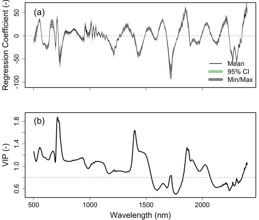
1   Highlight: We provide a step-by-step guide for combining measurements of leaf

 2   reflectance and leaf traits to build statistical models that estimate traits from reflectance,

 3   enabling rapid collection of a diverse range of leaf properties.

 4   Abstract

 5

 6   Partial least squares regression (PLSR) modelling is a statistical technique for correlating

 7   datasets, and involves the fitting of a linear regression between two matrices. One application of

 8   PLSR enables leaf traits to be estimated from hyperspectral optical reflectance data, facilitating

 9   rapid, high-throughput, non-destructive plant phenotyping. This technique is of interest and

10   importance in a wide range of contexts including crop breeding and ecosystem monitoring. The

11   lack of a consensus in the literature on how to perform PLSR means that interpreting model

12   results can be challenging, applying existing models to novel datasets can be impossible, and

13   unknown or undisclosed assumptions can lead to incorrect or spurious predictions. We address

14   this lack of consensus by proposing best practices for using PLSR to predict plant traits from

15   leaf-level hyperspectral data, including a discussion of when PLSR is applicable, and

16   recommendations for data collection. We provide a tutorial to demonstrate how to develop a

17   PLSR model, in the form of an R script accompanying this manuscript. This practical guide will

18   assist all those interpreting and using PLSR models to predict leaf traits from spectral data, and

19   advocates for a unified approach to using PLSR for predicting traits from spectra in the plant

20   sciences.

21   Keywords

22   PLSR, Spectra, Hyperspectral reflectance, Leaf traits, Plant traits, LMA, Modelling,

23   Spectroradiometer, Spectroscopy

                                                                                                          2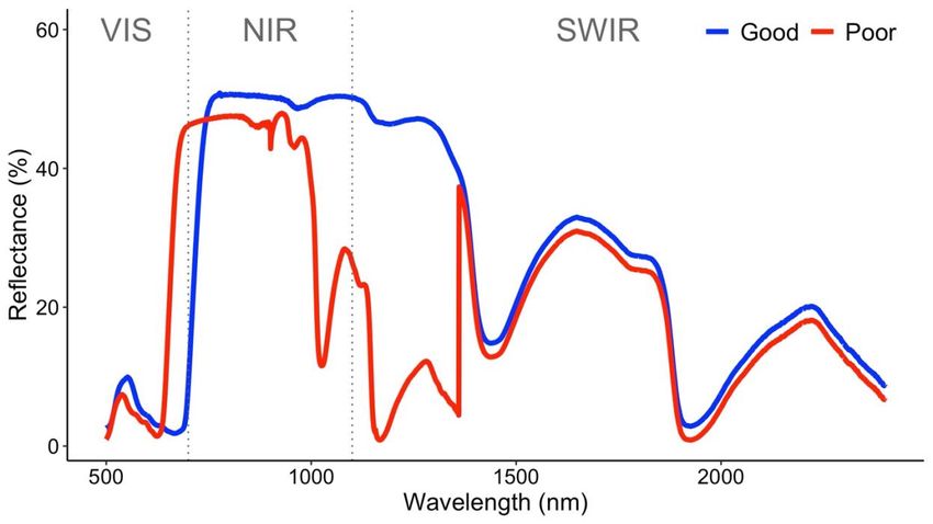
24   Introduction

25

26   Plant leaf traits are the physiological, morphological, or biochemical characteristics of plants

27   measured on individual leaves (Violle et al. 2007). Leaf traits play an important role in plant

28   resource acquisition and allocation, with broad impacts on primary production, community

29   assembly, and plant responses to climate change (Wright et al. 2004; Reich, Walters, and

30   Ellsworth 1997; Myers‐Smith, Thomas, and Bjorkman 2019; Thomas et al. 2020; Kattge et al.

31   2020). The use of leaf traits in ecological and evolutionary research has seen a dramatic

32   increase in recent years, improving our understanding of vegetation from the scale of the

33   individual plant to that of ecosystems (Woodward and Diament 1991; Violle et al. 2007;

34   Bjorkman et al. 2018). Furthermore, measuring leaf traits is a critical element of plant

35   phenotyping, including phenotyping for crop breeding and precision agriculture (Reynolds and

36   Langridge 2016). However, progress is hindered by the expensive and time-consuming

37   acquisition of traits from in-situ leaf harvesting and subsequent laboratory analysis (Cornelissen

38   et al. 2003). Laboratory processing of structural traits such as leaf mass per unit area (LMA) can

39   take days to weeks to complete, while processing leaf samples for biochemical and

40   physiological traits may take weeks to months and is also costly, requiring specialist equipment

41   and expertise. To fully extend the potential of trait-based studies, robust and non-destructive

42   methods for effectively identifying leaf traits are critically needed (Myers‐Smith, Thomas, and

43   Bjorkman 2019).

44

45   Using leaf reflectance spectra to predict leaf traits is a promising alternative to traditional

46   measurements, as reflectance can be quickly and efficiently measured using

47   spectroradiometers. A leaf reflectance spectrum results from the light absorbing and scattering

48   properties of the leaf, and is highly modified by the concentration of light absorbing compounds

                                                                                                        3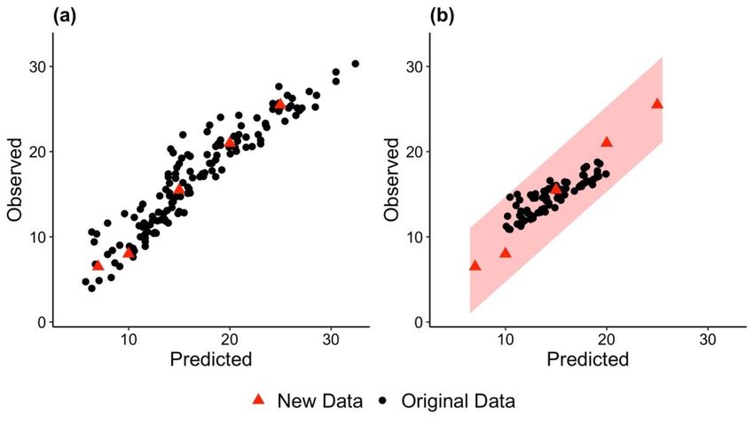
49   (photosynthetic pigments, water, cellulose, lignin, starch, protein, and macronutrients) and the

50   internal structure of leaves which determine light scattering (G. Asner 2008; Kumar et al., 2002;

51   Serbin and Townsend 2020). As leaf structure and chemical composition vary with species, age,

52   environment, and stress, these light absorbing and scattering properties change in concert (Wu

53   et al. 2017; Yang et al. 2016).

54

55   Typically, a reflectance spectrum contains a large array of variables, i.e. reflectance at different

56   spectral wavelengths, ranging from several hundred to thousands depending on the spectral

57   resolution and the range of measured wavelengths. These wavelengths typically include the

58   visible (VIS, 380–700 nm), near infrared (NIR, 700–1100 nm), and short-wave infrared (SWIR,

59   1100–2500 nm) regions, as covered by a full-range spectroradiometer. While the spectrometer

60   wavelength resolution will likely vary between detector regions, the spectral resolution is usually

61   3–5 nm in the VIS, and 6–12 in the NIR and SWIR bands, and the data is then interpolated to a

62   1 nm resolution. Given this large number of predictor variables, classic linear regression

63   modelling cannot be used due to the problems of ‘non unique solutions’ and ‘overfitting’ (Wold,

64   Sjöström, and Eriksson 2001; Geladi and Kowalski 1986). PLSR was created to handle both the

65   collinearity among predictors, in this case the different wavelengths of a reflectance spectrum,

66   and the larger number of predictor variables than trait observations. PLSR projects the highly

67   correlated predictor variables to a small number of latent variables and at the same time

68   maximizes the correlation between the response and latent variables (Wold, Sjöström, and

69   Eriksson 2001; Geladi and Kowalski 1986). This technique has been shown to be effective for

70   handling spectral data (Serbin et al. 2012, 2019; DuBois et al. 2018; Wang et al. 2020) and has

71   been successfully implemented for many types of continuous traits across a variety of growth

72   conditions, including glasshouses, farms and natural ecosystems (Meacham-Hensold et al.

73   2019; Ely et al. 2019; Wu et al. 2019). These traits include leaf structural traits, such as LMA

74   (Serbin et al. 2019); biochemical traits, such as leaf nitrogen, protein, sugars, starch and lignin

                                                                                                            4
75 (Ely et al. 2019); and physiological traits, such as the maximum carboxylation rate of Rubisco
76 (Vc,max) and maximum electron transport rate (Jmax) (Wu et al. 2019; Meacham-Hensold et al.
77 2019). These implementations of PLSR have largely improved our means for monitoring plant
78 growth and plant physiological change under environmental stress, as well as the broad trait
79 variation across vegetation types.
80
81 Previous work in the fields of chemometrics, medical sciences and sociology has provided a
82 detailed description of the mathematical aspects and advantages of PLSR over alternative
83 approaches, therefore we will not address this here (Shmueli et al. 2016; Krishnan et al. 2011;
84 Wold, Sjöström, and Eriksson 2001; Martens and Martens 2000; Sawatsky, Clyde, and Meek
85 2015). However, there is currently no clear guide on how to predict plant traits from
86 hyperspectral data, and particularly how to apply the PLSR technique (Villa et al., 2020; Polley
87 et al. 2020; Barnes et al. 2017). Whilst there are plenty of specific examples of PLSR being
88 used to predict traits from spectra, we lack a general overview of PLSR for plant ecology.
89
90 Furthermore, there are a variety of approaches available for leaf trait and hyperspectral data
91 collection, including choices of instrumentation, measurement procedures and quality control, as
92 well as different approaches for developing and validating a PLSR model, with steps including
93 sample selection, handling imbalanced data and outliers, determining the number of
94 components, and model validation. There is also a wide choice of PLSR software, such as ‘pls’
95 (R software environment), ‘plsregress’ (Matlab), ‘sklearn’ (Python), ‘PLS procedure’ in SAS,
96 Statistica, and SPSS; furthermore there are many different outputs, including figures and indices
97 of performances. Collectively, this overwhelming variety of potential pathways for analysis is
98 hindering the development of a coherent approach that can enable clear comprehension and
99 comparison of results and the sharing and application of PLSR models by the community.
100 Finally, for the researcher hoping to begin applying the PLSR technique to new questions, the
5101 absence of an established best-practice method leaves the uninitiated user unsure of how to
102 begin working with this powerful technique.
103
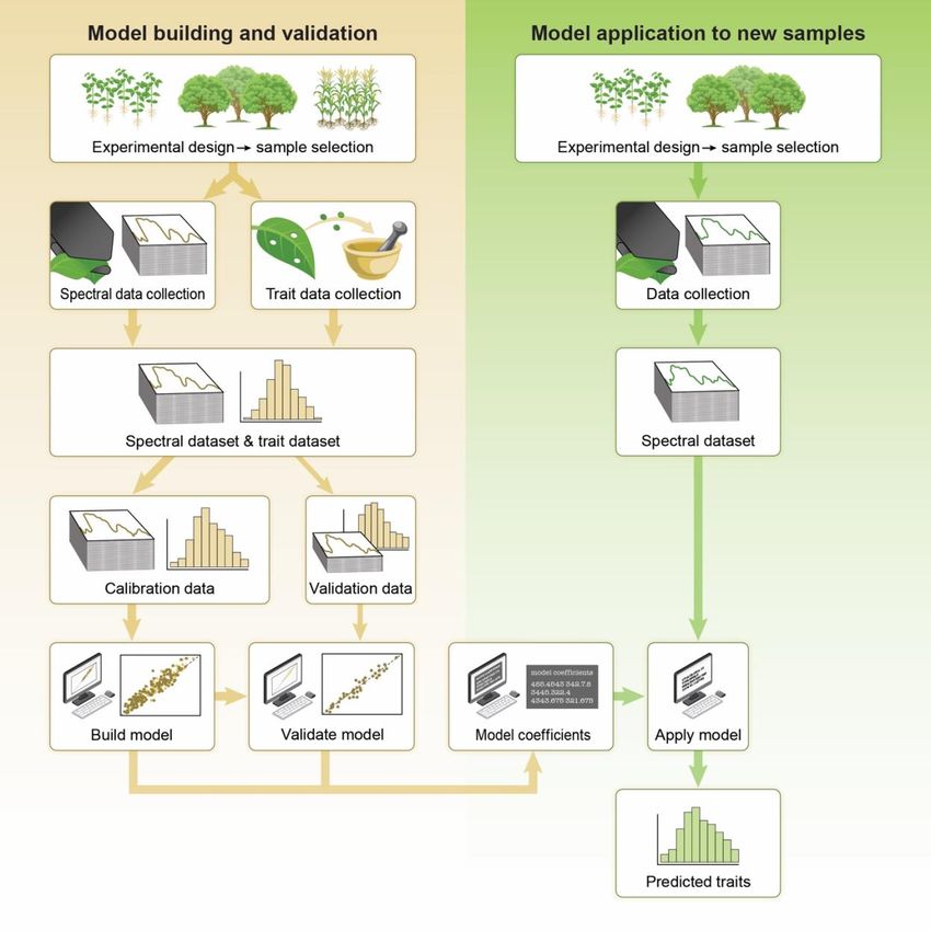
104 Here we present a best-practice “hands-on” guide to perform PLSR modelling for estimating
105 plant traits from leaf-level hyperspectral data, and provide clear guidance on accuracy
106 assessment and model uncertainty. We explain each part of the PLSR workflow from data
107 collection to model building, validation and application (Fig. 1), with key definitions provided in
108 Box 1. We first examine the coordinated data collection of leaf traits and leaf spectra and
109 suggest best practices. We then provide a tutorial guide through an example PLSR modelling
110 scenario accompanied by a detailed, open-source R script. Finally, we discuss common pitfalls
111 when using PLSR and tips for applying PLSR models to novel data. We therefore present a
112 clear and practical guide for readers, reviewers, and researchers; advance knowledge of PLSR
113 and its application; and provide a toolkit for performing one’s own best-practice PLSR.
114
115 Recommendations for collecting leaf spectra and trait data
116
117 In order to build a PLSR model with the best possible predictive power, data collection must be
118 undertaken with the goal of assembling a dataset that captures the potential variation in the
119 plant traits of interest. This involves sampling across the broadest possible trait space and using
120 a spectral collection method that will accurately capture the trait; for some traits timing and
121 temperature are also factors to consider as outlined below. Following Violle et al (2007) we
122 define traits as empirically measured structural, biochemical or physiological properties of
123 leaves; this excludes properties such as Normalized Difference Vegetation Index (NDVI) or
6124 output from a SPAD chlorophyll meter, since it is not meaningful to use leaf reflectance to
125 predict properties that are themselves derived from reflectance within the same wavelength
126 range.
127
128 Collection of leaf trait data
129 Non-linearities in plant traits mean that extrapolation of prediction beyond the range of
130 measured values cannot be considered reliable (Schweiger 2020). Therefore, a measurement
131 plan should be devised to fill the trait space in the calibration data that is anticipated from the
132 combinations of experimental variables under consideration, such as species, leaf age, drought,
133 nutrient treatments and genetic variation (Fig. 2). For the purpose of building a new trait model,
134 this can be achieved by selecting species that are known to have diversity across the target
135 traits, or by manipulating the environment or plants in a way that will result in diversity of the trait
136 of interest.
137
138 The minimum number of paired spectra and measured trait samples required to build a robust
139 model is somewhat dependent on the nature of the trait itself. Enough samples must be
140 collected to provide calibration across the desired data range for predicting traits. Typically,
141 models with good predictive capacity can be built using around 100 samples (Girard et al. 2020;
142 Kleinebecker et al. 2009; Ainsworth et al. 2014; Barnes et al. 2017). However, successful
143 prediction of some traits may require several hundred samples, especially if the data are highly
144 clustered or skewed. Construction of PLSR predictive models with greater than 200 samples is
145 not uncommon (Yendrek et al. 2017; Silva-Perez et al. 2018; Dechant et al. 2017)
146
147 Spectra and trait measurements should generally be made on the same area of leaf material.
148 This principle, and the nature of the trait analysis, will dictate the order in which the spectra and
7149 trait measurements are made. Spectra should be collected prior to any destructive sampling of
150 the leaf material. Special cases for which it is appropriate to measure the spectra after trait
151 collection, or on analogous leaves, are discussed below. Given that spectral measurements
152 represent the area in the leaf sensor field of view, the physical, chemical or physiological traits
153 of interest should also be calculated on an area basis.
154
155 Collection of leaf spectral data
156 A variety of approaches may be used to collect spectral data, including on fresh and dried leaf
157 material. Here we focus on reflectance measurements of fresh leaves using a full range (350–
158 2500 nm) spectroradiometer with a leaf clip or contact probe attachment. The following section
159 describes a basic protocol for measuring leaf-level spectroscopy; refer to Schweiger (2020) for
160 consideration of different instrument types and further protocol details. While we focus on full-
161 range examples, researchers will typically remove data below 450 or 500 nm and greater than
162 2400 nm corresponding with increased sensor noise, and lower signal-to-noise ratio (SNR) and
163 thus potentially adding erroneous information or noise into the PLSR modelling. Moreover, the
164 approaches we present are not specific to this spectral range and the PLSR method is also
165 applicable to datasets with a reduced spectral range, such as within the VNIR (400-1000nm)
166 range. In these cases, however, depending on the trait the PLSR model performance may be
167 reduced because the information provided in the other spectral wavelengths is missing (e.g.
168 Doughty et al. 2011).
169
170 Most off the shelf spectrometer systems that are supplied with a leaf clip or plant probe will also
171 have an internal, calibrated light source. If the researcher plans to use a custom light source it
172 is important to consider any issues related to light intensity and uniformity across the spectral
173 wavelengths of interest, and adjust collection conditions appropriately (e.g. integration time).
8174 However, most spectrometer systems also provide a means for automatic integration that would
175 also adapt to different light sources. This topic is beyond the scope of this work; we refer the
176 reader to Jacquemoud and Ustin. (2019) and expect the data being used has been properly
177 prepared for use with PLSR modelling following their recommendations.
178
179 Ideally, leaves should be measured in situ, or as soon as possible following removal from the
180 plant. Temporary storage in a cool, dark place with appropriate humidity control will minimise
181 metabolic changes in the leaf (Foley et al. 2006; Pérez-Harguindeguy et al. 2013). It is important
182 to ensure that the leaf surface is dry before measuring and that all measurements are made on
183 the same side of each leaf, usually the adaxial surface. Some sample types will require
184 additional preparation before recording spectra, such as creating mats for narrow leaves or
185 needles that will not cover the field of view of the sensor (Kamoske et al., 2021; Noda et al.
186 2013), or measurement of leaf temperature to allow scaling of temperature-sensitive traits
187 (Silva-Perez et al. 2018). It is also assumed that the researcher is familiar with the operation of
188 their specific model of spectrometer and has followed the manufacturer’s guidance on factory
189 calibration, set up and warm up procedures. For a complete treatment of this subject see
190 Jacquemond & Ustin (2019).
191
192 When the sample is ready, calibrate the spectroradiometer using a clean diffuse, 99% (or high
193 reflectivity) reflectance standard. A common option is a LabSphere Spectralon diffuse
194 reflectance standard (Lab Sphere, North Sutton, NH 03260 US). If the researcher would like to
195 convert reflectance from relative reflectance to that corrected by the spectral response of the
196 reflectance standard, it is important to record the serial number of the standard used so that a
197 standard reference correction can be applied. This consists of multiplying each wavelength in
198 the measured spectra by the reference standard calibration coefficient for that wavelength.
9199 200 Once you have selected and recorded the standard, then take three to five measurements of 201 the area to be harvested for trait measurement, avoiding irregular features such as midribs, 202 prominent veins, insect damage or epiphyll cover. In certain plant types, the trait of interest may 203 also influence the section of leaf chosen for analysis. For example, graminoids have well 204 characterised gradients of metabolites along the lamina that should be considered (Pick et al. 205 2011). Care should be taken to minimise the time that the leaf is exposed to the light source to 206 avoid damage from excessive heat. The bottom part of the leaf clip, or the leaf background if 207 using a contact probe, should be optically dark (e.g.
225   measured trait data should be assessed for quality, and erroneous or outlier measurements

226   removed through the use of a standard technique such as boxplot or Cook’s distance before

227   commencing PLSR.

228

229   Special considerations for physiological traits

230   Physiological traits, such as Vc,max, have been derived from reflectance in a wide range of

231   species and growth conditions (Serbin et al. 2012; Yendrek et al. 2017; Silva-Perez et al. 2018;

232   Wu et al. 2019; Meacham-Hensold et al. 2019). When modelling relationships between spectra

233   and physiological traits there are several additional considerations associated with the collection

234   of reflectance data and expression of the physiological trait of interest. Measurement of leaf

235   reflectance can result in damage to the leaf, particularly to sensitive physiological processes, so

236   care must be taken to avoid overheating or over-illuminating the leaf (Serbin et al. 2012). In

237   addition, some physiological traits have a strong temperature sensitivity, and changes in leaf

238   temperature can also impact reflectance (Serbin, 2012; Khan et al., 2021), thus it is important to

239   either minimize heating of leaves during reflectance measurements or to pair leaf temperature

240   measurements close in time with reflectance measurements. Certain physiological

241   measurements can alter the leaf surface, for example when a sealant is used during gas

242   exchange measurements to minimize leakage. The order of measurements will depend on the

243   specific case, with the user considering the traits of interest to determine whether the

244   reflectance measurement might adversely influence the physiological measurement or vice

245   versa. Whilst in an ideal scenario both measurements are made on the same region of the leaf,

246   it is also possible to distribute measurements across the surface of a large leaf, on a different

247   leaflet of a composite leaf, or even on an analogous sample of the same phenological stage and

248   orientation on the plant. Great care should be taken to ensure that equivalent areas or leaves

249   are measured.

                                                                                                          11
250 The scaling of measurements to a reference temperature should also be considered. For
251 example, the predictive power and accuracy of PLSR models have been shown to be greater
252 when the model is built using maximum carboxylation rates that have been normalised to 25°C
253 (Vc,max.25) (Silva-Perez et al. 2018) rather than the Vc,max at measurement temperature, even
254 though both approaches produce successful results (Serbin et al. 2012). This may reflect the
255 covariance between the biochemical and structural properties of the leaf that relate to the
256 investment of resources in Rubisco including known (nitrogen, chlorophyll and LMA) and
257 unknown leaf traits that correlate with Vc,max.25 (Walker et al. 2014; Kattge et al. 2009; Croft et al.
258 2017; Wu et al. 2019). Given the role of environment, especially growth temperature, in
259 determining the investment in Rubisco (Ali et al. 2015; Smith et al. 2019; Kumarathunge et al.
260 2019) and the characteristics of other co-varying leaf traits, it is likely that the success of
261 building PLSR models will be improved when the either the measurement temperature (Vc,max
262 based models) or chosen reference temperature (Vc,max.25 based models) is close to growth
263 temperature. Leaf temperature should be recorded at the time of taking the spectral
264 measurement if it is desired to scale Vc,max to leaf temperature. Leaf temperature data are also
265 required to use spectra to estimate the temperature response of Vc,max. In some cases,
266 physiological parameters have been derived using species-specific kinetic constants (Silva-
267 Perez et al. 2018). We believe that this extra step is not necessary given the intended use of the
268 spectra–trait approach as a screening tool and believe that use of standard kinetic constants
269 (Bernacchi et al. 2001) should be sufficient to develop effective PLSR models. Finally, we note
270 that whilst Vc,max changes with leaf temperature, effects of leaf temperature on the prediction of
271 structural traits such as LMA are small (Khan et al. 2021).
272
273 Special considerations for biochemical traits
274 Biochemical traits comprise another category of leaf traits that may be of particular interest for
275 prediction from spectra. These traits include foliar protein, starch, and chlorophyll content. There
12276 is a long history of using reflectance spectroscopy to detect the concentration of chemical
277 constituents in dried and fresh foliar material in the laboratory, using simple, stepwise, and PLS
278 regression methods (Curran et al. 1992; Martin and Aber 1997; Ustin et al. 1998; Merzlyak et al.
279 2003; R. F. Kokaly et al. 2009; Ely et al. 2019). All such models rely on the basic principle that
280 the depth and magnitude of spectral absorption features associated with molecular bonds
281 should vary in proportion to the concentration of that chemical (R. Kokaly 1999; Curran 1989).
282 For example, N–H bonds, common in proteins, have vibrational absorptions at ~1980 nm and
283 ~2130–2180 nm, with harmonic and overtone frequencies in the NIR and SWIR regions (Curran
284 1989; R. F. Kokaly 2001). Therefore, a model for proteins should rely heavily on the reflectance
285 in these key wavebands (Curran 1989). This should, in theory, make biochemical traits easier to
286 model than structural or physiological traits, as the latter are the consequences of multiple
287 chemical and structural constituents within the sample of interest, and thus direct correlative
288 models are often confounded (Serbin and Townsend 2020).
289
290 A number of considerations still need to be made in order to successfully construct a PLSR
291 model for a biochemical trait. It is prudent to consider both the range and resolution of
292 wavebands measured by the spectroradiometer used for data collection. The wavelength range
293 should be such that the crucial wavebands are measured, and the resolution should be high
294 enough to distinguish bond specific absorption peaks from other peaks of similar bond types
295 (Yoder and Pettigrew-Crosby 1995). Furthermore, it is important to be aware that some
296 chemical types may be masked by absorption associated with other chemicals with a common
297 bond. For example, O–H bonds, the bond type in water, have strong absorption features at
298 ~970, ~1200, ~1400, ~1450 and ~1940 nm (Curran 1989). The O–H bond is also common in
299 cellulose, starch and lignin. Since most fresh plant material is highly water-saturated, a model
300 which leverages the O-H bond absorption features to predict compounds other than water may
301 be confounded if the samples vary in their hydration. In addition, the strong dominance of water
13302 on the SWIR section of the electromagnetic spectrum may mask or obscure other subtle
303 absorption features in the region (Curran, 1989). Drying of sample material will limit the
304 influence of water’s absorption features on spectra, however this is a destructive step that may
305 be impractical for paired spectra and biochemical sampling, which typically relies on flash-
306 freezing samples for subsequent biochemical analysis.
307
308 The time of day of sampling is another consideration, especially for biochemical traits for which
309 the foliar concentration will vary throughout the day as the plant mobilizes and redistributes
310 certain types of biochemical compounds (Nozue and Maloof 2006). For example, sucrose and
311 starch content will be relatively low at dawn but increase over the course of the day, peaking
312 between solar noon and the end of the photoperiod, depending on the species and
313 environmental conditions (Sicher, Kremer, and Harris 1984; Hendrix and Huber 1986). This time
314 of day effect must be accounted for when planning spectral data collection, and can be
315 leveraged to maximize differences in foliar biochemical concentration in order to fill the trait
316 space (Fig. 2).
14317 Tutorial for performing PLSR
318
319 Here we provide general guidelines and typical methods that can be applied to leaf-level PLSR
320 spectra–trait modelling efforts, with regard to data preparation, model development and
321 validation, and interpretation of results. We provide these guidelines in order to improve the
322 robustness of the developed PLSR, but also, critically, to enable easier cross-comparison of
323 published PLSR modelling results across datasets, teams, projects, and biomes. The detailed
324 steps for building a PLSR model will vary for a number of reasons, including the trait of interest,
325 wavelength range of the spectra (e.g. VIS to NIR vs VIS to SWIR), and the goal of the modelling
326 effort; thus it is not possible to provide a single generalised example to cover all applications. To
327 illustrate our suggested approach, we provide the “spectratrait” package, written in the open-
328 source R statistical programming language, which contains examples that utilize publicly
329 available leaf spectra and trait data (Supplemental Table 1) provided through the Ecological
330 Spectral Information System (EcoSIS; https://ecosis.org/). We provide a tutorial (Burnett et al.,
331 2020) to cover what is presented graphically in Fig. 1 through a GitHub repository
332 (https://zenodo.org/record/4730995). The specific example R script summarised here is:
333 “spectra-trait_reseco_lma_plsr_example.R”, with a full illustration of the results available online
334 (https://rpubs.com/sserbin/736861). Users should begin with the README file available in the
335 GitHub repository, which explains the package and illustrative vignettes provided. Before using
336 the code on their own datasets, users should ensure that spectral and trait data have been
337 curated in accordance with the recommendations provided above.
338
339 Data import and preparation
340 While specific to the examples here using EcoSIS datasets, data preparation and import into the
341 chosen statistical modelling environment is a necessary early step (following data quality
15342 control). In the case provided here, we first define the required libraries and other options (Steps
343 1–3), including setting up output directories, prior to data import. Step 4 imports the example
344 dataset from EcoSIS using the EcoSIS application programmer interface (API), using each
345 datasets API key with the “get_ecosis_data.R” function. Steps 5 and 6 show an example of
346 preparing data for fitting and removing missing or bad datasets. This includes the selection of
347 the wavelengths to use in model fitting, in this case 500–2400 nm. Individual researchers should
348 determine the level of data curation and preparation necessary for their specific case, as well as
349 the appropriate wavelengths to use.
350
351 Data transformation
352 Although PLSR does not rely on ‘hard’ distribution assumptions (Sawatsky, Clyde, and Meek
353 2015; Goodhue et al. 2012), better results are obtained when the trait distribution is close to
354 normal or is not significantly skewed. Several methods can be used to inspect the normality of
355 the trait data, including histograms, Q-Q plots, and normality test methods; we use a histogram
356 for illustration in the example code (Step 7). If the histogram does not follow a symmetrical
357 distribution, corresponding transformations should be applied to improve its symmetry before
358 commencing PLSR. For example, a log transformation can be used on data with a long tail on
359 the histogram (i.e. fewer measurements at large trait values). If the value zero occurs in a
360 variable, the fourth root transformation is a good alternative to the logarithm (Wold et al., 2001).
361 While we suggest transforming the trait data if needed, we do not recommend transforming leaf-
362 level spectral data because the reflectance of all wavelengths is collected in the same
363 percentage unit (i.e. 1 – 100%) and the use of a leaf clip minimises environmental interference
364 meaning that transformation to improve the data distribution is not required.
365
366 Data splitting for PLSR calibration and validation
16367 Early PLSR spectra–trait modelling efforts relied solely on internal cross-validation to evaluate
368 model performance (Townsend et al. 2003). More recently, we have instead advocated splitting
369 the full dataset into a model training (calibration) dataset and an out-of-sample validation
370 dataset to provide a more robust and accurate evaluation of prediction, particularly for large
371 datasets (e.g. Serbin et al., 2014). The commonly used cut-offs for calibration vs validation vary
372 between 60% and 80% (Wu et al., 2019; Serbin et al., 2019; Meacham-Hensold et al., 2019). In
373 our example, Step 7 illustrates one way of splitting the data. We use 80% for PLSR calibration
374 in our demonstration (i.e. 80% of the spectra–trait data pairs). Fig. S1 in the example shows the
375 resulting calibration and validation trait distributions based on the split criterion provided. While it
376 is not possible to define all the potential experimental variables that an investigator may use to
377 guide data splitting, such as treatment, species, and spatial range, etc., it is useful to consider
378 one or more key factors that help to define the variation in datasets. For example, ‘species’ is
379 accounted for in our main example, while other examples provided show other variables, such
380 as the NEON (National Science Foundation's National Ecological Observatory Network)
381 example which partitions the data based on an additional variable ‘domain’ corresponding to
382 specific NEON domains (R script: spectra-trait_neon_lma_plsr_example.R). During the splitting
383 procedure the 80/20%, for example, is applied to each bin variable, such as species. Similarly,
384 experimental treatments should also be carefully considered if the number of collections under
385 each treatment or species is significantly different from each other. The ultimate goal of these
386 considerations is to prevent less observed species/domains/treatments from being ignored or
387 under-represented in PLSR calibration.
388
389 Once the data have been split for conducting PLSR, formatting may be needed in order to use
390 the data with the chosen pls package. For example, we illustrate this formatting requirement in
391 Step 8 where we define the PLSR dataset as required by the package. We also show the
392 calibration and validation spectra data side-by-side in Fig. S2.
17393
394 Data permutation to determine the optimal number of components
395 Selecting an optimal number of components (NoC) is critical for the performance of PLSR.
396 Selecting an erroneously small NoC can result in under-fitting of the spectra data and poor
397 model performance. On the other hand, overfitting the model by selecting too many components
398 can yield a model with erroneously high training statistics but will more than likely lead to low
399 model performance, particularly when applied to new observations. This is because overfitting
400 will tend to fit the model to spurious noise in the higher-order components. If there is a lot of
401 error or unexplained variance in the data, or if there is the need to link numerous different
402 observations or data types together (Wolter et al. 2008), modelling can require tens of
403 components. However, our experience is that 20 components is a typical maximum for fitting
404 basic, leaf-level spectra–trait models (Fig. S3). To optimize the process of selecting the NoC we
405 advocate data permutation to identify the optimal NoC and provide the ability to statistically
406 select the smallest necessary to optimize prediction (e.g. Serbin et al., 2014; Ely et al., 2019). In
407 our examples we provide three methods that illustrate ways to permute and select the optimal
408 NoC.
409
410 To perform a data permutation, a sufficient number of PLSR models (20 in our example) need to
411 be built for each of a series of NoC. The averaged predictive performance of these PLSR
412 models is used to determine the optimal NoC. For each model, a subset of samples is randomly
413 selected from the calibration data to train the model, with the rest used for model validation.
414 Here we refer to these as ‘jackknife calibration’ and ‘jackknife validation’ samples to differentiate
415 from the PLSR calibration and validation subsets. Step 10 shows one of the ways to conduct the
416 data permutation. In our example, we used 70% of the calibration subset for jackknife calibration
417 and 30% for jackknife validation, an approach similar to Serbin et al., (2014) or Couture et al.
18418 (2016). Following this, the predicted residual error sum of squares (PRESS) can be calculated
419 for each NoC across all PLSR model ensemble members (Fig. S3). We do not recommend low
420 data splits for jackknife validation, such as 10% (e.g. Asner et al., 2014), as this may lead to
421 overfitting due to an inability to statistically differentiate models with larger numbers of
422 components, particularly with very large calibration datasets.
423
424 Typically, the PRESS plot has a v-shape (decrease then increase) from a low to high NoC and
425 the optimal NoC is indicated by the minimum PRESS (e.g. vertical blue line in Fig. S3).
426 However, this v-shape is not universal. Patterns such as a slowly decreasing PRESS at larger
427 NoC can be obtained when a high variance is present in the spectral data. Despite the
428 decreasing PRESS, ‘overfitting’ may already exist in PLSR with a large NoC, and diminishes the
429 applicability of the model to new datasets. In this case, a threshold can be set to stop the NoC
430 selection at which the change of PRESS becomes insignificant, for example if the change of
431 PRESS from n to n+1 NoC is less than 5%, or a t-test on PRESS does not show significant
432 differences between n and n+1 (p>0.05). In the example code, we demonstrated this with a t-
433 test. Starting from the first NoC, the t-test is conducted between any two consecutive NoC, and
434 stops when the p value is greater than 0.05.
435
436 Final PLSR model calibration and validation
437 Following the selection of the optimal PLSR NoC, a final model should be calibrated using the
438 previously generated calibration data subset. For more detail see the information in the R
439 plsr.out object for PLSR model features; details for parameters can be found in Mevik et al.
440 (2015). In our example, this is shown in Step 11 where we refit the model with the calibration
441 (training) data to define the final model coefficients.
442
19443 Assessment of the final calibration model can be done in two ways. First, leave-one-out cross-
444 validation (LOO-CV), sequential or “venetian blinds” cross-validation can be used to internally
445 assess the model training fit. However, this will likely over-represent the actual model
446 performance. A more appropriate assessment is to utilize the out-of-sample validation dataset
447 as validation of the model performance. This approach is generally effective when both the
448 calibration and validation data are representative of the trait space. For example, we show the
449 assessment of the LMA model using our withheld validation data across increasing PLSR model
450 components up to the final optimal number, 11 (Fig. S4). We show both how the root mean
451 square error of prediction (RMSEP) decreases and how the coefficient of determination (R 2)
452 increases with successive components to a final RMSEP of 11.7 g m -2 and R2 of 0.86. It is,
453 however, important to note that over-estimation of model performance is still a potential issue in
454 our proposed approach as the calibration and validation subsets are not fully independent.
455 Additional steps may be considered to reaffirm the performance of the final PLSR. For example,
456 an extra independent dataset can be used to avoid model over-estimation and also test its
457 generality to new observations. While this could seem unnecessary, often the overall goal of
458 PLSR modelling is to develop models that can be used to estimate traits for new samples (e.g.
459 Serbin et al., 2019) so this additional step may be important in some cases.
460
461 As we show in Fig. 4, there are various metrics to assess model performance. These include
462 the R2, RMSEP, and the percent RMSEP (RMSEP as a percentage of the trait range). In Step
463 12 of our example, we further illustrate a way to evaluate model fit through both calibration and
464 validation fit statistics and assessment of residuals. For example, Fig. S5 provides a side-by-
465 side assessment of the LMA model performance for the calibration and validation of this model
466 using the withheld dataset. The calibration and validation residual plots are provided to help
467 visually assess any significant bias or skewness in the model fit. For example, when reviewing
468 the residuals, if a strong non-linear trend is found it may indicate that data transformation (e.g.
20469 square root transform, Serbin et al., 2019) may be required. In this specific example we see that
470 the model R2 is similar for the calibration and validation results, while the RMSEP increased
471 slightly for the validation data, from 12.84 to 13.68 g m -2.
472
473 An additional step that is often useful for assessing PLSR models is to explore the final model
474 coefficients and VIPs (Fig. S6), and this is shown in Step 13 in the tutorial example. In this case
475 we plot the final eleven-component PLSR regression coefficients and the VIPs across the same
476 wavelength range. Here we see that the areas of highest contribution to the estimation of LMA
477 in this dataset tend to occur in the visible wavelengths, followed by portions of the SWIR
478 regions, with a slightly lower contribution from the NIR bands. We can also see that the resulting
479 coefficient plot shows reasonably smooth values across most of the spectrum, with some areas
480 that have a higher-frequency variation related to regions of spectrometer detector overlap where
481 the signal-to-noise is often lower, or other features that may be related to measurement
482 artifacts. The coefficient plot can also be used to identify spectral features related to specific
483 constituents. Known spectral peaks can be retrieved and used to give a possible explanation of
484 why the model successfully predicts the trait of interest (Dechant et al. 2017). Typically, a high-
485 degree of high-frequency variation in a coefficient plot may indicate an overfit model (Asner et
486 al. 2014).
487
488 PLSR model uncertainty analysis
489 In our example we have illustrated how to prepare, define optimal components, fit, and evaluate
490 a PLSR model using cross-validation, permutation analysis and independent validation.
491 However, it may be of interest for researchers to understand the inherent uncertainties in their
492 model when predicting new values based on leaf spectra. This can be achieved by deriving
493 model predictive uncertainty via a permutation analysis (Serbin et al. 2014; Couture et al. 2016;
494 Ely et al. 2019; Wu et al. 2019). Most commonly this is done by: 1) generating PLSR ensembles
21495 through permutation e.g. jackknife or bootstrapping, 2) collating these results into a matrix of
496 possible models, 3) applying the ensembles to new observations to derive a distribution of fitted
497 values for each observation, and then 4) summarizing the fit uncertainty given the variance
498 around each estimated value. In addition, once the model ensembles are generated they may
499 be used with the original final model to estimate new trait values and the uncertainties around
500 these estimates using the permuted model coefficients (e.g. Serbin et al., 2019).
501
502 There are various ways to conduct permutation analysis (Schweiger et al. 2018; Couture et al.
503 2016; Singh et al. 2015), but in this case we followed a basic jackknifing approach. Step 14 in
504 our example illustrates the internal jackknife feature of the R PLS package, which we used to
505 develop the PLSR model ensembles for the uncertainty assessment. The resulting jackknife
506 coefficients are shown in Fig. S7. As expected, the general shape of the jackknife coefficients
507 across the spectral range is similar to the full model (Figure S6), but also shows the variance in
508 coefficients related to the resampling of the full calibration data that is used to quantify and
509 represent the uncertainty of the PLSR model. Using the full model and jackknife coefficients, we
510 then provide the mean estimate as well as both the 95% confidence and prediction intervals of
511 the estimated LMA values in the validation dataset. We show the estimated uncertainty in Fig.
512 S8, which shows the standard observed vs predicted presentation of the results, with R 2,
513 RMSEP and %RMSEP, as well as the prediction interval around each validation data point. This
514 is similar to that provided by previous studies (Couture et al. 2016; Ely et al. 2019; Wu et al.
515 2019) and is a recommended way to present overall model predictive performance in a scientific
516 paper.
517
518
519
22520 Final steps
521 After fitting the model and estimating the inherent uncertainty, the last step is to output or save
522 the model, fit statistics, diagnostics, final model coefficients, and permutation coefficients.
523 Importantly, the model coefficients and permutation coefficients represent the resulting model
524 and the resulting model with uncertainties, respectively. These coefficients are the main
525 features used to estimate traits from new leaf spectral observations. We illustrate saving PLSR
526 results in Steps 15 and 16 in the example.
23527 Common pitfalls using PLSR when predicting plant traits
528
529 In this article we have highlighted the uses and applications of PLSR modelling in the context of
530 estimating leaf traits with high-resolution leaf-level spectroscopy data. While this method has
531 proved useful in a range of applications from forestry, agriculture, plant biology, and remote
532 sensing, it is not the only method available—and is not always the best method—for building
533 links between plant functional properties and remote sensing signatures. For example PLSR
534 can suffer from a strong influence from outliers, even if the fraction of erroneous or otherwise
535 questionable data is small relative to the total number of observations (Wold et al. 2001).
536 Moreover, as stated here and elsewhere (Schweiger 2020), PLSR, like all empirical methods,
537 requires that the training dataset encompass the range of expected values for a trait to which
538 the model will be applied otherwise it will likely underperform at the extremes of the distribution
539 (Fig. 2). As such, it is recommended that researchers who wish to develop models for
540 operational applications, or across diverse vegetation, focus on building large datasets that
541 cover the trait space they expect (e.g. Serbin et al. 2019). This, however, can present a
542 significant challenge as the cost and effort to develop a model for any one location or
543 experiment can be large when factoring in logistical costs for data collection. Therefore, we
544 recommend that datasets such as those available from EcoSIS be leveraged whenever possible
545 to expand the training dataset to encompass more expected variation in spectra and trait
546 observations. Past efforts suggest this is possible (e.g. Serbin et al 2019) but additional
547 research into the ease of combining trait and spectral collection methods, instruments, and
548 other conditions is still required to fully understand the generality of PLSR approaches across
549 large and diverse datasets. Furthermore, other issues can impact the performance of PLSR
550 modelling such as noisy spectral data, particularly in the regions of known absorption features of
24551 certain traits such as the SWIR region; this is common with the use of some foreoptics such as 552 integrating spheres (e.g. Yang et al., 2016). 553 554 Another pitfall of PLSR modelling is the potential to overfit the training data. PLSR modelling 555 depends on the decomposition of the original data into a number of orthogonal axes equal to the 556 number of different components selected in the modelling step. This is a critical step to develop 557 the fewest number of different rotations or orthogonal axes needed to optimally model the 558 dependent variable(s) [Y] using the predictor matrix [X]. This makes this method more suitable 559 than linear regressions by reducing the number of variables used in the model. However, in this 560 step it is possible to overfit the PLSR model if too many components are chosen. In that case, 561 the model will start to use the noise as if it were structural information to explain the variation in 562 Y. This effect is similar to trying to fit a linear model with as many parameters as the number of 563 observations. In that case the model will describe exactly the observation but the parameters 564 will not be significant. When this happens, it is possible to over-train the model with a very large 565 number of components. The more components included in the model the more likely spurious 566 noise is included. For most plant traits
576   measurements and for reducing the risk of overfitting. However, the way in which PLSR is

577   carried out and the choice of the number of components is of paramount importance. Therefore,

578   the chosen method should always be carefully described, and the number of components

579   should be as parsimonious as possible so other researchers can use the model with new data

580   while having the same predictive power. The use of a validation dataset to evaluate PLSR is

581   also very important for reducing the risk of overestimating the quality of the model. The Root

582   Mean Square Error of Prediction (RMSEP) and correlation (R 2) are the recommended indicators

583   of performance and should both be reported. %RMSEP is useful for facilitating comparisons

584   between traits for which the data ranges span different scales. Fig. 5 provides an example of a

585   figure and legend to report the performance of a PLSR model. Model reporting should also

586   include the number of points of the validation dataset (n) and the NoC. Other metrics and

587   figures could also be added if needed such as the Mean Absolute Error (MAE) which is less

588   sensitive to outliers than the RMSEP. The histogram of the residuals can be also interesting to

589   report as it contains information on the outliers and under- versus over-prediction. (The code to

590   produce those figures is provided in the GitHub repository.) However, we suggest always using

591   the RMSEP and R2 as a minimal basis for all PLSR descriptions to allow direct comparison

592   between models.

593

594   In order for other researchers to utilize an existing PLSR model with new datasets, the

595   coefficients of the PLSR model, the intercept, and any transformations of the variable should

596   also be published. For example, GitHub (e.g.

597   https://github.com/serbinsh/SSerbin_etal_2019_NewPhytologist/releases/tag/1.2.1) or the

598   Ecological Spectral Model Library (EcoSML.org) model aggregator portal can be used to

599   provide access to the final PLSR models.

600

                                                                                                       26
601 With the information reported above, potential users can determine if an existing model is
602 suitable for their research needs. However, special consideration is needed to determine if the
603 PLSR model can be applied in their environment and for their specific samples. First, it is
604 always a good practice to assess the quality of the model using at least 20 new samples.
605 Second, it is important to note that the models should be applied using the same protocol and
606 the same type of equipment as used in the original model development. An attractive use of
607 leaf-level PLSR models would be to apply them on a larger scale using other sensors such as
608 multispectral or hyperspectral cameras that can be deployed in unoccupied aerial systems,
609 aircraft or satellite platforms. Such an aim is not straightforward, mainly because the 3D position
610 of the leaves and their light environment are not uniform between samples as they are for
611 proximal spectral data collection and this means that these aspects must be accounted for when
612 developing a canopy model. In addition, sensor characteristics such as the bandwidth and
613 number of wavebands may vary between instruments. As a consequence, the application of a
614 PLSR model built at the leaf scale to canopy spectral data can lead to a significant bias (Al
615 Makdessi et al. 2019). Instead, the structure of a canopy and sensor characteristics must be
616 accounted for when building a PLSR model. In practice, this means that such a model should be
617 built and applied at the canopy scale, rather than building a leaf-level model and applying it at
618 the canopy scale (e.g. Burnett et al., 2021). A detailed discussion of these points is outside the
619 scope of this manuscript, although for the interested reader we provide an example of a canopy
620 scale application of our approach using a dedicated model (Supplementary Table 1). Lastly, the
621 PLSR model should not be applied on new samples outside the range of the original dataset
622 used to calibrate the PLSR model (Figure 2b).
623
624 In conclusion, this practical guide to PLSR models will enable researchers to better understand
625 and use this powerful technique for predicting leaf traits from leaf-level spectral data—both for
626 building new spectra–trait models and applying existing models to new spectral data. The
27627 detailed tutorial examples can be used as a guide to achieving optimal results when building
628 new models, which will in turn, facilitate a higher degree of confidence in applying these or other
629 published models to new spectral datasets, and leveraging existing datasets to examine leaf
630 traits.
28631 Supplementary Information
632 Supplementary Table 1. Details of the R scripts provided in our GitHub repository.
633 Supplementary Protocol S1. Illustration of our PLSR tutorial.
634 Supplementary Protocol S2. A compressed zip file containing the ‘spectratrait’ R package
635 (spectratrait-v1.0.4.zip).
636 Supplementary Protocol S2 contents. Pdf file detailing the contents of the zipped
637 supplementary R package (zip_package_contents.pdf).
638
639 Supplementary figures referenced in the manuscript are included in the vignette and as outputs
640 of the R script.
641
642 Acknowledgements
643 This work was supported by the Next-Generation Ecosystem Experiments (NGEE Arctic and
644 NGEE Tropics) projects that are supported by the Office of Biological and Environmental
645 Research in the Department of Energy, Office of Science, and through the United States
646 Department of Energy contract No. DE-SC0012704 to Brookhaven National Laboratory. The
647 authors thank Tiffany Bowman of Brookhaven National Laboratory for graphic design work (Fig.
648 1).
649
650 Author contributions
651 ACB, AR and SPS conceived the manuscript. ACB led the preparation of the manuscript. All
652 authors contributed to the writing of the manuscript. The R script was developed by SPS with
653 significant contributions from JA and JL and additional contributions from all authors.
654
655 Protocol DOI
656 The R script developed to accompany this manuscript, along with a readme file and illustrative
657 vignettes, are located in a GitHub repository. A link to our repository has been uploaded as a
658 protocol on protocols.io (Burnett et al., 2020) and may be viewed using the following DOI:
659 dx.doi.org/10.17504/protocols.io.bmhek33e
660
661 Data availability statement
662 All illustrative examples in this study use published, open-source data which are available online
663 through the Ecological Spectral Information System (EcoSIS, https://ecosis.org/) as outlined
664 within the manuscript and Supplemental Table 1.
29References
Ainsworth EA, Serbin SP, Skoneczka JA, and Townsend PA. 2014. Using leaf optical properties to
detect ozone effects on foliar biochemistry. Photosynthesis Research 119 (1-2): 65–76.
Ali AA, Xu C, Rogers A, McDowell NG, Medlyn BE, Fisher RA, Wullschleger SD, et al. 2015. Global-
scale environmental control of plant photosynthetic capacity. Ecological Applications 25 (8):
2349–65.
Al Makdessi N, Ecarnot M, Roumet P, and Rabatel G. 2019. A spectral correction method for multi-
scattering effects in close range hyperspectral imagery of vegetation scenes: application to
nitrogen content assessment in wheat. Precision Agriculture 20: 237-259.
https://doi.org/10.1007/s11119-018-9613-2.
Asner G. 2008. Hyperspectral remote sensing of canopy chemistry, physiology, and biodiversity in
tropical rainforests. Hyperspectral Remote Sensing of Tropical and Sub-Tropical Forests.
https://doi.org/10.1201/9781420053432.ch12.
Asner GP, Martin RE, Carranza-Jiménez L, Sinca F, Tupayachi R, Anderson CB, and Martinez P.
2014. Functional and biological diversity of foliar spectra in tree canopies throughout the Andes
to Amazon region. New Phytologist 204 (1): 127–39.
Barnes ML, Breshears DD, Law DJ, van Leeuwen WJD, Monson RK, Fojtik AC, Barron-Gafford GA,
and Moore DJP. 2017. Beyond greenness: detecting temporal changes in photosynthetic
capacity with hyperspectral reflectance data. PloS One 12 (12): e0189539.
Bernacchi CJ, Singsaas EL, Pimentel C, Portis Jr AR, and Long SP. 2001. Improved temperature
response functions for models of Rubisco-limited photosynthesis. Plant, Cell and Environment
24 (2): 253-259. https://doi.org/10.1111/j.1365-3040.2001.00668.x.
Bjorkman AD, Myers-Smith IH, Elmendorf SC, et al. 2018. Plant functional trait change across a
warming tundra biome. Nature 562: 57-62.
Burnett, AC, Anderson, J, Davidson, KJ, Ely, KS, Lamour, J, Li, Q, Morrison, B, Yang, D, Rogers, A,
Serbin, SP. 2020. Example PLSR for Predicting Leaf Traits from Leaf Spectra. protocols.io
https://dx.doi.org/10.17504/protocols.io.bmhek33e
Burnett AC, Serbin SP, Rogers A. 2021. Source:sink imbalance detected with leaf and canopy‐level
spectroscopy in a field‐grown crop. Plant, Cell and Environment
https://doi.org/10.1111/pce.14056
Cornelissen JHC, Lavorel S, Garnier E, Díaz S, Buchmann N, Gurvich DE, Reich PB, et al. 2003. A
handbook of protocols for standardised and easy measurement of plant functional traits
worldwide. Australian Journal of Botany 51 (4): 335-380. https://doi.org/10.1071/bt02124.
Couture JJ, Singh A, Rubert‐Nason KF, Serbin SP, Lindroth RL, and Townsend PA. 2016.
Spectroscopic determination of ecologically relevant plant secondary metabolites. Methods in
Ecology and Evolution 7 (11): 1402-12. https://doi.org/10.1111/2041-210x.12596.
Croft H, Chen JM, Luo X, Bartlett P, Chen B, and Staebler RM. 2017. Leaf chlorophyll content as a
proxy for leaf photosynthetic capacity. Global Change Biology 23 (9): 3513–24.
Curran PJ. 1989. Remote sensing of foliar chemistry. Remote Sensing of Environment 30 (3): 271-
278. https://doi.org/10.1016/0034-4257(89)90069-2.
Curran PJ, Dungan JL, Macler BA, Plummer SE, and Peterson DL. 1992. Reflectance spectroscopy
of fresh whole leaves for the estimation of chemical concentration. Remote Sensing of
Environment 39 (2): 153-166. https://doi.org/10.1016/0034-4257(92)90133-5.
Dechant B, Cuntz M, Vohland M, Schulz E, and Doktor D. 2017. Estimation of photosynthesis traits
from leaf reflectance spectra: Correlation to nitrogen content as the dominant mechanism.
Remote Sensing of Environment 196: 279-292. https://doi.org/10.1016/j.rse.2017.05.019.
Doughty C, Asner G, and Martin R. 2011. Predicting tropical plant physiology from leaf and
canopy spectroscopy. Oecologia 165:289-299
30You can also read