Optimizing towing processes at airports - Jia Yan Du - mediaTUM
←
→
Page content transcription
If your browser does not render page correctly, please read the page content below
Optimizing towing
processes at airports

              Jia Yan Du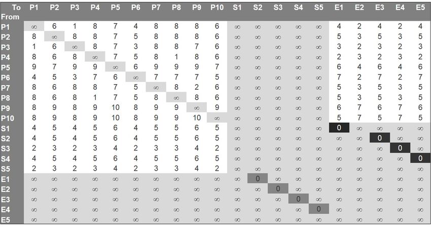
TECHNISCHE UNIVERSITÄT MÜNCHEN

       FAKULTÄT FÜR WIRTSCHAFTSWISSENSCHAFTEN -
         LEHRSTUHL FÜR OPERATIONS MANAGEMENT

             Optimizing towing
            processes at airports

                       Dipl.-Kffr. Univ. Jia Yan Du

Vollständiger Abdruck der von der Fakultät für Wirtschaftswissenschaften
der Technischen Universität München zur Erlangung des akademischen
Grades eines

              Doktors der Wirtschaftswissenschaften
                              (Dr. rer. pol.)

genehmigten Dissertation.

        Vorsitzender: Univ.-Prof. Dr. Martin Grunow
        Prüfer der Dissertation:
        1. Univ.-Prof. Dr. Rainer Kolisch
        2. Univ.-Prof. Dr. Jens O. Brunner, Universität Augsburg

Die Dissertation wurde am 19.12.2013 bei der Technischen Universität
München eingereicht und durch die Fakultät für Wirtschaftswissenschaften
am 15.03.2014 angenommen.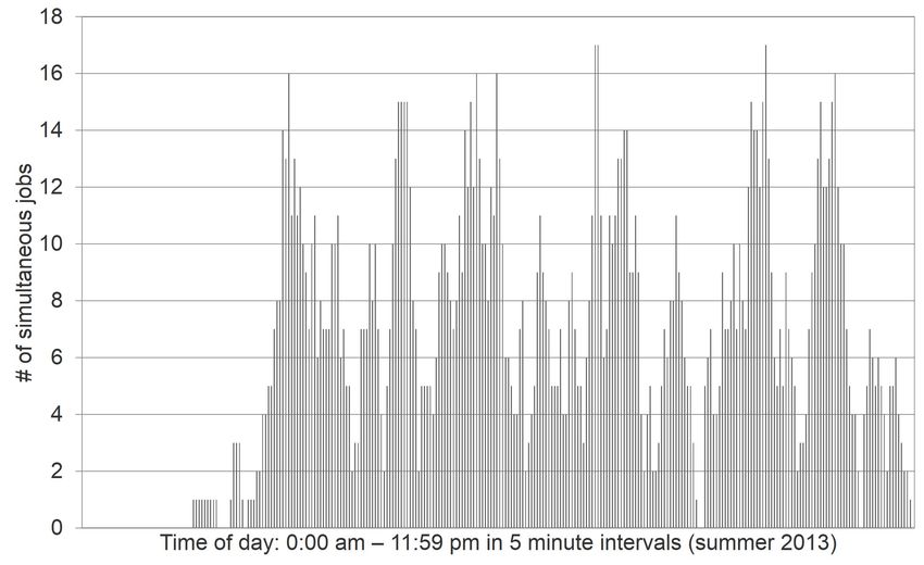
Contents

Table of Contents                                                                               i

List of Tables                                                                                 iii

List of Figures                                                                                iv

1 Introduction                                                                                  1
  1.1 Towing processes at airports . . . . . . . . . . . . . . . . . .                          1
  1.2 Structure of the thesis . . . . . . . . . . . . . . . . . . . . .                         3

2 Scheduling of towing processes                                                                5
  2.1 Related literature . . . . . . . . . .   . . . . .   .   .   .   .   .   .   .   .   .    5
      2.1.1 Literature on push-back . .        . . . . .   .   .   .   .   .   .   .   .   .    6
      2.1.2 Literature on vehicle routing      problem     .   .   .   .   .   .   .   .   .    7
  2.2 Mathematical model . . . . . . . .       . . . . .   .   .   .   .   .   .   .   .   .   10
      2.2.1 Depot model . . . . . . . .        . . . . .   .   .   .   .   .   .   .   .   .   11
      2.2.2 Tractor model . . . . . . . .      . . . . .   .   .   .   .   .   .   .   .   .   16
  2.3 Column generation heuristic . . . .      . . . . .   .   .   .   .   .   .   .   .   .   20
  2.4 Computational study . . . . . . . .      . . . . .   .   .   .   .   .   .   .   .   .   24
  2.5 Case study . . . . . . . . . . . . . .   . . . . .   .   .   .   .   .   .   .   .   .   28
  2.6 Summary . . . . . . . . . . . . . .      . . . . .   .   .   .   .   .   .   .   .   .   31

3 Fleet composition of towing tractors                                                         33
  3.1 Related literature . . . . . . . . . . . . . . . . . . . . . . . .                       34
  3.2 Mathematical formulation and solution approach . . . . . .                               36
  3.3 Demand and fleet related input data . . . . . . . . . . . . .                            44

                                      i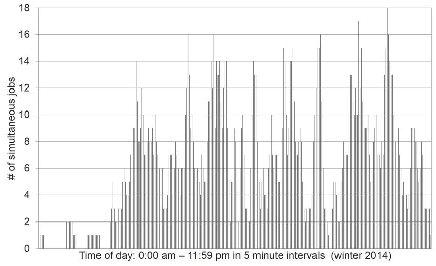
3.3.1 Demand pattern generation          . . .   .   .   .   .   .   .   .   .   .   .   .   44
         3.3.2 Demand forecasting . . . . .       . . .   .   .   .   .   .   .   .   .   .   .   .   46
         3.3.3 Consideration of the existing      fleet   .   .   .   .   .   .   .   .   .   .   .   50
   3.4   Case study . . . . . . . . . . . . . .   . . .   .   .   .   .   .   .   .   .   .   .   .   50
         3.4.1 Basic scenario . . . . . . . .     . . .   .   .   .   .   .   .   .   .   .   .   .   51
         3.4.2 Demand and risk scenarios .        . . .   .   .   .   .   .   .   .   .   .   .   .   54
         3.4.3 Cost scenarios . . . . . . . .     . . .   .   .   .   .   .   .   .   .   .   .   .   56
         3.4.4 Fleet management scenarios         . . .   .   .   .   .   .   .   .   .   .   .   .   59
         3.4.5 Green field scenario . . . . .     . . .   .   .   .   .   .   .   .   .   .   .   .   59
   3.5   Summary . . . . . . . . . . . . . .      . . .   .   .   .   .   .   .   .   .   .   .   .   61

4 Conclusion                                                                                          62
  4.1 Implications for towing service providers . . . . . . . . . . .                                 62
  4.2 Contributions of this work . . . . . . . . . . . . . . . . . . .                                63
  4.3 Directions for future research . . . . . . . . . . . . . . . . .                                64

A Tractor model - MP and SP                                                                           66

B Computational test results - CGH depot model vs. CGH
  tractor model                                        70

C Fleet composition model - MIP                                                                       71

D Abbreviations and notations                                                                         74
  D.1 General abbreviations . . . . . . . . . . . . . . .                 .   .   .   .   .   .   .   74
  D.2 Notations depot model - MIP . . . . . . . . . .                     .   .   .   .   .   .   .   76
  D.3 Notations tractor model - MIP . . . . . . . . . .                   .   .   .   .   .   .   .   77
  D.4 Notations depot model - MP and SP . . . . . .                       .   .   .   .   .   .   .   79
  D.5 Notations fleet composition model - MP and SP                       .   .   .   .   .   .   .   81

Bibliography                                                                                          83

                                      ii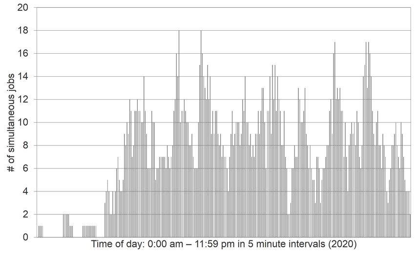
List of Tables

 2.1   Computational test results - Heterogeneous fleet, 10 planes .         25
 2.2   Computational test results - Homogeneous fleet, 10 planes .           26
 2.3   Computational test results - Heterogeneous fleet, 25/50 planes        27
 2.4   Case study results - Variable costs and time . . . . . . . . .        29
 2.5   Case study results - Tractors . . . . . . . . . . . . . . . . . .     29

 3.1   Example investment plan a for tractor type b . . . . . . .    .   .   43
 3.2   Procedure for demand pattern generation . . . . . . . . .     .   .   44
 3.3   Step 4 - Compatibility structure case 1 . . . . . . . . . .   .   .   46
 3.4   Step 4 - Compatibility structure case 2 . . . . . . . . . .   .   .   46
 3.5   Step 4 - Compatibility structure case 3 . . . . . . . . . .   .   .   47
 3.6   Forecasting of numbers of towing jobs per day . . . . . .     .   .   47
 3.7   Parameter settings and input data for the basic scenario      .   .   51

 B.1 Computational test results CGH depot model vs. CGH trac-
     tor model - Heterogeneous fleet of 23 tractors and 12 types,
     10/25 planes . . . . . . . . . . . . . . . . . . . . . . . . . . .      70

                                   iii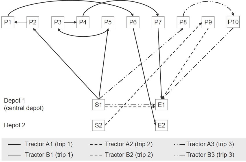
List of Figures
1.1 Operational and strategic planning problem of towing pro-
cesses at airports . . . . . . . . . . . . . . . . . . . . . . . . 3
2.1 Depot structure (example) . . . . . . . . . . . . . . . . . . . 11
2.2 Output of depot model (example) . . . . . . . . . . . . . . . 12
2.3 Travel time matrix (example for depot model) . . . . . . . . 13
2.4 Output of tractor model (example) . . . . . . . . . . . . . . 17
2.5 Development of the lower bound per iteration of problem
instance 19 . . . . . . . . . . . . . . . . . . . . . . . . . . . 28
2.6 SP runtime per iteration of problem instance 19 . . . . . . . 28
2.7 Overview travel time per tractor . . . . . . . . . . . . . . . . 30
3.1 Step 2 and step 3 - Tractor occupancy time per job and max-
imum number of simultaneous jobs . . . . . . . . . . . . . . 45
3.2 Temporal distribution of jobs (summer 2013) . . . . . . . . . 48
3.3 Temporal distribution of jobs (winter 2014) . . . . . . . . . . 48
3.4 Temporal distribution of jobs (2020) . . . . . . . . . . . . . 49
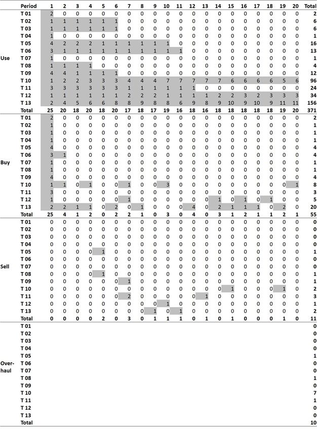
3.5 Number of tractors used, bought, sold and overhauled per
period and tractor type (basic scenario) . . . . . . . . . . . . 52
3.6 Number of tractors bought and sold per period (basic scenario) 53
3.7 Number of tractors used per period and tractor type (basic
scenario) . . . . . . . . . . . . . . . . . . . . . . . . . . . . . 53
3.8 Number of tractors used per period and categories of ”exist-
ing” vs. ”new” (basic scenario) . . . . . . . . . . . . . . . . 54
3.9 Waiting time scenarios vs. basic scenario . . . . . . . . . . . 55
3.10 Demand scenarios vs. basic scenario . . . . . . . . . . . . . . 55
iv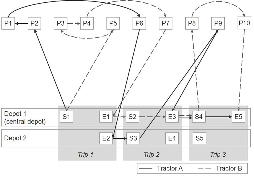
3.11   Delta of D-10% scenario and basic scenario . . . . . . . . . .        56
3.12   Selling price scenarios vs. basic scenario . . . . . . . . . . .      57
3.13   Overhaul cost scenarios vs. basic scenario . . . . . . . . . .        58
3.14   Utilization scenarios vs. basic scenario . . . . . . . . . . . .      58
3.15   Fleet management scenarios vs. basic scenario . . . . . . . .         59
3.16   Green field scenario vs. basic scenario . . . . . . . . . . . . .     60
3.17   Number of tractors used per period and tractor type (green
       field scenario) . . . . . . . . . . . . . . . . . . . . . . . . . .   60

                                     v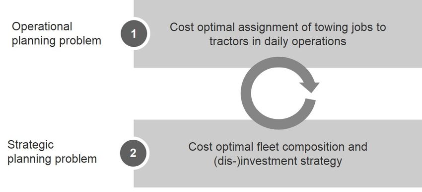
Chapter 1

Introduction

The number of aircraft movements is expected to increase by 50% in Europe
from 2012 to 2035. The capacity at airports will be the bottleneck limiting
future growth. Up to 12% of the demand in 2035 will not be satisfied (see
EUROCONTROL [34]). Airports face the challenge of improving efficiency
in order to cope with increasing demand while fully exploiting available
resources. In the recent past, capacity constraints and cost pressure tight-
ened flight schedules. This threatens smooth operations and punctuality. A
primary source of delays are disruptions in the turnaround process. Accord-
ing to EUROCONTROL [33] the turnaround process accounted for 36% of
delays at European airports in 2011. This work is dedicated to towing ac-
tivities as one of the major steps in the turnaround process. This chapter
introduces the towing process and the operational and strategic planning
problem of towing service providers. Finally, it lays out the structure of the
thesis.

1.1     Towing processes at airports
Planes do not have a reverse gear, so they need assistance to leave the park-
ing position. They can use their own engines to move forward on the ground.
However, over long distances towing is often more economical and ecological
(see Airport Authority Zürich Airport [2]). Towing is distinguished between
push-back, repositioning and maintenance towing.

• Push-back. The plane with the passengers (or cargo) on board is pushed
  backwards from its parking position (e.g. the gate) to the taxiway. From

                                      1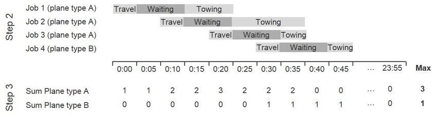
1.1 Towing processes at airports                                            2

  there the plane can move on its own to the runway for take off.
• Repositioning. The empty plane is towed from one parking position
  to another. For instance, a repositioning takes place if an occupied gate
  must be used by an incoming flight. Normally, the blocking plane has
  ample time before departure.
• Maintenance towing. The empty plane is towed to the hangar area for
  maintenance or repairs.

There are two main categories of tractors to carry out the jobs: tractors
with and without a towbar. Towbar tractors connect with the plane via a
towbar. Towless tractors raise the front part of a plane and position it on
the tractor itself (see Kazda and Caves [40]). The largest towless tractor
currently on the market is the Goldhofer AST 1X. Equipped with two 680
horsepower diesel engines, the tractor is capable of towing the 560-tonne
A380 (see Goldhofer AG [36]). Towbar tractors usually are more flexible
with respect to compatibility with plane types and have lower maintenance
and investment costs compared to towless tractors. However, each plane
type requires a different tow bar. Therefore, towbar tractors must return
to a depot to change the towbar between two jobs in case of different plane
types. Furthermore, a second person (e.g. the pilot) must be present in the
cockpit while the plane is towed by a towbar tractor.
    In this thesis I investigate the optimization of towing processes taking
the perspective of a towing service provider. Operating costs as well as
investment costs of towing tractors are high. Investment costs can reach
around 1 million Euro per tractor (see Deutsche Lufthansa AG [27]). A
towing service provider faces two key questions (see Figure 1.1):
    1. Operational planning problem: What is the cost optimal
assignment of towing jobs to towing tractors in daily operations?
The towing service provider is responsible for carrying out all towing jobs
on time. The assignment of tractors to towing jobs is part of their daily
operations. Today most towing service providers apply manual planning
tools, often resulting in inefficient schedules. The assignment significantly
impacts service quality, as well as operating costs. In the short-term the
available fleet for the assignment is given by the existing tractors.
    2. Strategic planning problem: What is the cost optimal fleet
composition and respective (dis-)investment strategy? On a strate-
gic level the towing service provider is responsible for deciding on the fleet
size and mix and thereby determining in each period how many tractors are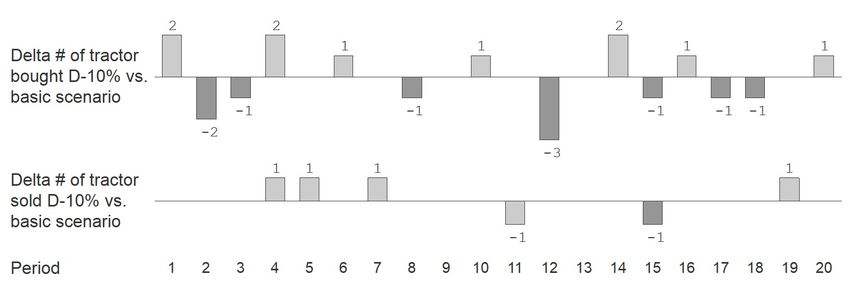
1.2 Structure of the thesis                                               3

Figure 1.1: Operational and strategic planning problem of towing processes
            at airports

to be bought, overhauled or sold. This decision impacts investment costs,
operating costs, as well as the service level.
    Both planning problems are interlinked. An optimized tractor fleet,
which can be influenced by tackling the strategic planning problem, allows
for more efficient schedules in daily assignments. An efficient assignment,
which is addressed in the operational planning problem, can reduce the num-
ber of tractors required, i.e. impacts the fleet size. Hence, both problems
need to be examined in order to optimize towing processes from a holistic
perspective. This thesis addresses both the operational and the strategic
planning problem of towing processes at airports.

1.2     Structure of the thesis
The thesis contains four chapters. Chapter 1 introduces towing processes at
airports, the related planning problems and the structure of the thesis. The
two core chapters address the planning of towing processes from an opera-
tional perspective (Chapter 2) and from a strategic perspective (Chapter 3).
Chapter 2 introduces a vehicle routing based scheduling model. I present
a column generation heuristic as solution procedure and examine its per-
formance in a computational study. A case study demonstrates how the
model can be applied as a tool for identifying cost drivers and evaluating
the efficiency of manual schedules in retrospect. The case study aims to
1.2 Structure of the thesis 4 derive insights which support schedulers in their future work. This chapter is based on Du et al. [30]. Chapter 3 addresses the problem of a cost mini- mal fleet composition. A model is introduced which supports towing service providers in their strategic investment decision. In a case study, a multi- period fleet (dis-)investment plan is derived for a towing service provider at a major European airport. Furthermore, a 4-step approach to aggre- gate demand based on flight schedule information is presented. In several scenarios I analyze the impact of demand, flight schedule disruptions and cost structures on the optimal fleet and conclude on the robustness of the investment plan with respect to these factors. This chapter is based on Du et al. [29]. The work concludes with the main findings and a discussion on potential directions for future research in Chapter 4.
Chapter 2

Scheduling of towing processes

In this chapter, I introduce a model that assigns tractors to towing jobs
in order to minimize costs from perspective of a towing service provider.
The assignment is subject to various operational restrictions and airport
dependent specifications. For instance, technical compatibility with plane
types and specific variable costs are associated with different tractor types.
Furthermore, the time window to start the push-back is linked to the plane
departure time, i.e. the service must take place during a fixed time window.
Penalty costs occur if the push-back is delayed. Multiple depots to which
tractor drivers can return for work breaks are considered. This implicates
multiple uses of tractors in one planning period.
    The remainder of this chapter is organized as follows: In the following,
I provide an overview of push-back literature in the first part and literature
on vehicle routing problems (VRP) in the second part. Section 2.2 intro-
duces a mixed integer programming (MIP) formulation for the problem,
followed by a description of the column generation heuristic (see Section
2.3). Computational experiments using real-world data from a major Eu-
ropean airport are presented in Section 2.4. In Section 2.5 I discuss the
results of a case study. This chapter concludes with a summary of the main
findings in Section 2.6.

2.1      Related literature
The model formulation is based on the vehicle routing problem (VRP).
Since the capacity constraint is negligible, the problem is also referred to as
the multiple traveling salesman problem (mTSP), e.g. see Toth and Vigo

                                      5
2.1 Related literature 6
[60] and Laporte [44]. The problem considered can be categorized as an
asymmetric mTSP with time windows, multiple trips, multiple depots and
a heterogeneous fleet.
Operations research is widely applied in the air transport industry. Typ-
ical application areas are schedule design, fleet assignment and crew schedul-
ing. Taking the perspective of airports, keywords in this context are runway
scheduling, gate assignment and check-in procedures. However, push-back
has received little attention by researchers so far. To the best of my knowl-
edge, there is no literature addressing the planning and scheduling of push-
back activities explicitly.
2.1.1 Literature on push-back
Several papers address the forecasting of ready-to-push-back-times, among
others Schlegel [58], Carr et al. [17], Andersson et al. [4]. Schlegel [58] breaks
down the ground handling process into de-boarding, cleaning, catering, fu-
eling, boarding, loading and push-back. A simulation model evaluates the
impact of changes in one or more sub-processes. The author proposes a fore-
casting model that predicts the ready-to-push-back-times during any step
of the ground handling process. The model takes into account the current
status of the system. The author points out the importance of efficient and
on time ground handling processes for airports and airlines. Both contribute
to profit maximization and smooth operations. Carr et al. [17] analyze the
performance of push-back time forecasting techniques. The authors point
out that a high quality forecast may improve the performance of decision
support tools for airport surface traffic and thus reduce delays. However,
Carr et al. [17] conclude that the stochastic nature of turnaround operations
complicates precise forecasts.
The majority of push-back related literature refers to ready-to-push-
back-time as an input parameter to gate assignment, taxiway optimization
and runway scheduling. Cheng [19] presents a simulation study on the
ground movement of aircraft at the gate during push-back. The simulation
identifies push-back conflicts which might occur when two planes at neigh-
boring gates enter or exit at the same time and block each other on the
taxiway. The author demonstrates that assessing gate assignment decisions
with the simulation reduces delays and increases gate utilization. Atkin
et al. [5] present models for take-off sequencing, one of which includes a
push-back time allocation subproblem, which is solved after the take-off se-
quence has been set. The basic idea is to determine the take-off sequence2.1 Related literature 7
first, then calculate the push-back time using forecasts on push-back dura-
tion and taxi time. The main goal is to avoid congestion or re-sequencing
at the holding area, i.e. to absorb delays at the gate and thus reducing fuel
consumption. A simulation experiment shows that delay reductions of 20%
or more are possible. In a more recent paper Atkin et al. [6] calculate push-
back times after predicting departure delays. Balakrishnan and Jung [9],
Keith and Richards [41], Lee et al. [45] and Roling and Visser [57] are other
examples addressing the idea of gate holding or push-back control that is
giving push-back permission using up-to-date information on taxiway traffic
and runway schedules.
2.1.2 Literature on vehicle routing problem
In contrast to the sparse push-back literature there exists a wide range of
VRP literature. Since Dantzig and Ramser [22] introduced the Truck Dis-
patching Problem more than 60 years ago, a great number of VRP papers
have emerged. A comprehensive overview of the development of modeling
and solving different variants of VRP is given in Golden et al. [35], Laporte
[44] and Toth and Vigo [60]. Bektas [12] focuses on the mTSP and pro-
vides a literature review on integer programming formulations and solution
procedures. The author notes that thus far the mTSP has not received as
much attention as the TSP or VRP. Desrochers et al. [26] and Eksioglu et al.
[31] introduce a classification scheme for VRP. Desrochers et al. [26] clas-
sify VRP according to the four main dimensions of addresses (customers),
vehicles, problem characteristics and objective. Addresses can further be
specified by, e.g. the number of depots or scheduling constraints. Subcate-
gories of vehicles are for instance the number of vehicles or route duration
constraints. Problem characteristics contain type of network and address-
to-address restrictions to name a few. The authors state that most models
in the literature can be categorized according to their classification.
Despite the large number of VRP papers, the number of papers which
address the problem with of a mixed fleet mTSP with time windows, multi-
ple trips and multiple depots is very limited. Nevertheless, literature can be
found on single aspects of the introduced problem, e.g. considering either
time windows or multiple depots only. I will refer to literature reviews for
each aspect and point out some rich VRP papers with the most similarities
to my work.
Baldacci et al. [10] give an overview of formulations and solution pro-
cedures for the VRP with time window (VRPTW). The authors conclude2.1 Related literature 8
that column generation based algorithms succeed in solving problems with
more than 100 jobs. Golden et al. [35] provide a literature review on het-
erogeneous fleet VRP (HVRP), also called mixed fleet VRP. They classify
variants of HVRP in the literature and compare solution algorithms. The
authors observe that no exact algorithm has been introduced for HVRPs
so far. Multiple depot VRP (MDVRP) literature is reviewed in Liu et al.
[46]. The authors classify the papers by problem variant, model formula-
tion and solution method. The following categories for MDVRP are used:
with stochastic demand, mixed fleet, period, backhauling, pickups and de-
liveries, with time window, with time window and mixed fleet, inter-depot
routes and multi objective. They describe nine variants of MDVRP and
thereby cover nearly all contributions in this area. So far, researchers have
neglected the multiple trip VRP (MTVRP), although this problem variant
is of high relevance in practice (see Mingozzi et al. [49]). Multiple trips are
needed whenever the number of vehicles is limited. Azi et al. [7] propose an
exact algorithm for a single vehicle VRP with time windows and multiple
trips. In a subsequent work, the authors extend the problem to multiple
vehicles and use a column generation approach (see Azi et al. [8]). Azi
et al. [8] are the first to use an exact algorithm to solve a MTVRP with
time window. Their algorithm solves all instances with 25 customers and
some instances with 50 customers. Macedo et al. [48] also propose an exact
algorithm using a pseudo-polynominal network flow model for the MTVRP
with time windows, which solves more instances in less time compared to
other approaches.
Recent papers combining several generalization aspects and, thus, be-
ing most similar to my problem variant are Dondo and Cerda [28], Norin
et al. [52], Rieck and Zimmermann [56],Cornillier et al. [20] and Kuhn and
Loth [43]. Dondo and Cerda [28] deal with a mixed fleet, multiple depot
VRPTW and describe a three-phase heuristic solution approach. In phase I
a set of cost efficient feasible clusters is defined. Phase II assigns vehicles to
clusters and phase III schedules the tour for one vehicle within one cluster.
This so-called cluster-based hierarchical hybrid approach solves problem in-
stances with 100 nodes, 2 depots and a heterogeneous fleet of 10 vehicles
within 38 minutes. Norin et al. [52] propose an integrated simulation and
optimization approach to improve ground handling processes at airports.
The authors investigate the de-icing process. A MIP to schedule de-icing
trucks to de-icing jobs is introduced. This MIP is solved with a greedy ran-
domized adaptive search procedures GRASP. Their model include a point
of time to deliver the service and the vehicles need to return to the depot2.1 Related literature 9
to refill de-icing fluid, thus allowing multiple trips. The de-icing model is
embedded in an airport operations simulation. The simulation proves supe-
riority of the optimized de-icing schedule over the schedule generated with
simple priority rules. The authors present results for a single operating day.
Best results regarding delays can be achieved by considering the total air-
port performance instead of optimizing from the perspective of the de-icing
company.
Rieck and Zimmermann [56] present a mixed fleet, multiple trips VRPTW
with simultaneous delivery and pick-up. Additionally, a docking bay at the
depot for loading and unloading is considered. A time slot for each depart-
ing and arriving vehicle at the docking bay must be assigned. The authors
test the model with instances up to 30 customers using CPLEX requiring
up to 22 minutes runtime.
Cornillier et al. [20] provide a heuristic for the petrol station replenish-
ment problem. Similar to the towing problem, they consider time windows,
a heterogeneous fleet, multiple trips and multiple depots. Cornillier et al.
[20] describe a procedure to generate a set of feasible trips and a model
which finds a solution using this set of restricted trips. The heuristic is
capable of solving instances with 50 customers, 10 vehicles and up to 6 de-
pots in 47 - 58 minutes on average. A main difference to this work is the
handling of multiple depots. Cornillier et al. [20] assign the vehicles at the
beginning of the day to one home depot. During the day the vehicles can
only return to the home depot during specified time windows. Contrary,
in this work vehicles can return to any depot at any time. Moreover, the
fleet heterogeneity is defined differently. Vehicles differ by capacity Cornil-
lier et al. [20], while the vehicles in this work differ by variable costs and
technical compatibility.
Kuhn and Loth [43] deal with the scheduling of airport service vehi-
cles which comprise among other vehicles, passenger buses, luggage trailers
and fuel trucks. The authors formulate a MIP model and apply an ex-
act solution method as well as a genetic algorithm. They solve real-world
scheduling problems at Hamburg Airport involving 17 planes requiring ser-
vice by 6 service vehicles. Thereby, they demonstrate that travel distances
as well as delays can be reduced by at least 20% compared to the manual
approach. However, their model does not take into account all specifications
of push-back processes. For instance, mixed fleet or multiple trips are not
considered.2.2 Mathematical model 10
Overall, there is no literature addressing the scheduling of push-back
services. The paper of Kuhn and Loth [43] is most similar to the towing
problem. However, their model does not consider the specific characteristics
of push-back processes. By combining time windows, mixed fleet, multiple
depots and multiple trips in one model, this work contributes to the few
existing VRP papers in this area.
2.2 Mathematical model
The model considers a set of planes P, each one requiring a towing job.
Each towing job i ∈ P is characterized by the plane type, a time window
to start the service, set by the earliest time ETi and the latest time LTi ,
a service duration SDi and a pick up and target location. Each job must
be carried out. The service provider faces delay costs DC per time unit if
the time window is violated. The maximum aspired delay per job is set to
Dmax , which reflects the service level agreement between the towings service
provider and the airlines.
To carry out the jobs, there is a set of heterogeneous vehicles V (towing
tractors). Vehicle v ∈ V is characterized by the variable costs V Cv per
operating time unit. The compatibility with plane type i is given by CPv,i ,
i.e. tractor v is compatible with job i if CPv,i = 1, 0 otherwise.
Moreover, multiple depots of which at least one is a central depot are
taken into account. At the start and the end of each planning horizon trac-
tors must depart from and return to (one of) the central depot(s). During
the day the tractors (and their drivers) can return to any depot to take a
rest. Leaving and returning to a depot is defined as one trip. In contrast to
classical VRP the model permits multiple trips per vehicle. The maximum
time per trip is set to T max , i.e. each driver must return by the latest every
T max time units to a depot for a rest. The travel time T Tv,i,j reflects the
time vehicle v ∈ V travels from plane i ∈ P to plane j ∈ P. The travel
time matrix is obtained by pre-processing information on pick-up and target
location of job i, j ∈ P, taking into account the necessity of changing the
towbar between job i ∈ P and job j ∈ P.
In the following, I present two models, which assign tractors to tow-
ing jobs while minimizing variable costs. The models are two variants of
reflecting multiple trips in the formulation.2.2 Mathematical model 11
2.2.1 Depot model
In the depot model, multiple trips are reflected by determining the number
of trips N T per vehicle and adding virtual depots for each trip. Figure
2.1 shows an example for a problem with two real depots with depot 1 as
central depot and three trips (the rows refer to the depots and each trip
is represented by a gray box in the figure). The number of depot nodes in
this example is ten (S1 to S5 and E1 to E5). For each trip one depot is
represented by one starting depot node (tractor leaves the depot) and one
ending depot node (tractor returns to the depot). With two depots, there
are four nodes per trip. With three trips there are in total twelve nodes.
However, since the first trip must start and the last trip must end in the
central depot, starting depot 2 of the first trip and ending depot 2 of the
last trip can be discarded. This results in ten depot nodes.
Figure 2.1: Depot structure (example)
S denotes the set of starting depot nodes and E the set of ending depot
nodes. The number of trips depends on the length of the planning horizon,
the maximum time per trip, the number of jobs and the number of tractors.
Allowing more trips than required does not impact the optimal objective
function value, but increases the runtime. Since returning to the depot
typically means extra time and costs, the model minimizes the number of
trips per vehicle. Previous computational test have shown that, as a rule of
thumb, dividing the length of the planning horizon by the maximum time
per trip T max and adding 1-2 “buffer trip” usually is a reasonable value.
A possible solution is shown in Figure 2.2. Ten planes represented by
nodes P1 to P10 require a towing job. There are two tractors: tractor A
and B. Each one can perform a maximum of three trips. Between each trip
the tractor can return to either one of the two depots, with depot 1 being
the central depot. In this example, tractor A leaves the central depot S1 to
serve P2, P1, P6 and returns to depot 2 (E2). Consequently, its second trip2.2 Mathematical model 12
Figure 2.2: Output of depot model (example)
starts in depot 2 (S3), and after serving P9 the tractor returns to depot 1
(E5). The third trip is an empty trip, i.e. tractor A remains in the central
depot. To connect the trips of a vehicle v ∈ V, the travel time from an
ending depot node to the starting depot node of the following trip is set to
0. An example of a travel time matrix for the depot model is given in Figure
2.3. Each column and line represent a node, the figure shows the travel time
from one node (row) to another (column). The travel time matrix contains
following preprocessed information and assumptions:
Forbidden routes. The travel time between forbidden routes is set to
infinity. This includes
- routes from plane i ∈ P to the same plane i,
- routes from plane i ∈ P to starting depot node j ∈ S,
- routes from ending depot node i ∈ E to plane j ∈ P,
- routes between starting depot nodes i, j ∈ S and
- routes between ending depot node i, j ∈ E.
Decision variables related to arcs with a value of infinity (infeasible routes)
are set to 0 in the model implementation.2.2 Mathematical model 13
Figure 2.3: Travel time matrix (example for depot model)
Empty trips. Tractors can stay in the depot (empty trip). In the
model, the tractor drives from the starting node directly to the ending
node. Therefore, the travel time from the starting depot node to the ending
depot node of the same trip is set to 0 if both nodes represent the same
depot. These cases are marked in black in Figure 2.3. For instance, the
travel time from S1 to E1 is set to 0 since S1 and E1 represent both depot
1 of the trip 1.
Connection between trips. To connect the trips of vehicle v ∈ V, the
travel time from an ending depot node to the starting depot node of the
following trip is set to 0 (marked dark gray in Figure 2.3). For instance, the
travel time from E1 to S2 is 0, since both E1 and S2 represent the same
depot (depot 1) and E1 is the ending depot node for the first trip, while S2
is the starting depot node for the second trip.
Change of towbars. The travel time in the matrix already includes
the additional time to return to the depot to change the towbar. Changing
the towbar at the depot is not considered as returning to the depot. In
other words, a tractor returning to the depot in order to change the towbar
only, does not end a trip. Furthermore, returning to the depot to take a
rest already includes the time to change the towbar before starting the new
trip after the break.
Pick-up and target location. Maintenance towing and repositioning
have different pick-up and target locations. This results in an asymmetric2.2 Mathematical model 14
travel time matrix. For instance, the time to drive from job P 1 to job P 2
is 6 time units, while it takes 8 time units the other way round.
The following notation to formulate the depot model is used:
Sets:
P Set of planes requiring towing
Sr Set of depots where the r-th trip can be started,
with S = S1 ∪ S2 ∪ ... ∪ SRmax
Er Set of depots where the r-th trip can be ended,
with E = E1 ∪ E2 ∪ ... ∪ ERmax
N Set of all nodes with N = {P ∪ S ∪ E}
V Set of vehicles
Parameters:
V Cv Variable costs of vehicle v per operating time unit
DC Delay costs per time unit
T Tv,i,j Travel time of tractor v to drive from node i to node j
SDi Service duration to serve plane i
or resting time at ending depot node i
CPv,i 1, if tractor v is compatible with plane i, 0 otherwise
ETi Earliest time to start service at node i
LTi Latest time to start service at node i
Dmax Maximum delay per job
T max Maximum duration of one trip
max
R Number of trips per vehicle
Mv,i,j Parameter specific big M with
(Mv,i,j ≥ LTi + Dmax + SDi + T Tv,i,j − ETj )
Functions:
SD(i) Maps ending depot i to
each potential starting depot of the same trip
ED(i) Maps starting depot i to
the ending depot of the directly preceding trip
Variables:
xv,i,j 1, if tractor v visits node j immediately after
having visited node i, 0 otherwise
bv,i Beginning time of tractor v to serve node i
di Delay of service at plane i (compared to LTi )2.2 Mathematical model 15
X X
Minimize V Cv · ( T Tv,i,j · xv,i,j + (1a)
v∈V i,j∈N
XX X
SDi · xv,i,j ) + DC · di
i∈P j∈N i∈P
subject to
X X
CPv,i · xv,i,j = 1 ∀i ∈ P (1b)
v∈V j∈P∪E
X X
xv,i,j = 1 ∀v ∈ V, r ∈ {1, . . . , Rmax } (1c)
i∈Sr j∈P∪Er
X X
xv,i,h − xv,h,j = 0 ∀v ∈ V, h ∈ N \ {S1 ∪ ERmax } (1d)
i∈N j∈N
X
ETi · xv,i,j ≤ bv,i ∀v ∈ V, i ∈ P (1e)
j∈N
bv,i + SDi + T Tv,i,j
≤ bv,j + Mv,i,j · (1 − xv,i,j ) ∀v ∈ V, i, j ∈ N (1f)
X
bv,i − LTi ≤ di ∀i ∈ P (1g)
v∈V
bv,i − bv,ĩ ≤ T max , ∀v ∈ V, i ∈ E, ĩ ∈ SD(i) (1h)
bv,ED(i) ≤ bv,i ∀v ∈ V, i ∈ S \ {S1 } (1i)
xv,i,j ∈ {0, 1} ∀v ∈ V, i, j ∈ N (1j)
bv,i ≥ 0 ∀v ∈ V, i ∈ N (1k)
0 ≤ di ≤ Dmax ∀i ∈ P (1l)
The objective function (1a) minimizes the variable costs which arise for
the tractor operation time (driving and service time) and the penalty costs
due to delays. The model takes an operational perspective for which the
fleet is given and therefore depreciation costs of the tractors are not taken
into account. Demand constraints (1b) ensure that each plane i is served
by exactly one compatible vehicle v.
Constraints (1c) force each tractor to start a trip r in one of the starting
depots Sr . The travel time matrix ensures the connection between trips.2.2 Mathematical model 16
Taking the example shown in Figure 2.2, the first and second trips are
connected by setting the travel time from E1 to S2 and from E2 to S3 to
0, while all other travel times starting from nodes E1 and E2 are set to ∞.
Therefore, to start the second trip, vehicle v has to return to either E1 or
E2 at the end of the first trip. Flow balance constraints (1d) force vehicle
v to depart from node h if it has entered in node h.
Constraints (1e) ensure that the start time of tractor v to serve plane
i is not earlier than ETi . Constraints (1f) consider time consistency: If
tractor v serves plane i first and plane j next, the service at plane j cannot
start before tractor v has finished service at plane i and driven from plane
i to plane j. Constraints (1g) define the delay at plane i. Since di is non-
negative the delay is zero if the start time bv,i is earlier than LTi , otherwise
the delay is the difference between the start time and the latest possible
start time, i.e. bv,i − LTi .
Constraints (1h) ensure each trip duration (time between leaving and
returning to the depot) not to exceed the maximum trip duration T max .
SD(i) is a function that maps each ending depot i to each potential starting
depot of the same trip. Looking at the example in Figure 2.1, it maps E1
to S1, E2 to S1, E3 to S2, E3 to S3, E4 to S2, E4 to S3, E5 to S4 and E5
to S5. Constraints (1i) ensure that the next trip can only start after the
previous trip has ended. Here, ED(i) is a function that maps each starting
depot i to the ending depot of the directly preceding trip, i.e. in Figure 2.1
S2 to E1, S3 to E2, S4 to E3 and S5 to E4.
Variable definitions are given in (1j)-(1l). Dmax reflects the service as-
piration level of the service provider. However, if no feasible solution exists
given this restriction, Dmax needs to be increased in the model.
2.2.2 Tractor model
In contrast to the depot model, not depots but tractors are duplicated to
reflect multiple trips. In this model, one tractor is represented by several
virtual tractors. Each virtual tractor can accomplish one trip, by stringing
together the trips of all virtual tractors representing the same actual tractor,
a feasible tour is generated for this tractor. Figure 2.4 shows the result of
the tractor model. In this example, three trips are permitted and there are
two actual tractors available. For each additional trip, the set of actual
tractors is duplicated, resulting in six tractors in total. Tractors A1, A2
and A3 represent one actual tractor. A2 refers to the second trip of tractor2.2 Mathematical model 17
A. Both Figure 2.2 and Figure 2.4 are representations of the same result.
Figure 2.4: Output of tractor model (example)
The following notation is used to formulate the tractor model:
Sets:
P Set of planes requiring towing
S Set of depots to start a trip with
S = {s1 , ..., sW } , s1 as central depot
E Set of depots to end a trip with
E = {e1 , ..eW } , e1 as central depot
N Set of all nodes with N = {P ∪ S ∪ E}
V Set of vehicles (tractors), with V = {V1 ∪, ..., ∪VR }
Vr Set of vehicles for r-th trip
Parameters:
Z Number of actual vehicles with Z =| Vr |
V Cv Variable cost of tractor per operating time unit
DC Delay cost per time unit
T Tv,i,j Travel time of tractor v to drive from plane i to plane j2.2 Mathematical model 18
SDi Service duration to serve plane i
or resting time at ending depot node i
CPv,i 1, if tractor v is compatible with plane i, 0 otherwise
ETi Earliest time to start service at node i
LTi Latest time to start service at node i
Dmax Maximum delay per job
T max Maximum duration of one trip
(time between leaving and returning to a depot)
Mv,i,j Parameter specific big M with
(Mv,i,j ≥ LTi + Dmax + SDi + T Tv,i,j − ETj )
Functions:
f (e) Maps ending depot to starting depot
of same depot w (e.g. f (e1 ) = s1 , f (e2 ) = s2 )
Variables:
xv,i,j 1, if tractor v visits node j immediately after
having visited node i, 0 otherwise
bv,i beginning time of tractor v to serve node i
di delay of service at plane i (compared to LTi )
X X
Minimize V Cv · T Tv,i,j · xv,i,j + (2a)
v∈V i,j∈N
XXX X
V Cv · SDi · xv,i,j + DC · di
v∈V i∈P j∈N i∈P
subject to
X X
CPv,i · xv,i,j = 1 ∀i ∈ P (2b)
v∈V j∈P∪E
X
xv,s1 ,j = 1 ∀v ∈ V1 (2c)
j∈P∪E
X
xv,i,e1 = 1 ∀v ∈ VR (2d)
i∈P∪S
X X
xv,s,j = 1 ∀v ∈ V2 , ..., VR (2e)
s∈S j∈P∪E
X X
xv,i,e = 1 ∀v ∈ V1 , ..., VR−1 (2f)
i∈P∪S e∈E2.2 Mathematical model 19
X X
xv,i,e − xZ+v,f (e),j = 0 ∀v ∈ V1 , ..., VR−1 , e ∈ E (2g)
i∈P∪S j∈P∪E
X X
xv,i,h − xv,h,j = 0 ∀v ∈ V, h ∈ P (2h)
i∈P j∈P
X
bv,e − Mv,i,j · xv,i,e ≤ 0 ∀v ∈ V, e ∈ E (2i)
i∈P∪S
X
bv,s − Mv,i,j · xv,s,j ≤ 0 ∀v ∈ V, s ∈ S (2j)
j∈P∪E
X X
bv,e ≤ bZ+v,s ∀v ∈ V1 , ..., VR−1 (2k)
e∈E s∈S
X
ETi · xv,i,j ≤ bv,i ∀v ∈ V, i ∈ P (2l)
j∈P∪E
bv,i + SDi + T Tv,i,j
≤ bv,j + Mv,i,j · (1 − xv,i,j ) ∀v ∈ V, i, j ∈ N (2m)
X
bv,i − LTi ≤ di ∀i ∈ P (2n)
v∈V
X X
bv,e − bv,s ≤ T max ∀v ∈ V (2o)
e∈E s∈S
xv,i,j ∈ {0; 1} ∀v ∈ V, i, j ∈ N (2p)
bv,i ≥ 0 ∀v ∈ V, i ∈ N (2q)
0 ≤ di ≤ Dmax ∀i ∈ P (2r)
The objective function (2a) minimizes the variable costs which incur for
the tractor operation time (driving and service time) and the penalty costs
due to delays. Demand constraints (2b) ensure that each plane i is exactly
served by one vehicle v which is compatible with the plane type.
Constraints (2c) and (2e) require each tractor of the first trip V1 to
depart from starting node s1 (central depot) and each tractor Vr of the r-th
trip (r = 2..R) to depart from one of the starting depots S. Constraints
(2d) and (2f) ensures that each tractor of the last trip VR ends in Ending
Node e1 (central depot)and that each tractor Vr of trip r = 1..(R − 1) ends
in one of the ending depots E. Constraints (2g) ensure vehicle z + v to start
the direct succeeding trip in the same depot in which vehicle v has ended
the previous trip. Tractor v and tractor z + v represent the same tractor.
Flow balance constraints (2h) require vehicle v to leave node h, if it has
enters node h.2.3 Column generation heuristic 20
Constraints (2i) and (2j) set all bv,e and bv,s to 0, if the respective depot is
not visited by tractor v. Constraints (2k) ensure that a actual same tractor
v and z + v can start a new trip only after the previous trip has ended.
Constraints (2l) ensure that the starting time of tractor v to serve plane i
is not earlier than ETi . Constraints (2m) ensure, if tractor v serves plane
i and directly afterwards plane j, service at plane j cannot start before
tractor v has finished service at plane i and drove from plane i to plane j.
Constraints (2n) define the delay at plane i. Since di is non-negative, the
delay is zero if the actual starting time bv,i is earlier than LTi , otherwise
the delay is the difference between the actual starting time and the latest
starting time. Constraints (2o) ensure that each trip (time between leaving
from and returning to depot) does not exceed the maximum trip duration
T max . Variable definitions are given in (2p)-(2r).
Initial computational tests show that the depot model is equivalent or
even outperforms the tractor model with regards to solution quality and
runtime (see Appendix B). Therefore, the remaining chapter focuses on the
depot model formulation.
2.3 Column generation heuristic
The TSP and VRP is NP-hard, adding aspects like multiple depots and trips
makes the problem more difficult to solve. Baldacci et al. [10] investigate ex-
act algorithms for solving VRP and conclude that column generation based
algorithms handle VRP successfully and provide a lower bound very close
to the optimal solution value. Therefore, I propose a column generation
based heuristic to solve the scheduling model (1a) - (1l). Desaulniers et al.
[24] describe the basic idea of column generation and provide an overview
on solution methods and applications. Examples for recent papers applying
a column generation approach to solve VRP are Azi et al. [8], Ceselli et al.
[18] and Oppen et al. [53].
For column generation the MIP is decomposed into a Master Problem
(MP) and one or several Subproblems (SP). Column generation is an it-
erative procedure that considers a subset of feasible columns (tours) at a
time. It generates new columns via one or more separated optimization
problem(s), the so-called Subproblem(s), on an as needed basis (see Barn-
hart et al. [11], Dantzig and Wolfe [23], Vanderbeck and Wolsey [61]), while
MP provides a coordination structure. The procedure starts with a sub-
set of columns in the Restricted Master Problem (RMP). Then the linear2.3 Column generation heuristic 21
relaxation of RMP is solved to optimality. In the next step, the dual vari-
able information is used to price out absent columns with the use of SP.
If a promising column is identified, it is added to RMP and the RMP re-
laxation is re-optimized. Otherwise, the procedure terminates with a valid
lower bound in case of a minimization problem for the original MIP. In the
following, MP is stated using constraints (1b) as a set covering type model.
The remaining constraints form the solution space of SP.
Master Problem. The following additional notation is used to formu-
late MP:
Sets:
B Set of vehicle types
A(b) Set of routes associated with vehicle type b
Parameters:
RCb,a Costs of route a associated with vehicle type b
CW Costs associated with auxiliary variable wi
Yb,a,i 1, if route a associated with type b
covers plane i, 0 otherwise
N Vb Number of vehicles of type b
Variables:
λb,a 1, if route a associated with type b is selected, 0 otherwise
wi 1, if plane i is not served by selected routes, 0 otherwise
X X X
Minimize RCb,a · λb,a + CW · wi (3a)
b∈B a∈A(b) i∈P
subject to
X X
Yb,a,i · λb,a + wi ≥ 1 ∀i ∈ P (3b)
b∈B a∈A(b)
X
λb,a ≤ N Vb ∀b ∈ B (3c)
a∈A(b)
λb,a ; wi ∈ {0, 1} ∀b ∈ B, a ∈ A(b); i ∈ P (3d)
The objective function (3a) minimizes the costs associated with selected
routes for each tractor type and the penalty costs for not serving planes. The
auxiliary variables ensure feasibility in the course of the column generation
procedure. They can be seen as unit columns with which RMP is initialized.
Such a column covers exactly one flight and has very high costs (RCb,a
2.3 Column generation heuristic                                             22

CW for all a ∈ A(b)). Constraints (3b) ensure that each plane i ∈ P is
served. If plane i is not included in any of the selected routes, the auxiliary
variable wi is set to 1 to ensure feasibility. The algorithm starts with no
columns. Therefore wi for all i ∈ P are set to 1 in the first iteration.
Constraints (3c) ensure for each tractor type that the number of selected
routes does not exceed the number of available vehicles of that type. The
range for the decision variables are given in (3d).
    The dual solution of RMP is obtained from relaxing the integrality con-
dition and solving RMP with a subset of columns. Let δi ≥ 0 denote the
dual values of the demand constraints (3b) and µb ≤ 0 the dual values of
the convexity constraints (3c). In terms of MP notation, the reduced costs
of column a associated with tractor type b is
                                                           !
                                       X
                      c̄b,a = RCb,a −     δi · Yb,a,i + µb                  (4)
                                        i∈P

with RCb,a (costs of tour a for vehicle type b) defined as
                      X
            RCb,a =       V Cb · T Tb,i,j · Xb,i,j +                        (5)
                      i,j∈N
                      XX                                     X
                                V Cb · SDi · Xb,i,j + DC ·         Db,i .
                      i∈P j∈N                                i∈P

Here, V Cb denotes the variable costs and T Tb the travel time matrix of
tractor type b. Xb,i,j and Db,i represent the values of the decision variables
in SP. To verify LP optimality of RMP, c̄a ≥ 0 has to hold for all absent
columns a ∈/ A(b) and any tractor type b ∈ B. For each tractor type b one
SP is created. Index a in (4) dropped to derive the objective function for
SP(b). The new binary variable yb,i replaces the parameter Yb,a,i with
          (
           1, if plane i ∈ P is served by tractor b
   yb,i =
           0, otherwise.

    Whenever a new column is found with negative reduced costs (i.e. the
objective value of SP is negative), the column is added to RMP and a new
iteration starts. The procedure terminates as soon as no further column
with negative reduced costs exists.
    Subproblem (b). The formulation of SP(b) looks as follows:
2.3 Column generation heuristic 23
X XX
Minimize V Cb · T Tb,i,j · xi,j + V Cb · SDi · xi,j (6a)
i,j∈N i∈P j∈N
!
X X
+ DC · di − δi · yb,i + µb
i∈P i∈P
subject to
X
xi,j − yb,i = 0 ∀i ∈ P (6b)
j∈N
CPb,i ≤ yb,i ∀i ∈ P (6c)
X X
xi,j = 1 ∀r ∈ {1, . . . , Rmax } (6d)
i∈Sr j∈P∪Er
X X
xi,h − xh,j = 0 ∀h ∈ N \ {S1 ∪ ERmax } (6e)
i∈N j∈N
X
ETi · xi,j ≤ bi ∀i ∈ P (6f)
j∈N
bi + SDi + T Tb,i,j ≤ bj + Mi,j · (1 − xi,j ) ∀i, j ∈ N (6g)
bi − LTi ≤ di ∀i ∈ P (6h)
bi − bĩ ≤ T max , ∀i ∈ E, ĩ ∈ SD(i) (6i)
bED(i) ≤ bi ∀i ∈ S \ {S1 } (6j)
xi,j ∈ {0, 1} , bi ≥ 0 ∀i, j ∈ N (6k)
yb,i ∈ {0, 1} , 0 ≤ di ≤ Dmax ∀i ∈ P (6l)
The objective function (6a) minimizes the reduced costs of a new poten-
tial column to be added to RMP. Thereby the improvement of the objective
function in RMP over the current iteration is maximized. The constraints
(6d)-(6j) are equivalent to the constraints (1c)-(1i). Constraints (6b) link
the x variable to the y variable. Constraints (6c) ensure the compatibility
of vehicles type b with plane type i ∈ P. Finally, constraints (6k) and (6l)
define the decision variables.
A new tour is given by the solution of SP(b). Particularly, the new
column a associated with tractor type b is given as2.4 Computational study 24
RCb,a
→
−
Y b,a
1b
→
−
where RCb,a is defined by (5), Y b,a is a vector with |P| elements with
Yb,a,i = yb,i for all i ∈ P and 1b is a unit vector with length |B| where at
position b is 1 and else 0. After solving the LP-relaxation of RMP, the
existing columns are used to find a feasible solution. In other words, RMP
is solved as IP.
2.4 Computational study
In this section I investigate the performance of the column generation heuris-
tic (CGH). The computational tests serve to determine the manageable
problem size for the case study in Chapter 2.5. All computations are per-
formed on a 3.3 GHz PC (Intel(R) Core(TM) i3-2120 CPU) with 4 GB RAM
running under Windows 7 operating system. I use IBM ILOG CPLEX Op-
timization Studio 12.2 in its default settings to code and solve the model
in the compact formulation (in the following referred to as MIP). CGH is
implemented in IBM ILOG CPLEX Optimization Studio 12.2, extended by
some java methods. No runtime limit is set for the tests.
The CGH procedure starts with zero real columns in RMP. Initial tests
showed that solving SP in the first few iteration not to optimality positively
impacts the runtime. Therefore, the CGH procedure does not solve SP
optimally in the first 50 iterations for problem instances with 10 or 25
planes and in the first 100 iterations for problem instances with 50 planes.
Instead, the first feasible solution with negative reduced costs of SP is added
as a new column to RMP. Thus, the time per iteration decreases while the
total number of required iterations increases. The test design is described
in the following. I examine problem instances with
• a heterogeneous fleet of 15 tractors (10 of type A and 5 of type B),
• 10, 25 and 50 planes,
• 1 and 2 depots, with depot 1 as the central depot and
• 1, 2 and 3 trips.2.4 Computational study 25
All possible combinations of the parameter settings described above re-
sult theoretically in 18 problem instances in total. However, instances with
one trip cannot be combined with multiple depots since each route has to
start and end at the central depot. This results in 15 instances. For a ho-
mogenous fleet of 15 tractors I investigate problem instances with 10 planes,
1 or 2 depots and 1, 2 or 3 trips yielding in 5 additional instances. Again
one trip cannot be combined with multiple depots. Thus, there are in in
total 20 problem instances. Table 2.1, Table 2.2 and Table 2.3 provide an
overview of the test results.
Prob # # # # MIP CGH
Pln Dpt Trp T max Trctr IP Gap* LP Time IP Gap* LP Time SP
Val % Relax Sec Val % Relax Sec Sec
1 10 1 1 60 10/5 237 0.0 180.0 1 237 0.0 237.0 1 1
2 10 1 2 60 10/5 225 0.0 178.0 10 225 0.0 225.0 1 1
3 10 1 3 60 10/5 225 0.0 178.0 10 225 0.0 225.0 2 1
4 10 2 2 60 10/5 212 0.0 177.0 122 212 0.0 212.0 1 1
5 10 2 3 60 10/5 212 0.0 177.0 4,012 212 0.0 212.0 4 4
*Gap=(IP Value - LP Relax) / IP Value · 100
Table 2.1: Computational test results - Heterogeneous fleet, 10 planes
Each line in the tables represents one problem instance. The problem
number is given in the first column. Columns 2 to 6 describe the problem
instance by stating the number of planes (# Pln), the number of depots
(# Dpt), the number of trips (# Trp), the maximum time per trip (T max )
and the number of tractors (# Trctr). The next four columns display the
results of compact MIP (1a) - (1l). The objective function value of the IP,
the optimality gap, the value of the LP relaxation and the total runtime are
given. Columns 11 to 14 show the results for the CGH. Additionally, the
runtime of the SP for the CGH is stated in the last column.
The variable costs V C per minute are set to 2 Euro for vehicle type A
(towless tractor) and 1 Euro for vehicle type B (towbar tractor). The delay
costs DC are set to 79 Euro for each minute of delay. For confidentiality
reasons these are not the actual costs. However, the ratio between the
various costs corresponds to the real-life data.
Comparing the results of problem instance 1 to 5 with a heterogeneous
fleet and 10 planes (see Table 2.1), the following conclusions can be drawn:
• The runtime of the MIP increases significantly with increasing number of
depots and trips. While the runtime to solve problem instance 1 (1 depot,2.4 Computational study 26
Prob # # # # MIP CGH
Pln Dpt Trp T max Trctr IP Gap* LP Time IP Gap* LP Time SP
Val % Relax Sec Val % Relax Sec Sec
6 10 1 1 60 15 167 0.0 137.0 1 167 0.0 167.0 2 1
7 10 1 2 60 15 167 0.0 130.0 29 167 0.0 167.0 1 1
8 10 1 3 60 15 167 0.0 130.0 1,121 167 0.0 167.0 2 1
9 10 2 2 60 15 158 0.0 129.0 1,634 158 0.0 158.0 2 1
10 10 2 3 60 15 158 0.0 129.0 611,012 158 0.0 158.0 5 3
*Gap=(IP Value - LP Relax) / IP Value · 100
Table 2.2: Computational test results - Homogeneous fleet, 10 planes
1 trip) is just 1 second, a runtime of 10 seconds is required for problem
instance 2 (1 depot, 2 trips). Also, adding a depot impacts the runtime.
This can be observed when comparing instance 2 with 4 (10 seconds vs.
122 seconds) or instance 3 with 5 (10 seconds vs. 67 minutes).
• CGH provides a tighter lower bound than MIP. While the lower bound
provided by CGH equals the optimal solution, CPLEX calculates for MIP
an initial lower bound of 177 to 180. The solution gap of MIP is on average
20%.
• CGH clearly outperforms MIP regarding runtime for problem instances
with multiple depots and/or multiple trips. For instance, MIP runtime
for problem instance 5 is more than 1,000 times higher compared to the
CGH runtime (67 minutes vs. 4 seconds).
• Both, MIP and CGH solve the small problem instances with 10 planes
optimally.
Analogous to the heterogeneous fleet results, the same conclusions can be
drawn for the homogeneous fleet (see problem instance 6 to 10 in Table 2.2).
The superiority of CGH in terms of runtime becomes even more evident in
the homogeneous case. For instance, the runtime of problem instance 10 is
611,012 seconds for the MIP, while CGH requires only 3 seconds to find an
optimal solution.
Therefore, the focus in the following is on the CGH test results for the
larger problem instances with 25 and 50 planes and a heterogeneous tractor
fleet. Table 2.3 summarize the test results of problem instances 11 to 20.
The key observations are:
• Runtime is primarily driven by the number of planes to be served, the
number of depots and the number of trips. Problem instances 16 to 202.4 Computational study 27
Prob # # # # MIP CGH
Pln Dpt Trp T max Trctr IP Gap* LP Time IP Gap* LP Time SP
Val % Relax Sec Val % Relax Sec Sec
11 25 1 1 60 10/5 – – – – 477 0.0 477.0 8 5
12 25 1 2 60 10/5 – – – – 461 0.0 461.0 24 18
13 25 1 3 60 10/5 – – – – 461 0.0 461.0 44 38
14 25 2 2 60 10/5 – – – – 438 0.2 437.0 32 26
15 25 2 3 60 10/5 – – – – 441 0.9 437.0 86 78
16 50 1 1 120 10/5 – – – – 691 0.6 687.0 775 646
17 50 1 2 90 10/5 – – – – 692 0.1 691.0 1,964 1,753
18 50 1 3 60 10/5 – – – – 712 0.8 706.0 2,513 2,409
19 50 2 2 90 10/5 – – – – 671 1.6 660.0 2,610 2,413
20 50 2 3 60 10/5 – – – – 682 1.9 669.0 12,836 12,741
*Gap=(IP Value - LP Relax) / IP Value · 100
Table 2.3: Computational test results - Heterogeneous fleet, 25/50 planes
with 50 planes require the longest runtime of all instances. Again, the
runtime increases with an additional depot (e.g. instance 16 with 646
seconds vs. instance 19 with 2,413 seconds) and additional trips (e.g.
instance 19 with 2,413 seconds vs. instance 20 with 12,741 seconds).
• A large portion of the total runtime is consumed by solving SP, e.g. in
problem instance 20, 99% of total runtime is accounted for solving SP.
On average, 78% of total runtime is required to solve SP.
• CGH delivers good results. Feasible solutions derived by CGH deviate
at most 1.9% from the lower bound. This is in line with the observation
made in Desrochers et al. [25]. The authors present a column generation
approach for the VRPTW and report an average integrality gap of 1.5%,
see Bramel and Simchi-Levi [15] for an explanation of this behavior.
Figure 2.5 displays the development of the lower bound per iteration for
problem instance 19 (50 planes, 2 depots, 2 trips, heterogeneous fleet). The
ordinate show the objective value of the LP relaxation of RMP, the abscis-
sae the iteration number. I conclude that CGH works well for the towing
problem and the well-known tailing-off effect is negligible. SP runtime per
iteration increases over time as displayed in Figure 2.6 for problem instance
19. The ordinate show the runtime of SP in seconds, the abscissae the iter-
ation number. As previously mentioned, in the first 100 iterations SP is not
solved optimally, but the first feasible solution with negative reduced costs
is added to RMP. Thus, the runtime per iteration for the first 100 iterations
is significantly lower than the runtime in the later stage.2.5 Case study 28
Figure 2.5: Development of the lower bound per iteration of problem in-
stance 19
Figure 2.6: SP runtime per iteration of problem instance 19
2.5 Case study
The manual assignment of towing jobs to tractors is common practice at
many airports. This section evaluates the cost efficiency of a manual sched-
ule with regards to scheduling efficiency as well as efficiency of using the
given fleet of tractors. This is done in two steps: In a first step I create an
optimized schedule (schedule A) assuming that the fleet consists of those
tractors, which have been used in the manual schedule. In a second step I
examine the impact of extending the fleet to the full fleet available at the
airport (schedule B).
I investigate 50 planes, which corresponds to roughly 3 working hours
during a medium busy period of a day at the partner airport. According
to the airport’s infrastructure I take into account 2 depots, a maximum ofYou can also read