Projector Compensation for Unconventional Projection Surface
←
→
Page content transcription
If your browser does not render page correctly, please read the page content below
Projector Compensation for
Unconventional Projection Surface
                          by

                 Vignesh Sankar

                          A thesis
        presented to the University of Waterloo
                   in fulfillment of the
          thesis requirement for the degree of
               Master of Applied Science
                             in
              Systems Design Engineering

           Waterloo, Ontario, Canada, 2018

                c Vignesh Sankar 2018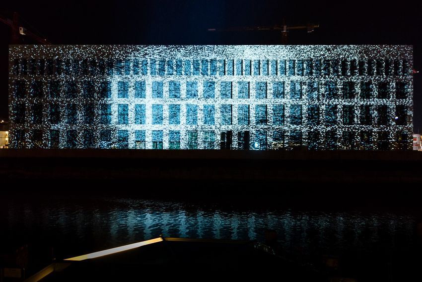
This thesis consists of material all of which I authored or co-authored: see Statement
of Contributions included in the thesis. This is a true copy of the thesis, including any
required final revisions, as accepted by my examiners.

I understand that my thesis may be made electronically available to the public.

                                           ii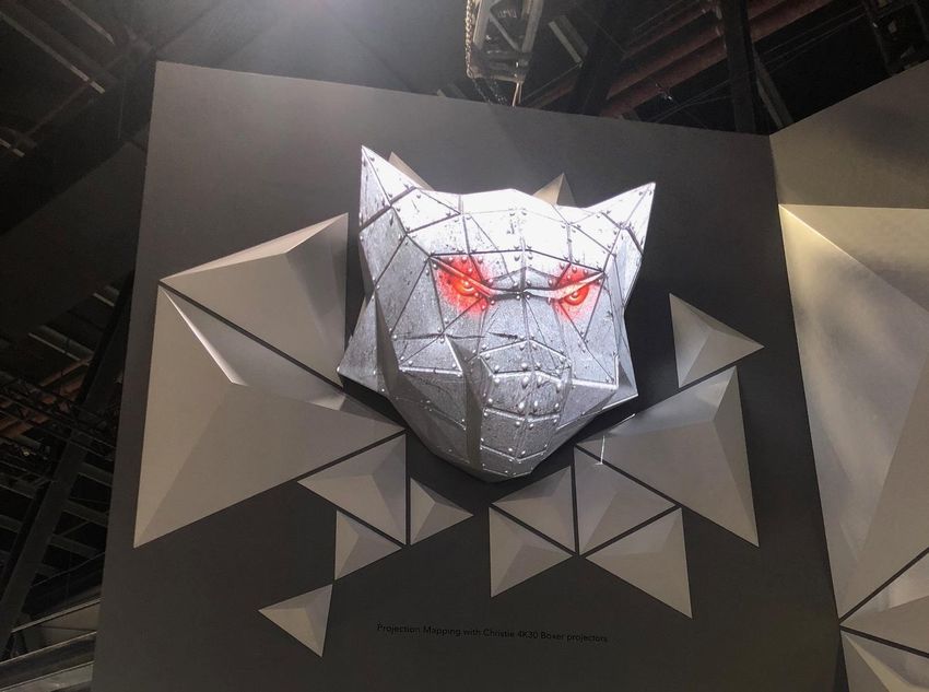
Statement of Contribution

The thesis is based on the following papers. I am the first author and have contributed
to the implementation, experimentation, and writing of all the papers. The content of
Chapter 4 has been taken from paper (1) and majority of the content presented in Chapter 5
has been documented in paper (2) & (3).

  1. V. Sankar, A. Gawish, and P. Fieguth. “Impact of Training Images on Radiometric
     Compensation.” Journal of Computational Vision and Imaging Systems. 3.1 (2017).

  2. V. Sankar, A. Gawish, P. Fieguth, and M. Lamm. “Understanding Blur and Model
     Learning in Projector Compensation.” Journal of Computational Vision and Imaging
     Systems. (2018).

  3. V. Sankar, A. Gawish, P. Fieguth, and M. Lamm. “ILRC: Inversely Learned Radio-
     metric Compensation.” IEEE Transactions on Visualization and Computer Graph-
     ics. submitted in August, 2018.

                                            iii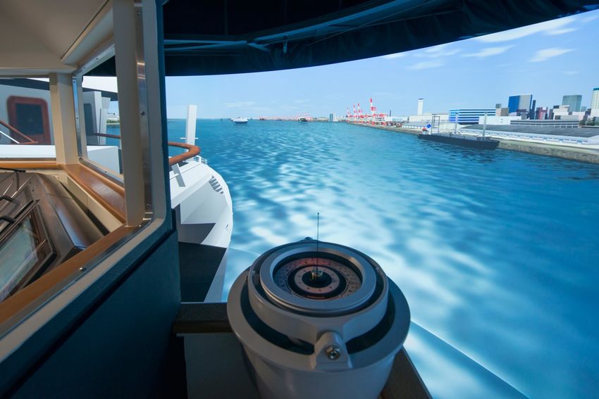
Abstract

    Projecting onto irregular textured surfaces found on buildings, automobiles and theatre
stages calls for the development of radiometric and geometric compensation algorithms that
require no user intervention and compensate for the patterning and colourization of the
background surface. This process needs a projector–camera setup where the feedback from
the camera is used to learn the background’s geometric and radiometric properties. In
this thesis, radiometric compensation, which is used to correct for the background texture
distortion, is discussed in detail. Existing compensation frameworks assume no inter–
pixel coupling and develop an independent compensation model for each projector pixel.
This assumption is valid on background with uniform texture variation but fails at sharp
contrast differences leading to visible edge artifacts in the compensated image.
    To overcome the edge artifacts, a novel radiometric compensation approach is presented
that directly learns the compensation model, rather than inverting a learned forward model.
That is, the proposed method uses spatially uniform camera images to learn the projector
images that successfully hide the background. The proposed approach can be used with
any existing radiometric compensation algorithm to improve its performance. Comparisons
with classical and state-of-the-art methods show the superiority of the proposed method
in terms of the perceived image quality and computational complexity.
    The modified target image from the radiometric compensation algorithm can exceed
the limited dynamic range of the projector resulting in saturation artifacts in the compen-
sated image. Since the achievable range of luminance on the background surface with the
given projector is limited, the projector compensation should also consider the contents
of the target image along with the background properties while calculating the projector
image. A novel spatially optimized luminance modification approach is proposed using
human visual system properties to reduce the saturation artifacts. Here, the tolerance of
the human visual system is exploited to make perceptually less sensitive modifications to
the target image that in turn reduces the luminance demands from the projector. The pro-
posed spatial modification approach can be combined with any radiometric compensation
models to improve its performance. The simulated results of the proposed luminance mod-
ification are evaluated to show the improvement in perceptual performance. The inverse
approach combined with the spatial luminance modification concludes the proposed pro-
jector compensation, which enables the optimum compensated projection on an arbitrary
background surface.

                                            iv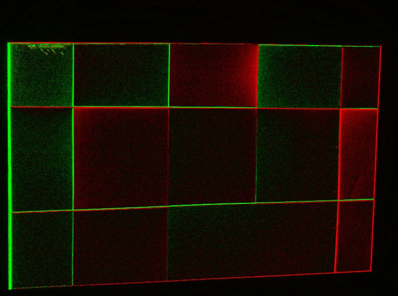
Acknowledgements

    First and foremost, I would like to thank my supervisors, Prof. Paul Fieguth and Prof.
David Clausi for their constant support, guidance, and motivation throughout my degree.
In addition, I wish to thank my co-author Dr. Ahmed Gawish for his inputs and suggestions
in writing papers and conducting research.
   I want to thank Christie Digital Systems for providing equipment, workspace, and
support for my research. I would also like to acknowledge the assistance of Mark Lamm
from Christie Digital Systems for his insights and suggestions.
    I would like to convey my gratitude to the Vision and Image Processing lab for creating
a healthy environment to conduct research. I am also grateful to the Ontario Centres of Ex-
cellence — Voucher for Innovation and Productivity II (OCE-VIPII), the Natural Sciences
and Engineering Research Council of Canada — Collaborative Research and Development
(NSERC-CRD) for sponsoring this research.
   My special thanks to Prof. Jeff Orchard and Prof. Bryan Tripp for taking their time to
review my thesis and provide valuable feedback.
   Finally, I would like to thank my parents, N. Sankar and S. Bhanumathi, and my sister,
S. Mohana Priya, for their continuous support and encouragement.

                                            v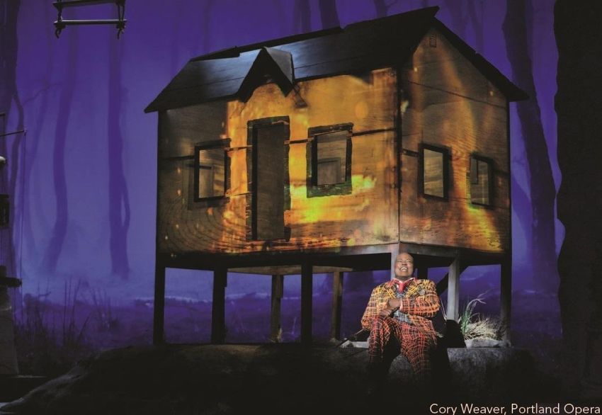
Dedication

This is dedicated to my parents.

                                       vi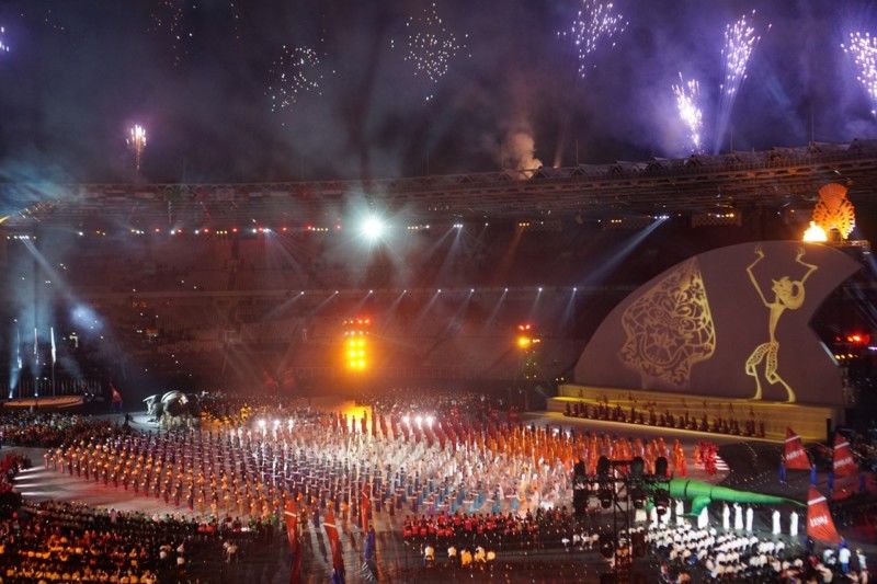
Table of Contents

List of Tables                                                                                 x

List of Figures                                                                                xi

1 Introduction                                                                                 1
   1.1   Motivation . . . . . . . . . . . . . . . . . . . . . . . . . . . . . . . . . . . .     1
   1.2   Problem Statement . . . . . . . . . . . . . . . . . . . . . . . . . . . . . . .        3
   1.3   Thesis Contribution and Organization        . . . . . . . . . . . . . . . . . . . .    4

2 Literature Review                                                                            5
   2.1   Introduction . . . . . . . . . . . . . . . . . . . . . . . . . . . . . . . . . . .     5
   2.2   Camera and Projector Response Function . . . . . . . . . . . . . . . . . .             6
   2.3   Geometric Calibration . . . . . . . . . . . . . . . . . . . . . . . . . . . . .        6
   2.4   Radiometric Compensation . . . . . . . . . . . . . . . . . . . . . . . . . . .         7
         2.4.1   Linear Models . . . . . . . . . . . . . . . . . . . . . . . . . . . . . .      8
         2.4.2   Non-Linear Models . . . . . . . . . . . . . . . . . . . . . . . . . . .       10
   2.5   Image Enhancements . . . . . . . . . . . . . . . . . . . . . . . . . . . . . .        10
         2.5.1   Multi–Projector Setup . . . . . . . . . . . . . . . . . . . . . . . . .       11
         2.5.2   Gamut Mapping . . . . . . . . . . . . . . . . . . . . . . . . . . . .         11
         2.5.3   Anchoring Theory . . . . . . . . . . . . . . . . . . . . . . . . . . . .      12
         2.5.4   Human Visual System . . . . . . . . . . . . . . . . . . . . . . . . .         12
   2.6   Summary . . . . . . . . . . . . . . . . . . . . . . . . . . . . . . . . . . . .       13

                                              vii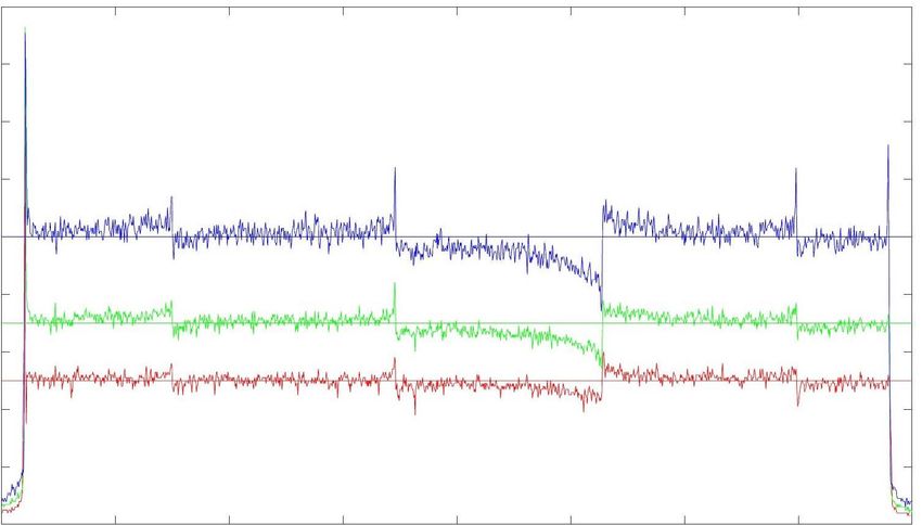
3 Projector–Camera Setup                                                                      14
  3.1   Camera Calibration . . . . . . . . . . . . . . . . . . . . . . . . . . . . . . .      14
  3.2   Projector Calibration . . . . . . . . . . . . . . . . . . . . . . . . . . . . . .     17
  3.3   Projector–Camera setup . . . . . . . . . . . . . . . . . . . . . . . . . . . .        18

4 Limitations of Radiometric Compensation                                                     19
  4.1   Brightness Leakage . . . . . . . . . . . . . . . . . . . . . . . . . . . . . . .      20
  4.2   Theoretical Analysis of Inter–Pixel Coupling . . . . . . . . . . . . . . . . .        23
  4.3   Experimental Observation . . . . . . . . . . . . . . . . . . . . . . . . . . .        24

5 Radiometric Artifacts                                                                       29
  5.1   Iterative Approach . . . . . . . . . . . . . . . . . . . . . . . . . . . . . . .      30
  5.2   Experimental Setup & Results . . . . . . . . . . . . . . . . . . . . . . . . .        32
        5.2.1   Implementation . . . . . . . . . . . . . . . . . . . . . . . . . . . . .      35
        5.2.2   Comparison Methods . . . . . . . . . . . . . . . . . . . . . . . . . .        35
        5.2.3   Evaluation Metrics . . . . . . . . . . . . . . . . . . . . . . . . . . .      36
        5.2.4   Results . . . . . . . . . . . . . . . . . . . . . . . . . . . . . . . . . .   36
        5.2.5   Edge Error Metric . . . . . . . . . . . . . . . . . . . . . . . . . . .       38
  5.3   Summary . . . . . . . . . . . . . . . . . . . . . . . . . . . . . . . . . . . .       39

6 Image Enhancement                                                                           43
  6.1   Introduction . . . . . . . . . . . . . . . . . . . . . . . . . . . . . . . . . . .    43
  6.2   Saturation Artifacts . . . . . . . . . . . . . . . . . . . . . . . . . . . . . . .    44
  6.3   Artifact Sensitivity . . . . . . . . . . . . . . . . . . . . . . . . . . . . . . .    45
        6.3.1   Saturated Regions . . . . . . . . . . . . . . . . . . . . . . . . . . .       47
        6.3.2   Pixel–Wise Correction . . . . . . . . . . . . . . . . . . . . . . . . .       47
        6.3.3   Spatial Correction    . . . . . . . . . . . . . . . . . . . . . . . . . . .   50
  6.4   Experiments & Results . . . . . . . . . . . . . . . . . . . . . . . . . . . . .       53
  6.5   Summary . . . . . . . . . . . . . . . . . . . . . . . . . . . . . . . . . . . .       55

                                              viii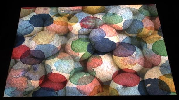
7 Conclusion                                                                                57
  7.1   Summary . . . . . . . . . . . . . . . . . . . . . . . . . . . . . . . . . . . .     57
  7.2   Future Work . . . . . . . . . . . . . . . . . . . . . . . . . . . . . . . . . . .   58

References                                                                                  60

                                             ix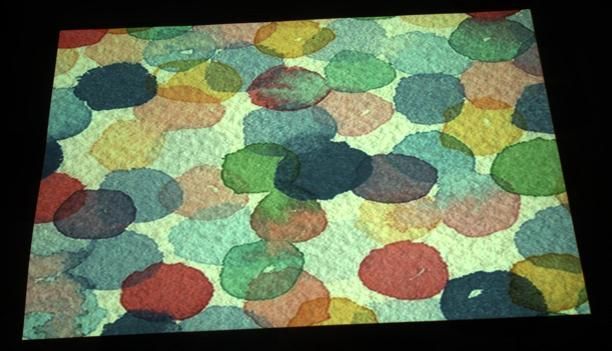
List of Tables

 5.1   RMSE, CIE2000 and SSIM scores for compensation on colored background           34
 5.2   Median edge score for Colored background . . . . . . . . . . . . . . . . . .   40
 5.3   Computational complexity comparison during calibration. . . . . . . . . . .    41

                                          x
List of Figures
1.1 Application of the projection technology by Christie Digital Systems . . . . 2
2.1 Gray scale pattern images . . . . . . . . . . . . . . . . . . . . . . . . . . . 7
3.1 Projector–Camera system for projector compensation. . . . . . . . . . . . . 15
3.2 Projector–Camera system used for experiments . . . . . . . . . . . . . . . 16
3.3 Camera image in projector coordinate system . . . . . . . . . . . . . . . . 17
4.1 Brightness leakage of projector–camera system . . . . . . . . . . . . . . . . 21
4.2 Results of Yoshida’s radiometric compensation model . . . . . . . . . . . . 22
4.3 Yoshida’s compensated camera image intensity distribution . . . . . . . . . 23
4.4 Conventional calibration set . . . . . . . . . . . . . . . . . . . . . . . . . . 24
4.5 Results of compensation by uniform and non-uniform calibration images . 25
4.6 Analysis of the compensated camera image’s artifact. . . . . . . . . . . . . 27
5.1 Conventional calibration set . . . . . . . . . . . . . . . . . . . . . . . . . . 31
5.2 Proposed calibration set . . . . . . . . . . . . . . . . . . . . . . . . . . . . 31
5.3 Background Images . . . . . . . . . . . . . . . . . . . . . . . . . . . . . . . 32
5.4 Target images used to evaluate the performance of the proposed model on
colored background . . . . . . . . . . . . . . . . . . . . . . . . . . . . . . . 33
5.5 Results of the proposed model on colored background . . . . . . . . . . . . 33
5.6 Target images used to evaluate the performance of the proposed model on
monochrome background . . . . . . . . . . . . . . . . . . . . . . . . . . . . 37
xi5.7 Results of the proposed model on monochrome background . . . . . . . . . 37
5.8 RMSE, CIE2000 error map for proposed and state of the art non–linear model 41
5.9 Median based metric to penalize edge like artifacts sensitive to human visual
system . . . . . . . . . . . . . . . . . . . . . . . . . . . . . . . . . . . . . . 42
6.1 Flowchart of the image enhancement techniques . . . . . . . . . . . . . . . 44
6.2 Results of simulated compensation by Yoshida’s linear model . . . . . . . . 46
6.3 Upper and Lower saturated regions . . . . . . . . . . . . . . . . . . . . . . 46
6.4 Median filtered saturation map . . . . . . . . . . . . . . . . . . . . . . . . 48
6.5 Proposed pixel–wise luminance correction. . . . . . . . . . . . . . . . . . . 50
6.6 Comparison of spatial modification for different slope values . . . . . . . . 52
6.7 Results of Linear and Gaussian kernel based spatial modification . . . . . . 54
6.8 Target Images used to evaluate the performance of the proposed spatial
modification approach. . . . . . . . . . . . . . . . . . . . . . . . . . . . . . 56
6.9 Comparison of the simulated result by proposed spatial correction with
global, pixel–wise modified target image. . . . . . . . . . . . . . . . . . . . 56
xiiChapter 1
Introduction
1.1 Motivation
Projector technology [37, 58, 30, 28] has been revolutionized in the last decade and it
continues to increase the achievable resolution and contrast ratio of modern projectors. The
power consumption and size of the projectors is also reducing dramatically [17] to make
the projectors more portable. The rapidly increasing availability of high-end portable
projectors has led to the increased use of three-dimensional objects, such as buildings,
automobiles, and artistic structures, as projection surfaces for high-definition displays.
Currently, projectors are used in every automobile show to highlight various features of
a car. Projectors are also used during ceremonies and in theaters to dynamically change
the perception of the scene on the stage. Niagara falls is regularly illuminated by the
high–end laser projectors to attract more visitors during holidays. Disney theme parks are
well known for using large scale projections as a part of their entertainment. On a smaller
scale, projection technology can be used with 3D objects to create non-intrusive virtual
reality experiences. Museums and art exhibitions have used this technology to restore the
appearance of degraded artistic structures. Also, the emergence of the pocket sized pico
projectors [17] has led to widespread use of projectors in households. Pico projectors are
an affordable option to achieve High–Definition theatre experience on the go. More and
more people are opting for the affordable high-end projectors, instead of a traditional LCD
screen, for media consumption.
The ubiquitous use of projectors in households is only limited by the unavailability
of projection screens. To obtain the stated resolution and contrast, a high quality pro-
jection screen is needed for the entire projection area. The currently available projection
1(a) (b) (c)
(d) (e) (f)
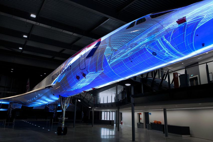
Figure 1.1: Application of the projection technology by Christie Digital Systems in (a) 2018
Asian paralympic games, (b) illumination of Berlin palace, (c) theatre illumination, (d)
360-degree ship bridge simulator, (e) 3D projections and (f) to restore a decommissioned
plane1 . The projector technology is successful in compensating for the 3D nature of the
underlying object. However, the texture of the surface is still causing visible artifacts in
the projection.
screens are substantial in size and are commonly expensive for household usage. Hence
there is a need for modern projectors to shift from using a traditional projection screen
to a nearby surface for projection. Using an arbitrary surface requires manual calibration
to correct for image distortions. For projection on non-planar and 3D objects, projec-
tors use geometric calibration to model the shape of the object and correct for structural
distortions. However, modern projectors fail to compensate for the background texture.
Existing approaches use high luminance projectors to mask the background texture, which
is expensive. Otherwise, manual calibration is needed to neutralize the distortions, which
consumes an enormous amount of time. Image processing techniques[47, 27] can be used
to automatically understand the surface characteristics and use it to modify the target
image such that un-distorted projections can be obtained on the surface. In this thesis,
we explore different image processing techniques which can be used to develop automatic
real–time projector compensation without human interference.
21.2 Problem Statement
Projector compensation is the process of achieving un–distorted image or video on a non-
planar and textured background. It involves correcting for the geometric and radiometric
distortions of the background. A projector–camera setup is used to understand the required
surface properties [47]. A geometric model is developed from the learned properties that
define the structure of the surface from the view point of the camera [53, 6, 31]. Geometric
calibration results in an un–distorted image on the background surface which is degraded by
the underlying texture of the surface. Radiometric compensation, which can correct for the
texture degradation, is developed by projecting and capturing a series of colored images and
using them to understand the surface’s texture properties [47, 27, 64]. The compensation
model, developed from the learned properties, modifies the intensities of the image with
respect to the background such that the modified image combines with the background
surface to present the desired image without any degradation. In case of a radiometrically
extreme background surface or a limited dynamic range projector, image enhancement
techniques [60, 26, 30] can be used as a part of projector compensation to reduce the
brightness demands on the projector and obtain an optimum projector performance.
Geometric calibration is a well studied problem and current state of the art models can
achieve sub-pixel accuracy from the camera viewpoint [63, 39]. Radiometric compensation
is developed on top of the given geometric calibration model. The current radiometric
framework uses a pixel–based approach, where a compensation function is developed for
each projector pixel. Each compensation model is developed independently and the frame-
work assumes no inference between adjacent pixels [47, 25]. This assumption works for
background surface with smooth texture variations but fails at the background edges with
sharp contrast difference [47].
The main aim of projector compensation is to reduce the perceptual difference between
the desired target image and the compensated image on the background surface. Since the
corrections are made with respect to the camera, the objective is to reduce the error between
the target image and the compensated camera image. Two types of errors are encountered
during compensation: the radiometric error, due to the incorrect learning/modelling of
the background properties, and the saturation error, because of the physical limitations of
the projector [28]. The projector compensation framework should be designed to minimize
both radiometric and saturation error. The objective of this thesis is to provide a robust
projector compensation framework, which can be used with any projector and camera
1
Images are taken from Christie Digital Systems linkedin page:
https://www.linkedin.com/company/christie-digital-systems/
3to provide the perceptually optimum projection of the desired image on any background
surface.
1.3 Thesis Contribution and Organization
The next chapter reviews the current literature on different components of the projector
compensation framework. State of the art models for the camera, projector and geo-
metric calibration are provided. Different radiometric compensation models are discussed
by categorizing them into the linear and non-linear model. Various image enhancement
techniques which are proposed for improving the perceptual performance of the projector
compensation are also discussed.
The projector–camera setup required for the compensation framework is discussed in
Chapter 3. The necessary camera and projector calibration to be performed as a part of
the experimental setup is elaborated. Since the camera forms the eye of the setup, the
influence of camera parameters on the performance of the compensation model is examined
in detail.
Chapter 4 discusses the assumptions of the existing radiometric compensation algo-
rithms. Notably, the assumption of no interference between pixels is examined in detail.
Experimental verification was provided by developing the same radiometric compensation
model with different calibration sets to prove that the assumption will lead to artifacts at
the background texture’s edge.
Inspired from the results of Chapter 4, a novel inverse framework is proposed in Chap-
ter 5, which can be used with any radiometric compensation algorithm to improve its per-
formance. The proposed framework inherently learns the inter–pixel dependencies without
an increase in computational complexity. The results of the inverse model are compared
with the linear and state of the art non-linear models to justify the improvement in per-
formance.
To reduce the brightness demands of the projector, a novel luminance modification ap-
proach is proposed in Chapter 6. Here, the modification is localized and spatially optimized
for the human visual system. This approach can be used with the proposed or existing
radiometric models to reduce artifacts due to device limitations. The combination of the
inverse model with the spatially optimized luminance modification concludes the proposed
projector compensation framework.
4Chapter 2
Literature Review
2.1 Introduction
Radiometric compensation is the process of manipulating the incoming image to a projector
such that the projected image modulates with the background to provide the desired
appearance for an observer. This process utilizes a projector–camera system such that
the projector projects an image onto the background surface, and the camera provides
feedback in order to learn the geometric and radiometric properties of the surface. For a
given target image, the compensated projector image is obtained by modifying the target
image with respect to the learned properties. Projecting the compensated image gives the
appearance of a non-distorted target image on the surface.
Imaging systems, such as camera and projector, have an inherent non-linear response
while converting the digital intensity values to/from the scene irradiance. These responses
are modelled as the radiometric response function. This chapter starts by reviewing the
literature on the camera response function required for radiometric compensation. The ge-
ometric calibration needed to map the camera and projector image pixels are discussed in
Section 2.3. Existing radiometric compensation along with the state of the art algorithms
are discussed in detail. In conjunction with radiometric compensation, image enhance-
ment techniques are proposed in the literature to improve the perceptual quality of the
compensated image. In general, the proposed techniques are used to reduce the saturation
artifacts encountered due to the limited dynamic range of the projector.
52.2 Camera and Projector Response Function
In most imaging systems [22], there is a non-linear relationship between the scene irradiance
reading and the digital intensity values. The non-linearity can be due to the inherent
gamma mapping in the device, analog/digital conversion, or introduced intentionally by the
manufacturer to enhance the visual quality. Computer vision applications model the non-
linearity as the response function of the device and uses it to establish linear relationship
between the intensity values and scene irradiance. Extensive research has been done in
the field of camera response functions [22, 24, 21, 23, 38, 21, 4, 33]. The most common
approach uses a set of images captured with varying exposure values to calculate the
camera response function [13, 41, 44]. Lin and Matsushita et al. [42] proposed to use
noise distribution in the image to find the required function. Lee et al. [35] proposed a
rank minimization framework to solve for the response function. Modern projectors have
the manual setting to change the inherent non-linearity. But for traditional projectors,
Grossberg et al. [25] proposed a framework to calculate the projector response function
along with the radiometric compensation model assuming camera response function is
known.
2.3 Geometric Calibration
After camera calibration with the radiometric response function, the geometric calibration
between the projector and camera should be obtained. The pixel correspondence from the
mapping is necessary to correlate the camera pixels to its corresponding projector pixels.
The geometric calibration is calculated for a fixed projector–camera setup. Structured
light patterns [53, 6, 31] are used to obtain geometric calibration for planar or non-planar
textured backgrounds. Salvi et al. [53] provides a comprehensive review of the existing geo-
metric calibration algorithms. Gray code structured light projection proposed by Inokuchi
et al. [31] uses a sequence of m binary coded image pattern as shown in Fig 2.1 with
hamming distance of one between images to encode 2m pixels. Each pixel in the projector
image is marked by the unique binary code and the captured camera image’s pixels are
decoded to find its corresponding projector pixel. Sansoni et al. [55] and Wiora et al. [63]
proposed to use a combination of gray code and phase shift coding to achieve sub-pixel
accuracy. The acquired geometric calibration between projector and camera is also used
to compensate for the geometric distortion caused by the background surface.
In order to support dynamic projector–camera setting, Park et al. [48] embedded the
structured light pattern with incoming projector images and simultaneously detected and
6(a) Projector images
(b) Camera images
Figure 2.1: Examples of gray scale structured light pattern. Every pixel in the projector
image is encoded using (a) the binary coded image sequence and (b) the camera image
pixel values are decoded to find the corresponding projector pixel.
corrected for any change in projector–camera setup in real time. Recently, Bokaris et al. [8]
proposed a robust calibration model by analyzing the characterization of DLP projectors,
and proposed an algorithm which can achieve complete re-calibration with just one frame
delay.
2.4 Radiometric Compensation
Radiometric compensation is required to correct for the projection image’s texture distor-
tion due to the background surface. To understand the surface’s texture characteristics,
a calibration set is formed by projecting a series of colored images and capturing their
responses. The radiometric functions fr developed from the calibration set, model the
transformation of the projector image intensity P (x1 , y1 ) by the projection surface to pro-
duce the captured camera image intensity C(x2 , y2 ):
C(x2 , y2 ) = fr (P (x1 , y1 )) (2.1)
Where projector image’s pixel location at (x1 , y1 ) corresponds to camera image’s pixel
location at (x2 , y2 ). The function is developed for each projector–camera pixel pair, as
7the background texture and colour can vary, essentially arbitrarily, from pixel to pixel.
The radiometric function is inverted to form the compensation function fr−1 , which can be
applied to the target image intensity T (x1 , y1 ) to yield the compensated projector image
intensity Pc (x1 , y1 ):
Pc (x1 , y1 ) = fr−1 (T (x1 , y1 )) (2.2)
Cc = S(Pc ) (2.3)
where S represents the transformation by the background surface. Cc is the camera cap-
tured compensated image, ideally equivalent to the target image T . Since the radiometric
function is developed for each projector pixel, it is necessary for the model to be simple and
efficient. Different Models are used to define the different radiometric function depending
on the scenario at hand. Broadly, radiometric functions can be categorized into either
linear or non-linear models. The following subsection discuss each category in detail.
2.4.1 Linear Models
For a projector–camera system, Nayar et al. [47] proposed to model the input irradiance
of the camera CL for channel L in terms of the brightness output of the projector PK for
channel K as XZ
CL = wK (λ)S(λ)qL (λ)PK dλ (2.4)
K
Here, wK is the spectral response of the projector for channel K, S is the spectral reflectance
of the surface in the viewing direction of the camera, and qL is the quantum efficiency of
the camera for channel L. The Projector IP and Camera IC pixel values are related to the
irradiance values as follows,
PK = rP (IP ) (2.5)
IC = rC (CL ) (2.6)
where rP and rC represent the projector and camera response function. For a three color
channel projector–camera system, (2.4) can be represented as
C = V P, (2.7)
where
cR vRR vRG vRB pR
C = cG , V = vGR vGG vGB , P = pG
(2.8)
cB vBR vBG vBB pB
8Z
vKL = wK (λ)s(λ)qL (λ)dλ (2.9)
In principle the camera’s and projector’s spectral responses can overlap with each other in
arbitrary ways [47], so it is necessary for the radiometric model to be able to capture all
inter-channel dependencies. The model in (2.7) separates the non-linear projector/camera
response function from the radiometric function and uses a linear system of equations to
model the transformation of the projector brightness output. The color mixing matrix V
captures the coupling of the camera and projector color channels and their interaction with
the spectral reflectance of the background [47]. As with f (), the color mixing matrix V
needs to be modelled separately for every projector pixel.
Yoshida et al. [64] improved Nayar’s model in (2.7) by adding a constant term to
consider the effects of environmental light and projector offset as
C = V P + K, (2.10)
where
vRR vRG vRB pR kR
V = vGR vGG vGB , P = pG , K = kG
(2.11)
vBR vBG vBB pB kB
Bimber et al. [7] proposed a channel independent model, where the radiometric function
is modeled as a diagonal matrix, thus the model does not consider the spectral response
overlap between the projector and camera. Grossberg et al. [25] proposed to use a minimal
set of six images to calculate the color mixing matrix V and projector response function.
Lee et al. [36] increased the speed of the radiometric compensation by eliminating the
spectral overlap using color filters and modelling the color mixing matrix as a diagonal
matrix. Chen et al. [10] studied the color mixing property of the projector–camera system
and presented a method to separate the spectral overlap matrix from the color mixing
matrix, where a single matrix was then calculated for the entire system to describe the
spectral overlap between the projector and camera. Futji et al. [18] extended the linear
model for dynamic environments by using a co-axial projector–camera system where the
geometric correspondence between the projector and the camera is independent of envi-
ronmental changes. Here, the color mixing matrix V was separated into a diagonal matrix
A, which captures the spectral reflectance of the surface, and dense Vf , which represents
the overlap between the projector and camera spectral responses:
C = AVf P 0 (2.12)
A is calculated for each projector pixel whereas, a single Vf matrix is used for all projec-
tor pixels. Mihara et al. [43] proposed a compensation model, which uses a high spatial
9resolution camera to capture the background spectral reflectance variation inside a single
projector pixel, such that Yoshida’s linear model (2.10) is developed for each of the multiple
camera pixels within a projector pixel.
The previously mentioned models assumes a Lambertian surface for the projection
background. Park et al. [49] used multiple projectors and camera to use a non–Lambertian
surfaces for projection. Here, the projectors are arranged such that at least one diffuse
projector is available for each point at the projection surface which does not produce
specular reflection for a given camera viewpoint.
2.4.2 Non-Linear Models
Chiu et al. [11] used the projector–camera system and a non-linear radiometric compen-
sation model to remove the textured content on presenter’s face during presentation. A
non-linear radiometric model, based on (2.7), was presented along with an adaptation
scheme for dynamic ambient light. The per-pixel linear model was extented to a cubic
version as follows,
pcubic
P 0 = pquadratic (2.13)
plinear
Grundhofer et al. [28, 27] proposed a non-linear compensation model, which does not
require pre-calibration of the camera or projector response function. The algorithm uses
a sparse sampling of the projector gamut and thin plate spline interpolation to generate
the mapping from the projector’s input image to output image of the camera in RGB
space. The target image is automatically scaled to maximize the achievable luminance and
contrast [28].
Both linear and non-linear models assume each camera pixel intensity depends on only
one projector pixel intensity and environmental light. But in practical scenarios, there is
inter–pixel coupling between projector pixels resulting in many-to-many relationships be-
tween the projector and camera. The limitations of the discussed radiometric compensation
models are discussed in Chapter 4.
2.5 Image Enhancements
The compensated projector image Pc calculated from the linear or non-linear model does
not consider the physical limitations of the projector or camera. In practical scenarios, Pc
10intensity values can go beyond the dynamic range of the projector. The projector clips the
image values at its limits and projects a saturated image. Since the required brightness is
not projected on the given background, the compensated camera image Cc deviates from
the target image leading to artifacts at the saturated regions. The saturation artifacts are
not due to the incorrect learning of the background surface, and are caused by the limited
dynamic range of the projector.
2.5.1 Multi–Projector Setup
Different approaches are proposed in the literature to solve for saturation artifacts. Multi-
ple projectors can be used to solve for the limited dynamic range of a single projector, by
using more then one projector to attain the required brightness level that hides the back-
ground texture. Bimber et al. [7] proposed to use multiple projectors, where the required
brightness is distributed evenly among all the overlapping projectors for a given point on
the projection surface. Miyagawa et al. [45] used state equations, which are controlled
using camera feedback, to distribute brightness among multiple projectors. Tsukamoto
et al. [59] came up with multiple projector brightness distribution framework using two
Degree of Freedom (DOF) control structure. Here, the communication bandwidth is op-
timized by using a centralized feed–forward mechanism. Theoretical and experimental
verification was provided to demonstrate the successful performance in still and moving
images.
2.5.2 Gamut Mapping
Multiple projectors can effectively solve the limited brightness capability of a single projec-
tor, but it also increases the overall complexity and cost of the required setup. Saturation
artifacts can be reduced with a single projector by modifying the contrast of the incoming
images to fit inside the projector gamut. Ashdown et al. [5] presented a five stage frame-
work where the target image is first converted to a perceptual uniform CIELUV color
space. Chrominance and luminance fitting was carried out in the CIELUV color space, as
linear change in this color space will lead to linear changes in perceptual sensitivity. The
fitted target image is converted to RGB color space and combined with the radiometric
compensation algorithms for projection. Park et al. [50] proposed to use a local adaptive
mapping depending on the projection surface and target image intensity for each pixel.
The adaptive mapping function is constrained to have smooth variation across pixels to
avoid abrupt color changes. Huang et al. [29] decoupled the surface reflectance properties
11from the color mixing matrix and then proposed luminance reallocation to solve for the
clipping errors.
2.5.3 Anchoring Theory
Anchoring theory of lightness perception [19] is also used to solve for saturation artifacts.
Luminance is a physical quantity which can be measured. Lightness, on the other hand,
is a subjective brightness perceived by the human visual system. Lightness of a scene is
determined by the brightest point of the scene or “anchoring point”. The human visual
system first spots the anchoring point and identifies it as white and then perceives the
lightness of scene with respect to the anchoring point. Wang et al. [61] proposed to use the
anchoring theory for brightness scaling and hue adjustments. The algorithm identifies and
scales the value of the anchor point using the CIECAM02 [46] color appearance model.
Huang et al. [30] extented the model and put forth a radiometric compensation framework
using anchoring theory to reduce clipping errors and to improve the overall quality of
the compensated image. Subjective tests were conducted to verify the superiority of the
proposed framework.
2.5.4 Human Visual System
Ramasubramanian et al. [52] used human visual system properties derived from exper-
imental data to calculate the threshold map of an image given its viewing conditions.
The threshold map incorporates the luminance masking, contrast sensitivity and contrast
masking properties to calculate the maximum possible luminance deviation for a particular
pixel until the human visual system notices the difference. This threshold is calculated for
each pixel separately and combines together to form the threshold map. The properties of
the threshold map was used by Wang et al. [60] to calculate the global scaling factor which
optimizes the trade off between overall brightness and saturation artifact error. Grund-
hofer et al. [26] used the threshold map to propose global and local changes to the target
image to reduce the saturation artifact. The global changes depend on the saturation error
and average luminance of the image. The local changes are calculated by the Gaussian
smoothed saturation error and the changes are limited by the values from the threshold
map. Temporal adaption for the global change is also provided as the part of the paper.
122.6 Summary
In this chapter, different components of the projector–camera system were discussed. Most
commonly used camera response function and geometric calibration algorithms were pre-
sented along with recent advances. Linear and non-linear radiometric compensation algo-
rithms were discussed in detail. Image enhancements methods used in combination with
radiometric compensation models were categorized and state of the art solution in each
category was explained. Next, Chapter 3 explains the projector–camera setup in detail.
Chapter 4 discusses the common assumptions and limitations in the existing radiometric
compensation models.
13Chapter 3
Projector–Camera Setup
In the previous chapter, we discussed the state of the art radiometric compensation and im-
age enhancement techniques. The compensation models require a projector–camera setup
as shown in Fig 3.1. The camera provides continuous feedback of the projection, which
can be used to learn the geometric and surface reflectance properties of the background.
The learned properties are used to make corrections to the incoming image. Here, all the
corrections are made with respect to the position and reading of the camera. For different
position and viewing angles of the observer, the background reflectance properties of the
projection surface changes. Hence, the developed geometric model is valid only near the
camera viewpoint. As the observer moves away from the camera viewpoint, the compen-
sated image starts to deviate from the desired image. Similarly, the radiometric corrections
are made with respect to the intensity values captured by the camera. In this chapter,
we discuss the parameters of the camera and their influence on the performance of the
compensation. The details of the projector–camera setup used for the implementation of
the geometric and radiometric models are also explained.
3.1 Camera Calibration
A 5M-pixel Gigabit Ethernet machine vision camera is used as a part of the projector–
camera setup. The camera should be calibrated to have a monotonic response to the
projector intensity values considering most of the existing radiometric models [47, 64,
25] assume a linear relationship between the projector and camera. Since cameras are
developed to capture maximum details of the scene, different image processing techniques
are embedded as part of the image capturing process [44]. One of the main purpose of
14Figure 3.1: Projector–camera system for radiometric compensation. The camera provides
a continuous feedback to understand the surface reflectance properties of the projector
screen.
the embedded techniques is to automatically choose the white balance and exposure value
of the camera. White balance defines the sensitivity of the RGB channels to different
environmental conditions, which in turn affect the chrominance reading of the camera
[3]. Different white balance settings lead to different chrominance readings of the static
scene. Similarly, the exposure of the camera affects the luminance reading of the scene
[34]. Automatic adjustment of white balance and exposure by the camera will lead to
inconsistent readings. Most modern cameras come with “automatic” adjustment as the
default setting for the white balance and exposure. In order to achieve monotonic response
for projector values, we need to have constant white balance and exposure value. In Point
Grey cameras, this was accomplished by manually changing the setting to have constant
exposure and white balance value in the software provided.
Having constant white balance and exposure value ensures a monotonic response for
the projector intensity values. In order to achieve a linear response, the camera’s gain and
gamma parameters values should be adjusted. Human perception of brightness approx-
imately follows a power function, where the relative difference between the darker level
of luminance is more sensitive than brighter levels [51]. The camera uses the following
gamma correction to take advantage of the brightness perception property to optimize the
bits usage while encoding an image:
Vout = Vinγ (3.1)
15Figure 3.2: Projector–Camera system used for experiments
where V is the camera intensity value. The camera response functions [42, 35, 25] explored
in Section 2.2 tries to model this gamma correction (3.1) of the camera. For the camera
used in the experiments, we have manually set γ to 1 in order to avoid the non-linear
transformation. Similarly, the gain of the camera [2] was set to 0 to avoid amplification.
By manually adjusting the camera parameters, we avoided the need to calibrate the camera
with the camera response function.
The linear response of the camera enables us to directly use the linear radiometric mod-
els discussed in Section 2.4.1. Since the compensation model uses the camera reading for
correction, the exposure value of the camera plays a significant role in model performance.
Different exposure values lead to different luminance readings of the same static scene [34].
Due to the limited dynamic range of the camera, an arbitrary exposure value can lead to
saturation of camera reading and incorrect learning of the background properties resulting
in artifacts in the compensated image. The aim of the camera is to capture the modulation
of the projector intensity with the background surface. Hence, the camera’s exposure value
should be calibrated to capture the entire range of the achievable luminance on the back-
ground surface. In our experiments, the shutter speed was varied between 50ms - 100ms
to control the exposure for different backgrounds.
The exposure values also act as the brightness parameter of the compensation image.
16(a) Camera image (b) Transformed camera image
Figure 3.3: The transformation of the (a) camera image into (b) the projector coordinate
system
The compensation model calculates the projector image value such that the modulation
with the background results in the desired intensity value on the compensated camera
image. A relatively higher exposure value will require low luminance demand from the
projector to achieve the desired intensity in the camera image. As we reduce the exposure
value of the camera and develop a new compensation model, the modified projector image
brightness is increased to attain the same desired intensity in the camera image. Hence
the brightness of the compensated image is inversely proportional to the exposure value
of the camera. This property can also be used to avoid saturation of the projector image
during radiometric compensation. The saturation of the projector is further discussed in
Chapter 6.
3.2 Projector Calibration
The Christie Digital single chip 1920 × 1200 DLP projector was used in our projector–
camera setup. The projector was connected to the computing device and used as a second
monitor to project the image. The gamma modification by the operating system for display
monitors was turned off to obtain a linear relationship between the projector and camera [1].
Similar to the camera, the non–linear transformation of the projector’s gamma correction,
was manually turned off to avoid the need for the projector response function.
173.3 Projector–Camera setup
The projector–camera setup of our experiment is shown in Fig 3.2. The camera is placed as
close as possible to the projector to reduce the geometric distortions on the camera image.
The entire setup was covered to ensure a minimum influence of ambient light. An exam-
ple of a camera image is shown in Fig 3.3. To extract meaningful background property
from the camera image, we require the camera–to–projector pixel location mapping. The
pixel correspondence was acquired from the geometric calibration process. The gray scale
structured light pattern [31] was used to obtain the geometric calibration as described in
Section 2.3. The calibration will help in transforming the camera image to the projector
coordinate system as shown in Fig 3.3. Having both the projector and camera image in
the same coordinate system helped us to directly compare the images and extract back-
ground properties. This transformation was also used to calculate the error between the
compensated camera image and the target image. The existing radiometric compensa-
tion frameworks [47, 27, 22] use pixel–level models developed for a static projector–camera
setup. Any change in the projector–camera setup will lead to incorrect pixel correspon-
dence and an ineffective compensation model. So the setup should remain static between
model development and compensation. The same projector–camera setup is used for all of
the experiments described in the following chapters.
18Chapter 4
Limitations of Radiometric
Compensation
We wish to examine the basic assumptions underlying the existing radiometric models and
their implications on the performance of the associated radiometric compensation algo-
rithms. The following assumptions are made in both the linear and non-linear radiometric
models:
• The camera is capable of capturing the entire range of the projector gamut without
saturation,
• Each camera pixel intensity is modelled as a function of only one projector pixel
intensity,
• Environmental light is constant during model development and validation.
The camera plays a significant role in radiometric compensation as it forms the eye of
the projector–camera system, and corrections to the projector image are made with respect
to the values of the camera image. The visual quality of the radiometric compensation
strongly depends on the ability of the camera to accurately capture the intensity and
contrast of the background surface. Due to constraints on the portability and cost of the
projector–camera system, off-the-shelf cameras with limited dynamic range are frequently
used in practical scenarios, and as a result the camera could become saturated and might
not be able to capture the entire range of the projector gamut. This saturation in the
calibration images would lead to artifacts in the compensated image.
19The radiometric function is developed for a static projector, camera, background and
environment. Recent advances have led to use of dynamic projection using a coaxial pro-
jector and camera setup and real time geometric calibrations [18]. But existing algorithms
still assume constant environmental light during radiometric function development and
evaluation. Outdoor projection or indoor projection with changing environmental bright-
ness can cause artifacts in the compensated camera image depending on the degree of
brightness variation.
In the projector–camera system, the luminance of one projector pixel can influence the
irradiance reading for multiple camera pixels, known as inter–pixel coupling [40], caused
by one or more of
• Projector optics,
• Projection surface, or
• Camera optics.
That is, a single projector pixel may affect a neighbourhood of camera pixels, and similarly
a camera pixel intensity may be a function of a neighbourhood of projector pixels. The
inter–pixel coupling makes the projector–camera system a many-to-many relation, over
some window size, where the extent of the window is determined by the nature or extent
of the inter–pixel coupling. Under this scenario, the forward approach fails, as the inverse
of the projector to camera transformation is not the same as the camera to projector
transformation. Hence, there is a need to find a more suitable approach to successfully
produce the target image on the background surface.
In this chapter, we look into the inter–pixel coupling in detail. The following section
discusses the brightness leakage which can be observed in the projector–camera setup due
to the inter–pixel coupling. The theoretical explanation is given for inter–pixel coupling by
stating that the projector point spread/blur function can distort the projector images. Ex-
perimental verification is provided by developing the widely used Yoshida’s [64] radiometric
compensation model in Eqn. (2.10) using different sets of projector images and evaluating
its performance under textured and plain background surface.
4.1 Brightness Leakage
For the background shown in Fig. 4.1a, let us consider the case in which only part of the
background screen is illuminated, as shown in Fig. 4.1b, which gives rise to the camera
20(a) Background (b) Projected image (c) Histogram equalized cam-
era image
Figure 4.1: Brightness leakage of the projector–camera system can be seen by (b) illumi-
nating a part of the projector screen and by (c) examining the histogram equalized camera
image of the projector screen. The illuminated regions affect the intensity reading of the
surrounding non-illuminated regions.
image of Fig. 4.1c, which has been histogram equalized [20] to bring out details. Although
only a square region was formally illuminated, the luminance of the illuminated region
is very obviously leaked to adjacent non-illuminated regions, including pixels quite some
distance away. As a result, the captured values in the non-illuminated regions are not an
appropriate function of the corresponding projector intensity since the radiometric model,
which does not consider inter–pixel coupling, associates these values as a contribution from
the background texture. The brightness leakage which is prominent at the projector image
edges or the background’s texture edges causes incorrect learning of the radiometric model
and leads to visible edges in the compensated camera images.
The results of Yoshida’s [64] linear model are shown in Fig. 4.2, from which it can
be observed that the linear model is able to compensate satisfactorily in uniform regions,
but the edges of the background remain visible in the compensated camera image. The
pixel intensities in a horizontal cross-section of the compensated camera image are plotted
in Fig. 4.3, showing that the compensated camera image intensity is deviating from the
target intensity in the vicinity of edges in the projected background. Similar effects can
be observed for all of the edges in the compensated camera image. The difference between
the target image and compensated camera image is shown in Fig. 4.2d. Red indicates the
positive values and green indicates negative values. We can observe significant deviation
at all the background edges and the quantity of deviation is proportional to the contrast
of the edge.
21(a) Projector screen (b) Target image
(c) Resulting compensated camera (d) Difference image (b) - (c)
image
Figure 4.2: Result of Yoshida’s extended linear model. Edges of the background are clearly
visible in the compensated result (c). The difference between the target and compensated
image is plotted in (d), where red indicates positive values suggesting lower luminance in
compensated image and green indicates negative values. The linear model works properly
in the uniform region but fails near the regions of contrast difference. The arrow in the
compensated camera image (upper right corner of (c)) identifies the row corresponding to
the plot in Fig. 4.3.
22180
160
140
Pixel Intensity Value
120
100
80
60
40
20
0
0 200 400 600 800 1000 1200 1400 1600
horizontal axis coordinate
Figure 4.3: Distribution of camera image intensities along a horizontal row as indicated by
the small arrow in Fig. 4.2c. The straight lines show the target values for each channel.
Clearly visible are the sharp deviations from target near regions of contrast difference in
the background.
4.2 Theoretical Analysis of Inter–Pixel Coupling
A major venue for inter–pixel coupling is at the projector. The point spread function of
the projector can blur the input image creating spatial dependencies. Since the blur of
the projector depends on the contents of the input image, different projector images in
the calibration set can lead to different performance by the compensation model. For a
spatially uniform projector image Pu , as shown in Fig. 4.4, the projector’s blur function
will not alter the intensities of the image:
B ∗ Pu = Pu (4.1)
As Pu does not contain any contrast, it will not be affected by the blur B. If the cali-
bration set is developed with similar projector–camera images, the radiometric function fˆ
calculated from this set will not be aware of the blur function of the projector:
fˆ = arg min kf (Pu ) − S(B ∗ Pu )k
f
(4.2)
= arg min kf (Pu ) − S(Pu )k
f
23(a) Projector image (b) Camera image
Figure 4.4: Conventional calibration set with spatially uniform projector image and camera
image of the projection.
where S represents the distortions by the background surface. The compensated projector
image Pc for a given target image T is calculated as follows,
Pc = fˆ−1 (T ) (4.3)
The calculated Pc , unlike the uniform projector images in calibration set Pu , will not be
spatially uniform in intensity. As the radiometric compensation model did not consider
the effect of B, distortion of the non-uniform Pc by the blur function B will necessarily
lead to artifacts in the compensated camera image:
B ∗ Pc 6= Pc (4.4)
S(B ∗ Pc ) 6= S(Pc ) = T (4.5)
Using spatially uniform projector images in the calibration set can cause artifacts in the
compensated camera image. Similarly, different kinds of projector images can lead to
various artifacts. So to understand the relationship between the projector image pattern
and the artifacts in the compensated image, we analyzed the error maps of the radiometric
compensation model developed with different sets of projector images.
4.3 Experimental Observation
Two calibration sets were constructed to examine the influence of inter–pixel coupling. The
first set contains textured projector images using natural pictures, whereas the second set
is formed using spatially uniform projector images as shown in Fig. 4.5. The calibration
sets are combined with two different backgrounds. Due to the projector’s point spread
24Spatially non-uniform projector images and its Spatially uniform projector images and its
corresponding camera images corresponding camera images
Compensated with non- Compensated with
Uncompensated uniform training set uniform training set
Background-1
RMSE = 17.55, RMSE = 6.99, RMSE = 5.07,
CIE2000 =0.552 CIE2000 = 2.04 CIE2000 = 1.71
Target
Background-2
RMSE = 8.85, RMSE = 4.56, RMSE = 3.72,
CIE2000 = 0.93 CIE2000 = 1.61 CIE2000 = 1.24
Figure 4.5: Comparison between direct projection and compensation by the linear model
developed with spatially uniform and non–uniform calibration images. We can observe
that the different types of calibration images lead to different patterns of artifacts on the
compensated image. 25function, each calibration sets should result in different radiometric compensation perfor-
mance. By examining the pattern of artifacts in the compensated image with the pattern
in the projector image and background, we can understand the influence of inter–pixel
coupling. Here, four scenarios are explored:
• Plain calibration set with background-1
• Textured calibration set with background-1
• Textured calibration set with background-2
• Plain calibration set with background-2
Plain projector images without contrast are projected and captured by the camera
to form the plain calibration set. Here, the projector images do not contain contrast
difference, whereas the camera images contain the contrast difference of the corresponding
background. The textured calibration set is composed of real world images as projector
images and their corresponding camera images. Here, the camera images contain contrast
difference from the projector images and the background texture.
The results of the experiments are illustrated in Fig 4.5. The RMSE error map between
the target image and the compensated image displays the RMSE error for each projector
pixel. The error map helps in identifying the pattern of artifacts in the compensated
image. For background-2, which does not have any contrast difference, applying the linear
radiometric compensation model gave different pattern of artifacts for plain and textured
calibration sets. The plain calibration set’s error map does not follow any pattern and
contains random noise. The textured calibrations set’s error map might seem arbitrary but
careful observation shows that the pattern of the artifacts is an amalgamation of different
contrast patterns present in the projector images. Fig. 4.6 highlights the similarity in
detail: The pattern in different regions of the error map can be attributed to the pattern
in projector images with the same spatial location.
From the results of background-1, we can observe that the plain training set is not able
to hide the background texture. The linear model delivers satisfactory results in uniform
regions, but deteriorates from the target in regions of contrast difference of the background.
This phenomenon can be clearly observed in the RMSE error maps. In the absence of
contrast in the projector images, the artifacts reflect the contrast pattern of the background.
Using the textured calibration set with background-1 explains the performance of the
radiometric compensation model in the presence of projector and background contrast.
Here, the error map patterns are a combination of contrast from all the projector images
and background texture.
26You can also read