C-Reference: Improving 2D to 3D Object Pose Estimation Accuracy via Crowdsourced Joint Object Estimation
←
→
Page content transcription
If your browser does not render page correctly, please read the page content below
C-Reference: Improving 2D to 3D Object Pose Estimation
Accuracy via Crowdsourced Joint Object Estimation

JEAN Y. SONG, University of Michigan, USA
JOHN JOON YOUNG CHUNG, University of Michigan, USA
DAVID F. FOUHEY, University of Michigan, USA
WALTER S. LASECKI, University of Michigan, USA
Converting widely-available 2D images and videos, captured using an RGB camera, to 3D can help accelerate
the training of machine learning systems in spatial reasoning domains ranging from in-home assistive robots
to augmented reality to autonomous vehicles. However, automating this task is challenging because it requires
not only accurately estimating object location and orientation, but also requires knowing currently unknown
camera properties (e.g., focal length). A scalable way to combat this problem is to leverage people’s spatial
                                                                                                                                  51
understanding of scenes by crowdsourcing visual annotations of 3D object properties. Unfortunately, getting
people to directly estimate 3D properties reliably is difficult due to the limitations of image resolution, human
motor accuracy, and people’s 3D perception (i.e., humans do not “see” depth like a laser range finder). In this
paper, we propose a crowd-machine hybrid approach that jointly uses crowds’ approximate measurements
of multiple in-scene objects to estimate the 3D state of a single target object. Our approach can generate
accurate estimates of the target object by combining heterogeneous knowledge from multiple contributors
regarding various different objects that share a spatial relationship with the target object. We evaluate our
joint object estimation approach with 363 crowd workers and show that our method can reduce errors in the
target object’s 3D location estimation by over 40%, while requiring only 35% as much human time. Our work
introduces a novel way to enable groups of people with different perspectives and knowledge to achieve more
accurate collective performance on challenging visual annotation tasks.
CCS Concepts: • Information systems → Crowdsourcing; • Human-centered computing → Human
computer interaction (HCI); • Computing methodologies → Computer vision.

Additional Key Words and Phrases: Crowdsourcing; Human Computation; Answer Aggregation; 3D Pose
Estimation; Computer Vision; Optimization; Soft Constraints
ACM Reference Format:
Jean Y. Song, John Joon Young Chung, David F. Fouhey, and Walter S. Lasecki. 2020. C-Reference: Improving 2D
to 3D Object Pose Estimation Accuracy via Crowdsourced Joint Object Estimation. Proc. ACM Hum.-Comput.
Interact. 4, CSCW1, Article 51 (May 2020), 28 pages. https://doi.org/10.1145/3392858

1    INTRODUCTION
Extracting precise 3D spatial information from the abundant collection of existing 2D datasets
to create high quality 3D training data is a grand challenge for computer vision researchers [4,

Authors’ addresses: Jean Y. Song, University of Michigan, Ann Arbor, MI, USA, jyskwon@umich.edu; John Joon Young
Chung, University of Michigan, Ann Arbor, MI, USA, jjyc@umich.edu; David F. Fouhey, University of Michigan, Ann Arbor,
MI, USA, fouhey@umich.edu; Walter S. Lasecki, University of Michigan, Ann Arbor, MI, USA, wlasecki@umich.edu.

Permission to make digital or hard copies of all or part of this work for personal or classroom use is granted without fee
provided that copies are not made or distributed for profit or commercial advantage and that copies bear this notice and the
full citation on the first page. Copyrights for components of this work owned by others than the author(s) must be honored.
Abstracting with credit is permitted. To copy otherwise, or republish, to post on servers or to redistribute to lists, requires
prior specific permission and/or a fee. Request permissions from permissions@acm.org.
© 2020 Copyright held by the owner/author(s). Publication rights licensed to ACM.
2573-0142/2020/5-ART51 $15.00
https://doi.org/10.1145/3392858

                           Proc. ACM Hum.-Comput. Interact., Vol. 4, No. CSCW1, Article 51. Publication date: May 2020.
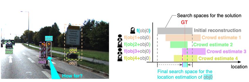
51:2                                                                                           Jean Y. Song et al.

Fig. 1. This paper introduces an approach to crowd-powered estimation of the 3D location of a target object
(here, obj0) by jointly leveraging approximate spatial relationships among other in-scene objects (obj1-obj4).
Our approach lets crowd workers provide approximate measurements of familiar objects to improve collective
performance via our novel annotation aggregation technique, which uses the spatial dependencies between
objects as soft constraints that help guide an optimizer to a more accurate 3D location estimate.

5, 32] since it can expedite the successful deployment of real-world applications, such as self-
driving vehicles [48, 50], interactive assistive robots [25, 60], or augmented and virtual reality
systems [44, 51]. This conversion of 2D to 3D typically involves collecting manual annotations,
where people provide the computers with the necessary information to bridge the gap between 2D
and 3D, e.g., pixel-level indications of where the edges of an object are. To collect these annotations
at scale, crowdsourcing is often used since it conveniently enables prompt and flexible worker
recruitment [1, 10].
   We consider the 2D to 3D object pose estimation task as a cooperative crowd-machine task where
a computational process of parameter estimation is performed based on the manual annotations
from a group of people with diverse background and knowledge. We chose to focus on the problem
of searching for a solution through an iterative optimization process because the 3D pose estimation
cannot be computed deterministically due to the many unknown parameters and the annotation
noise [2, 36, 40, 41]. Manual annotations are usually noisy and limited by the finite resolution of an
image, which results in low precision annotations due to both limited subpixel-level information
and restrictions in humans’ perceptual abilities and motor skills [58].
   Our key insight in estimating the pose of a particular target object in a 2D RGB scene is that
the joint use of annotations on multiple in-scene objects enables a more accurate solution while
providing a means of leveraging more diverse knowledge (of different objects) from groups of
people. Our approach converts crowd workers’ approximations about the reference objects (that are
near the target object) into soft constraints for an optimization algorithm that estimates the pose
of the target object. As shown in Figure 1, the crowd-generated soft constraints for the optimizer
penalize unlikely solutions and improve the chances of finding a more accurate solution. By relaxing
the accuracy requirements for each individual person, our approach also allows crowd workers
with diverse levels of knowledge to contribute to the system.
   To explore the design space of the crowd worker interface, in Section 4, we conducted an
experiment using different question formats to elicit measurement approximations of in-scene
objects. We found that annotation accuracy does not vary hugely with respect to the question
format given to the workers. Next, to understand the potential performance improvement using
the proposed annotation and aggregation approach, in Section 5, we conducted a characterization
study with a controlled experiment using a synthesized virtual dataset with absolute ground

Proc. ACM Hum.-Comput. Interact., Vol. 4, No. CSCW1, Article 51. Publication date: May 2020.
C-Reference: Crowd-Powered Joint Object Pose Estimation                                                        51:3

truth. Based on the controlled study results, in Section 6, we developed C-Reference, a crowd-
powered system that reconstructs the 3D location of a target object based on manual annotations
on target and reference objects. To demonstrate the effectiveness of the system, we recruited 339
crowd workers from Amazon Mechanical Turk to annotate 90 total objects across 15 realistic
computer-generated images of indoor and outdoor scenes. The end-to-end experimental results,
from annotation collection to 3D location estimation, show that our approach significantly reduces
the average 3D location estimation error by 40% with only 35% as much human time compared to
using single-object annotations.
   The crowd-machine hybrid method we presented in this paper could be used in other computer-
supported cooperative work (CSCW) settings by enabling human annotators to quickly provide
approximations of useful values and by allowing computers to perform precise and complex
optimization tasks using these annotations. A necessary precondition in applying our approach is
the availability of connecting annotations on different and diverse objects so that they can inform
one another. For example, in tasks such as word sentiment annotation, one can imagine collecting
annotations on diverse different, but connected, nearby words, then computationally aggregating
them to estimate characteristics of a target word of interest.
   This paper makes the following contributions:
      • We introduce a crowd-machine cooperative approach that strategically aggregates heteroge-
        neous information from multiple different objects with a shared spatial relationship to more
        accurately estimate the pose of the target object of interest.
      • We present a characterization study to demonstrate the effectiveness of our proposed approach
        via a controlled experiment with a large synthetic dataset.
      • We create C-Reference, a system that implements our proposed multi-object aggregation
        method to more accurately estimate 3D poses of objects from 2D images.
      • We report experimental results and analysis from a study using C-Reference that demonstrates
        our proposed approach can more efficiently and accurately estimate the 3D location of a
        target object compared to using single-object annotations.

2     RELATED WORK
This research draws upon prior work on designing crowdsourcing workflows to elicit diverse re-
sponses, creating aggregation techniques for combining crowdsourced annotations, and combating
challenges in 2D to 3D object pose estimation.

2.1    Eliciting Diverse Responses from the Crowd
Crowdsourcing is a powerful method for obtaining human-labeled datasets that artificial intelligence
systems using machine learning algorithms need to function. Usually, diverse responses, which are
treated as a random variable, are combined using an aggregation method to estimate the single best
label (e.g., by computing the arithmetic mean of the responses). While conventional approaches
perceive the diversity in crowd responses as errors that should be canceled out by accumulating
more responses, recent studies started to look at the diversity as a special property to be strategically
leveraged.
   In paraphrasing tasks, for example, diverse responses are encouraged because novel paraphrases
are expected, and they can be elicited by priming the annotators with different example para-
phrases [27]. Similarly, in text summarization tasks, more accurate results were achieved when
asking crowd workers to write multiple summaries covering different aspects of text compared
to one summary that includes all the key elements [26]. In entity annotation tasks, it was shown

                       Proc. ACM Hum.-Comput. Interact., Vol. 4, No. CSCW1, Article 51. Publication date: May 2020.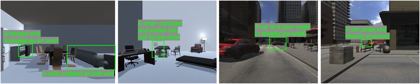
51:4                                                                                           Jean Y. Song et al.

that identifying diverse, but valid, crowd worker interpretation provides insight into sources of
disagreement [29]. Recent work shows that having each crowd worker suggest diverse answers is
beneficial in an emotion annotation task because response diversity enables the efficient construc-
tion of a large collective answer distribution [7]. Another effective diversity elicitation approach
has been demonstrated in crowd-powered GUI testing, where diverse navigation paths increase the
test coverage [6].
   Other works systematically elicit diverse responses from the crowd to obtain an accurate single
aggregated artifact. For example, using multiple tools for the same image segmentation task to elicit
different responses shows that the aggregation quality is better than using a single homogeneous
tool [56, 57]. Other research similarly finds that dynamically switching workflows for the same task
yields diverse responses that can be aggregated into a single valid answer for NLP training [39].
While these works focus on leveraging diverse responses to reduce error biases induced by the
tools or the workflows, other works leverage diverse responses as a means to compensate the
uncertainty of data [7, 58].
   The common thread behind these research efforts is that they leverage diverse responses to
increase collective information, which can reduce aggregate noise or compensate for biases when
combined appropriately. Our work contributes to this line of research by eliciting diversity in
knowledge and perspectives from the crowd in order to provide rough, but effective, relevant values
to a computational optimizer.

2.2    Aggregation Techniques for Combining Crowdsourced Annotations
Aggregation is a core aspect of crowdsourcing that ensures the quality of task results [31, 42].
Typically, diverse responses from multiple crowd workers performing the same task are aggregated
to obtain high quality annotations [38, 55]. Many aggregation techniques have been studied, rang-
ing from the majority vote [35, 55] to individually weighted data aggregation methods, such as
the expectation maximization (EM) algorithm [11, 24, 34]. Recent studies in crowdsourcing have
explored methods for aggregating heterogeneous sets of annotations to achieve even better perfor-
mance than when homogeneous sets of annotations are aggregated. We define a heterogeneous set
of annotations as a set of annotations that are not generated from an identical task setting (e.g.,
generated from different interface or different input data). In image segmentation tasks, Song et
al. [56, 57] introduced an EM-based aggregation technique, which aggregates a heterogeneous set
of responses generated by using different tools on the same task to achieve higher accuracy than
any homogeneous set of responses. In the task of reconstructing 3D pose from 2D videos, Song et
al. [58] used particle filtering-based method to aggregate heterogeneous annotations from different
video frames to assure higher annotation accuracy.
   While the idea of aggregating heterogeneous annotations of a single target object has been
explored, to the best of our knowledge, there is no experimental study on the effectiveness of
combining annotations for multiple heterogeneous objects. Our joint object annotation aggregation
introduces a new idea of aggregating annotations of multiple different objects by using the shared
spatial relationship between them. The proposed techniques enable creating soft constraints for an
optimizer, which helps find a better solution by reducing the uncertainty of the 3D pose estimation.

2.3    Challenges in 2D to 3D Object Pose Estimation Problem
Despite the great progress in computer vision on problems such as object category detection and
object 2D bounding box detection, estimating the 3D properties of objects from a single RGB image
is still a challenging problem [13, 23, 52, 64]. There have been breakthrough approaches using RGB-
D sensor, which leverage the depth information from the additional channel to estimate the 3D pose

Proc. ACM Hum.-Comput. Interact., Vol. 4, No. CSCW1, Article 51. Publication date: May 2020.
C-Reference: Crowd-Powered Joint Object Pose Estimation                                                        51:5

of objects [10, 22, 66]. However, these methods do not provide solutions when depth information is
missing, e.g., estimating 3D properties of objects shot by ordinary monocular cameras.
    Estimating 3D state from depth-less 2D images is especially challenging because the projection
operation from the 3D world to the 2D image removes a dimension of information and, as a
result, an infinite number of 3D worlds can correspond to a single 2D image [19]. As a data-driven
approach, deep learning based on convolutional neural networks (CNNs) is often used, which
requires a large number of training datasets of the target object [14, 21]. To overcome this limitation,
non-data-driven approaches have been introduced which use explicit visual cues in images, such as
object boundaries, occlusion, linear perspective, parallel line pairs, or aerial perspective [9, 45]. As
it is difficult to get these cues with machine computation only, they are usually manually annotated
with approaches such as keypoint annotations [62], bounding box annotations [18], or dimension
line annotations [58]. Also, an interesting novel approach, LabelAR [33] has been introduced, which
uses augmented reality for fast in-situ collection of images and 3D object labels for acquiring
training datasets. Since this method requires an AR-enabled camera to perform annotation tasks, it
does not scale to the general problem of converting plain 2D image to 3D.
    Manual annotation tasks often require annotators to “estimate” or “guess” contextual information
based on their perception, e.g., if an object is occluded, the worker needs to guess the hidden part to
draw a bounding box or a dimension line as accurate as possible. While this estimation process could
be challenging due to limited perception or knowledge, the annotation task could be challenging as
well, due to factors such as limited human motor skill and restricted resolution of the images. This
affects the 2D to 3D conversion performance, because the preciseness needed is often on the level
of sub-pixels. As demonstrated in Popup [58], even a single pixel noise in annotation can lead to a
few meters of error when converted into 3D.
    Even though they lack 3D information, 2D images contain rich texture information, which
can be leveraged to infer 3D spatial information (e.g., looking at other objects in the image as
a reference). While recent studies in computer vision have explored the benefit of leveraging
the texture information [18, 43, 53, 68, 71], crowdsourcing techniques for annotation task mostly
focused on looking at a single target object to be annotated, e.g., providing tools to help annotate
the target object more precisely [1, 49]. In this paper, we propose a novel annotation aggregation
method that allows annotators to estimate approximate measurements of reference objects around
a target object to help improve the performance of 3D state estimation of a target object.

3     EVALUATION METHOD
To add clarity for the remainder of the paper, we begin by describing the dataset that we use for all
of our empirical results, as well as our metrics of success.

3.1    Dataset
To evaluate our approach, we need a 2D image dataset with corresponding 3D ground truth answers.
However, we found that existing open datasets contain errors from the sensors used to capture
the scenes, and from mistakes made during the manual annotation of 3D bounding boxes [3]. For
example, Figure 2 shows the ground truth bounding box of the KITTI dataset [17], which has non-
negligible errors in their ground truth 3D bounding box annotations. We manually hand coded 140
ground truth annotations, randomly selected from the dataset, where 26.4% of the annotations were
categorized as “accurate”, 42.2% were categorized as “inaccurate”, and 31.4% were categorized as
“cannot tell”. In fact, other large-scale datasets such as Pascal3D+ [70], ObjectNet3D [69], and SUN
RGB-D [59] have also been identified as having insufficient accuracy in 3D pose annotations [67].

                       Proc. ACM Hum.-Comput. Interact., Vol. 4, No. CSCW1, Article 51. Publication date: May 2020.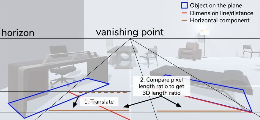
51:6                                                                                             Jean Y. Song et al.

Fig. 2. We hand-coded 140 images of ground truth 3D bounding box annotations, which were randomly
sampled from the well-known KITTI open dataset [17]. The errors of the ground truth annotations were
non-negligible, where 42.2% were categorized as inaccurate. This figure shows four examples of the incorrect
annotations.

   Therefore, instead of testing on existing datasets, we created a synthetic 3D dataset using the
Unity 3D game engine, which let us generate absolutely correct ground truths for the 3D object
pose values. We created 15 unique 2D scenes (10 indoor and five outdoor scenes) with absolute
3D ground truths of all objects’ position values, dimension values, and the 2D pixel values. The
resolution of each image we synthesized was 2880 × 1800 pixels. For each image, we selected one
target object at random to be estimated. Next, we arbitrarily choose five reference objects for each
test image. We assume that no information (size, type, etc) is known by the requester or crowd
workers for these reference objects. To demonstrate the robustness of our approach, we include
objects that are small, heavily occluded (more than 50% occluded), or have a limited view angle
from the camera’s perspective. Examples of these challenging-to-annotate objects are shown in
Figure 3. We report the performance of the object pose estimations in Section 7. We observed that
the quality of estimation results are approximately uniform across object types. To show the scope
of our synthesized dataset, we included the characteristics of the scenes and objects in Table 1.

       Number of scenes            10 indoor scenes and 5 outdoor scenes
       Type of scenes              4 types of indoor scenes: bedroom, living room, kitchen, bathroom
                                   1 type of outdoor scene: outdoor street
       Type of objects             19 types of indoor objects: bookcase, dining table, coffee table, office
                                   desk, chair, couch, sink, fridge, mirror, stand, acoustic system, bed, etc
                                   9 types of outdoor objects: vehicle, hydrant, traffic sign, bush, bench,
                                   chair, trash basket, etc
       Objects’ range of distance 2.25 to 45.48 meters
       Objects’ range of height    0.24 to 3.82 meters
       Objects’ range of length    0.025 to 4.63 meters
       Objects’ range of width     0.06 to 5.24 meters
                                 Table 1. Summary of our synthesized dataset

3.2     Metrics
To assess the quality of intermediate and final output of our system, we use percentage error to
represent deviation from the ground truth value. We used percentage error instead of absolute
measurement error because the same absolute measurement error can mean different severity of
errors with respect to the target object, e.g., 0.5 meter measurement error for a chair’s length can
be a severe error, but the same absolute measurement error would trivial for the length of a train. If
the output is a range, we also measure precision.

Proc. ACM Hum.-Comput. Interact., Vol. 4, No. CSCW1, Article 51. Publication date: May 2020.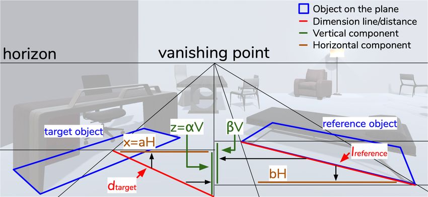
C-Reference: Crowd-Powered Joint Object Pose Estimation                                                        51:7

                 Fig. 3. Examples of challenging objects in our synthesized image dataset.

Percentage Error:
  If the output is a scalar value, we compute the percentage error as follows:
                                                 |m̃ − GT|
                                           errs =            × 100                            (Eq. 1)
                                                     GT
where m̃ is the estimate value, GT is the ground truth value, and | · | indicates absolute value.
   When the output value is a range with scalar valued bounds, we use a slightly modified formula-
tion as follows:
                                         |(m̃ L + m̃ U )/2 − GT|
                                   err =                         × 100                        (Eq. 2)
                                                    GT
where m̃ L is the lower bound of the output range and m̃ U is the upper bound of it, which measures
the percentage error; this measure assumes that the value is at the center of the given range.
   If the output is a vector value, we compute the percentage error as follows:
                                                  ||m̄ − GT||2
                                         errv =                × 100                                       (Eq. 3)
                                                     ||GT||2
where m̄ denotes the estimated 3D location vector, GT denotes the ground truth 3D location vector,
and || · ||2 denotes Euclidean distance.

Precision:
  When the output value is in range, the precision of the range is computed as follows:
                                                     (m̃ U − m̃ L )
                                     precision =                     × 100                                 (Eq. 4)
                                                    (m̃ L + m̃ U )/2
where m̃ L and m̃ U are lower and upper bounds of the range, respectively.
  Note that for both percentage error and precision, a lower value means better performance.

4   WORKER INTERFACES FOR OBJECT MEASUREMENT APPROXIMATION
This section explores different formatting conditions for the approximate object measurement
annotations. There are multiple ways to design an annotation interface, which we explore along
three dimensions: annotation selection, annotation directness, and annotation granularity. The
findings from this section shows that regardless of the design of the annotation interface, crowd
workers’ annotation accuracy is similar. Each interface asks annotators to draw the corresponding
length lines on the reference objects, as shown in Figure 4(c). We explore diverse formatting
conditions of measurement estimates to understand trade-offs in crowd worker performance
(accuracy and precision) when generating different measurement approximations.

                       Proc. ACM Hum.-Comput. Interact., Vol. 4, No. CSCW1, Article 51. Publication date: May 2020.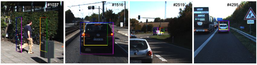
51:8                                                                                           Jean Y. Song et al.

4.1     Formatting Conditions of Measurement Estimate Annotation
Providing various options for the formats of measurement estimate annotation helps facilitate
the use of varied knowledge of the size and dimensions of different objects from crowd workers.
While measurement estimates of reference objects can be asked and can be answered in a wide
range of formats, we explored three different dimensions in designing the input format for the
measurement estimates: selection (length of an object, width of an object, or distance of an object
from the camera), directness (direct measurement of an object or relative measurement compared
to another object), and granularity (single valued answer or range valued answer). We chose these
three conditions because they are orthogonal and thus can be combined (e.g., annotating the length
of an object via a range that is relative to a different object’s length).

4.1.1 Selection of Measures. While our annotation aggregation method can make use of any line
drawn on the ground and its corresponding actual measurement value, it is hard for humans to
estimate the actual measurement value of a line if there is no visual reference. Therefore, we asked
workers to annotate lines that have visual object reference points in the scene. We asked them to
annotate the length and width of in-scene objects that can be estimated based on prior exposure to
and knowledge about everyday objects (e.g., the length of a table is usually greater than that of a
chair). Our approach projects these annotations onto a share reference plane (any reference plane
could be used without loss of generality), which in this study, was chosen to be the ground plane of
the scene. Among the three dimension of an object, width, length, and height, we did not asked to
annotate height because it would be orthogonal to our selected reference plane. We did not include
height measurements of objects since they cannot be drawn on the ground. Each object’s distance
from the camera can be inferred based on the scene in a given image, e.g., if there are three cars in
a row, one can tell approximately how far the last car is from the camera. Example measurement
estimates are:
       • Lenдth: The object is about 165 inches long.
       • W idth: The object is about 50 inches wide.
       • Distance: The object is about 35 feet away.

   Note that because the camera location is not visible from the image, instead of asking the distance
from the camera, we designed the interface to ask crowd workers to consider the distance “from
the bottom of the image”. In the instructions, we provided example GIF images that demonstrate
how to draw length lines to help workers understand the task.

4.1.2 Directness of Measures. Depending on the context, sometimes it can be easier to estimate
a relative measurement than the direct measurement of an object. This is especially true when
the object is not familiar to the annotator, because people naturally use prior knowledge of other
objects to infer the properties of a new object [20, 61]. Therefore, we implemented both an interface
to input direct measurements as well as relative measurements. However, if we let crowd workers
make the inference based on any object in the task image, it becomes hard for the computer to
aggregate the annotations, because the computer does not know the true measurements of the
other objects. Therefore, we restricted this comparison to be done only with the target object to be
reconstructed, which we already know the exact true size of. Example measurement estimates are:
       • Direct: The object’s length is about 80 inches.
       • Relative: The object is about 10% longer than the target object.

Proc. ACM Hum.-Comput. Interact., Vol. 4, No. CSCW1, Article 51. Publication date: May 2020.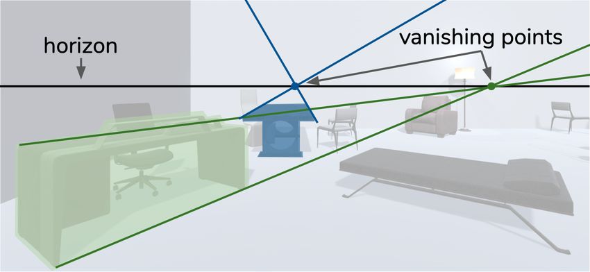
C-Reference: Crowd-Powered Joint Object Pose Estimation                                                        51:9

Fig. 4. The interactive worker UI is comprised of three steps in which workers approximate object mea-
surements and annotate dimension lines. (a) The instructions and task image step: the reference object
to be annotated is marked with a green box. If the relative condition is assigned, the UI also provides an
indication of the target object (red box). However, for the workers, we reversed the name of the objects,
since the reference object for the optimizer is the target to manually annotate for the workers. (b) The
measurement-approximation step: each worker sees different instructions based on the condition they are
assigned. (c) Length line annotation step: crowd workers were instructed to draw the line that represents the
measurement they provided in the second step.

4.1.3 Granularity of Measures. Unless the annotator knows the exact make and model of an
object, it is infeasible to precisely identify the length or width of it. Similarly, for the distance
measurement, it is hard to tell the exact distance of an object from a single image. Therefore, we
designed two elicitation approaches, a single valued estimate and a ranged valued estimate. For
the range valued approach, the annotators can freely choose the granularity of their answer. Our
proposed joint object annotation aggregation method can handle multiple granularities because
the penalty function (Eq. 6) is designed to accept lower and upper bounds. Example measurement
estimates are:
    • Sinдle: The target is about 32 feet away.
    • Ranдed: The target object is about 30 feet to 40 feet away.

  Even though there are 12 possible combinations of measurement estimation formats (3 selection
× 2 directness × 2 granularity), we used 10 formats in the study because without at least one absolute
measurement for the distance selection, the system of equation becomes under-constrained with
no absolute solution. Therefore, we excluded the two combinations distance × relative × sinдle
and distance × relative × ranдed from both the interface design and the data collection.

                       Proc. ACM Hum.-Comput. Interact., Vol. 4, No. CSCW1, Article 51. Publication date: May 2020.
51:10                                                                                               Jean Y. Song et al.

        (a) Different selection              (b) Different directness               (c) Different granularity

Fig. 5. Cumulative frequency of annotation is plot with respect to percentage error of the annotation. No
significant difference was observed within each dimension.

                                        length                      width                      distance
         direct × single          61.98/120.43(180.05)       60.65/64.21(57.77)        51.02/60.09(61.84)
         direct × range           67.31/167.56(270.63)      61.94/184.46(698.51)       49.88/55.15(49.19)
         relative × singe         65.24/238.02(658.27)      65.02/109.38(151.22)               -
         relative × range         58.51/291.16(1209.50)     68.01/104.58(129.45)               -

Table 2. Median/Average(Standard Deviation) percentage error computed as in Eq. 1 and Eq. 2 to evaluate
worker answers for different measure input formatting conditions.

4.2 Task Interface
Our task interface presents crowd workers with step-by-step instructions and web annotation
tools. After reading through the instructions, crowd workers can proceed to the task. Then they are
shown an image with reference objects to be annotated, which are indicated with a green box. For
the relative condition, the target object to be compared is also indicated with a red box. To avoid
confusion, we note that the terminologies were reversed for the crowd workers, the UI calls target
object as reference object and vice versa, because the reference object for the computer (optimizer)
is actually a target object for the workers to manually annotate. After checking the task image, the
next step is to provide estimated measurement values, as in Figure 4(b). The workers are allowed to
choose a unit of measurement from the following four options: meters, feet, inches, and yards. The
last step is to mark the corresponding line on the selected reference object, as in Figure 4(c). Since
the length and width of an object can be ambiguous in certain cases, e.g., when an object has no
apparent longer side, we set a rule to distinguish between length and width. The rule is explained
in the instructions with various example objects as in Figure 4(b). For distance estimate annotation,
these instructions were hidden. The instructions in Step 2 included examples of corresponding
lines, and we reminded workers that the line should be drawn on the ground in the image where
the objects are positioned.

4.3     Evaluating the Impact of Measure Input Format
To evaluate the impact of measurement input format on workers’ annotation accuracy, we recruited
300 crowd workers. We asked the workers to annotate the 15 task images, 10 indoor and five

Proc. ACM Hum.-Comput. Interact., Vol. 4, No. CSCW1, Article 51. Publication date: May 2020.
C-Reference: Crowd-Powered Joint Object Pose Estimation 51:11
length width distance
direct × range 25.00/28.98(17.32) 28.57/31.09(21.48) 28.57/36.66(24.08)
relative × range 18.18/25.82(27.38) 22.22/30.62(29.64) -
Table 3. Median/Average(Standard Deviation) precision computed as in Eq. 4 to evaluate worker answers for
different measure input formatting conditions.
outdoor images, using the 10 different measurement formatting conditions. Images were grouped
into fives to distinguish indoor and outdoor images. The order of the images within a group and
the objects within an image were randomized to avoid learning effects. Each worker annotated one
object per image using a single measurement format that was given. Participants were limited to
workers from the US who had a task acceptance rate ≥ 95%. Each worker could only participate
once, and was paid $1.35 per task, yielding an average wage of $9/hr—above the 2019 U.S. federal
minimum wage.
4.4 Results
A total of 1500 annotations were collected across the 10 formatting conditions, but 18 annotations
were dropped due to task submission errors. Figure 5 shows the cumulative frequency of the
percentage error for each element within each dimension. The trend is similar across conditions: a
steep increase until 100 percent error, and then slows down.
The median and average percentage error of crowd workers’ responses for the 10 measurement
formatting conditions are shown in Table 2. To compare the performance of the 10 measurement
conditions, we ran 102 = 45 (10 choose 2) pairwise comparisons using a Mann-Whitney U test be-
cause the worker responses were skewed (non-normal). With Bonferroni correction, we considered
the comparison result significantly different if the p-value was below .05/45 = .0011. From the 45
comparisons, the pairs with significant difference were the following four:
✓ distance×direct×range outperformed length×direct×range
(U = 8554.0, n 1 = 150, n 2 = 150, and p < .0005)
✓ distance×direct×single outperformed length×direct×range
(U = 8658.0, n 1 = 150, n 2 = 150, and p < .0005)
✓ distance×direct×range outperformed width×relative×range
(U = 8658.0, n 1 = 150, n 2 = 149, and p < .001)
✓ distance×direct×single outperformed width×relative×single
(U = 8658.0, n 1 = 150, n 2 = 145, and p < .0001)
The results show that overall crowd workers performance were similar across different formatting
conditions, but direct distance estimations significantly outperformed some of the other conditions.
The median and average precision of crowd workers’ responses for the five measurement
conditions are shown in Table 3. All sinдle estimation answers were ignored because precision is
always 0 for a single value. To compare the performance of the five measurement conditions, we
ran 52 = 10 (5 choose 2) pairwise comparisons using a Mann-Whitney U test because the worker
responses were skewed (non-normal). With Bonferroni correction, we considered the comparison
Proc. ACM Hum.-Comput. Interact., Vol. 4, No. CSCW1, Article 51. Publication date: May 2020.51:12 Jean Y. Song et al.
length width distance
absolute × raw 47.31/67.24(68.02) 44.77/56.05(43.48) 36.36/46.77(33.76)
absolute × range 45.97/62.63(53.54) 50.95/67.78(49.17) 37.48/58.21(72.93)
relative × raw 39.25/54.31(40.28) 46.45/71.61(117.76) -
relative × range 53.78/85.37(139.65) 53.30/73.97(64.30) -
Table 4. Median/Average (Standard Deviation) task time for different measure input formatting conditions.
result significantly different if the p-value was below .05/10 = .005. From the 10 comparisons, the
pairs with significant difference were the following five:
✓ length×relative×range outperformed length×direct×range
(U = 8296.5, n 1 = 150, n 2 = 150, and p < .0001)
✓ length×direct×range outperformed distance×direct×range
(U = 9007.0, n 1 = 150, n 2 = 150, and p < .005)
✓ length×relative×range outperformed width×direct×range
(U = 8658.5, n 1 = 150, n 2 = 153, and p < .005)
✓ length×relativetimesrange outperformed distance×direct×range
(U = 6562.0, n 1 = 150, n 2 = 150, and p < .0001)
✓ width×relative×range outperformed distance×direct×range
(U = 8399.5, n 1 = 149, n 2 = 150, and p < .0005)
The results show that workers tend to provide a narrower range when asked to annotate the
relative measurement conditions. We also report the task time difference in Table 4, which did not
significantly differ across formatting conditions. Overall, the average accuracy and precision of
worker annotations were similar across different formatting conditions, even though there were
some cases with significant performance differences. While images may contain various different
objects in varying contexts, providing workers with as many different ways for them to provide
estimates as possible will allow to cover the diverse cases of use, maximizing the benefit of diverse
knowledge among workers.
5 C-REFERENCE: JOINT OBJECT 3D LOCATION ESTIMATION
In this section, we introduce our proposed joint object estimation method, which estimates the
3D location of a target object using diverse sets of 2D annotations from other objects in the scene.
Our approach transforms the approximate size or distance measurement annotations of multiple
objects to soft constraints that are then used by an optimizer, making it possible to use multiple
levels of measurement granularity. This enables our C-Reference system to leverage heterogeneous
information in a way that collectively generates more accurate system output than using a single
object.
5.1 Naive Iterative Optimization for Estimating the 3D Location of a Target Object
For 3D location estimation, we build on the method from Popup [58], which estimates the 3D pose
of a target object using three “dimension line” (length, width, and height of an object) annotations
drawn on 2D images. Dimension lines provide richer information compared to other annotation
Proc. ACM Hum.-Comput. Interact., Vol. 4, No. CSCW1, Article 51. Publication date: May 2020.C-Reference: Crowd-Powered Joint Object Pose Estimation 51:13
methods. Specifically, they can be used to determine both 3D location and orientation information
of an object, while keypoint annotation [62] can only provide orientation information and 2D
bounding boxes [18] can only provide location information.
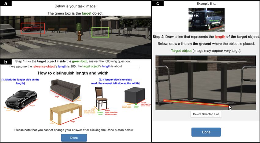
The three dimension lines, as shown inside the white box in Figure 6, create four corners (c 1 , c 2 , c 3 ,
and c 4 ), which is used to convert the problem of 3D location estimation to a perspective-n-point
problem [16, 37], where the intrinsic camera parameters are unknown and the manual annotations
are noisy. As in Popup [58], we assume that the target object as well as the dimensions of it are
known, and the objective is to determine the orientation and location of the target object in 3-space.
5.1.1 Designing the Baseline Cost Function.
We estimate five unknown variables, x, y, z, θ, and µ, using the four corners of dimension line
annotations of a target object. Here, x, y, z are the 3D location of the target object (x and z along
the ground plane, where z is the depth from the camera, and y being the normal (perpendicular)
direction from the ground plane), θ is the yaw-orientation of the object, and µ is the camera
focal length. The corners of dimension line annotations are input to an iterative optimizer, which
we implemented based on the L-BFGS-B algorithm [58, 72]. While any iterative computational
optimization method can be used for our application [30] (e.g., Newton’s method or Nelder-Mead
method), we chose L-BFGS-B within scipy.optimize.minimize library [28] because it enables us
to set bounded constraints and is known to be memory-efficient [15]. We applied a basin-hopping
technique [65] to iterate multiple times with random initialization, only accepting a new solution
when its cost is minimal along all the candidate solutions visited during the iteration. The objective
function to be minimized is designed as follows:
4
!
2
Õ
cost(s, µ) = − log(f (||t i − C µ (x s )i ||2 ; 0, σ )) + ||t i ||2 − ||C µ (x s )i ||2 (Eq. 5)
i=1
where the optimizer finds s̄, µ̄ = argmin(cost(s, µ)). Here s̄ denotes the estimated 3D pose, µ̄ denotes
{s ∈S, µ }
the estimated camera focal length, s denotes one of the 3D pose candidates, S denotes all valid 3D
pose candidates, and µ denotes one of camera focal length candidates. In Eq. 5, f (w; 0, σ ) denotes
the probability density function of a normally distributed random variable w with a mean of zero
and standard deviation σ , t i denotes one of the four corners from a set of dimension lines, i denotes
the index of each corner, C µ (·) denotes the camera projection matrix with focal length µ, and x s
denotes the 3D bounding box of the target object for pose s based on x, y, z. Lastly, || · ||2 denotes the
Euclidean distance and | · | denotes absolute value. Note that we did not use the particle filter-based
method proposed in Popup [58] because it is not applicable to static images.
5.1.2 Limitations of Using the Baseline Cost Function.
While the optimizer is designed to find the minimum cost of the objective function, there are a
few factors that can cause poor estimation results. First, annotation noise in the dimension lines can
affect the estimation result. Even a small discrepancy (e.g., smaller than five-pixel error in 2D) in
the annotation accuracy can lead to a significantly amplified error (e.g., larger than 20-meter error
in 3D) in the estimation result depending on the camera parameters [58]. Unfortunately, collecting
super-precise visual annotations on 2D images is challenging because of factors such as limited
human motor precision, limited pixel resolution, and limited human visual perception. Second, while
the optimizer can find the global optimum in cases where input annotations have zero noise and the
initial values are set at the global optimum, in other cases it fails to find the global optimum, instead
finding local optima as a solution, making the performance highly dependent on the initial values
chosen. To resolve the local minimum problem, more information such as additional constraints
for the search area can be added to the optimization process to help avoid searching near infeasible
Proc. ACM Hum.-Comput. Interact., Vol. 4, No. CSCW1, Article 51. Publication date: May 2020.51:14 Jean Y. Song et al.
Fig. 6. A test image with known ground truth of objects. Inside the white bounding box is the target object
(a cupboard) to be estimated. Three colored line on the object represents the ground truth dimension lines,
length (L), width (W), and height (H). Green lines ( 1 , 2 , and 3 ) are the reference object annotations.
solutions. In the next section, we introduce a novel annotation aggregation approach that helps the
optimizer overcome these limitations by generating additional soft constraints from even rough
and less precise annotations.
5.2 Proposed Joint Object Annotation Aggregation
To achieve better estimation results that overcome limitations from pixels and local optima, we
introduce an approach that guides a better search area using soft constraints that are generated from
diverse crowd annotations on multiple objects. The key insight is that having multiple objects will
allow crowd workers to use their diverse knowledge about familiar objects and not have to rely on
a single source of information when annotating. To combine the heterogeneous annotations from
different objects/sources, we first introduce a penalty function that is generated by merging multiple
soft constraints. The advantage of converting the annotations into soft constraints is that the
accuracy requirement for usable annotations can be relaxed, allowing even rough approximations
to contribute to the system performance. Next, we introduce a novel aggregation method that uses
the shared spatial relationship among the objects to unify and transform the annotations into a
useful input value for the penalty function.
5.2.1 Designing a Penalty Function.
We introduce a penalty function that creates a soft constraint for the optimizer using approximate
search bounds. The soft constraints penalize the optimizer for selecting an unlikely solution and
encourages finding a better solution, ideally near the ground truth. We design a penalty function
based on a weighted sigmoid function which penalizes x if x is below l or above u as follows:
P(x) = S(l − x) + S(x − u) (Eq. 6)
where S(x) is the weighted sigmoid function with a weight x + 1,
!
x +1
S(x) = max ,M (Eq. 7)
(1 + e −ax )
Proc. ACM Hum.-Comput. Interact., Vol. 4, No. CSCW1, Article 51. Publication date: May 2020.C-Reference: Crowd-Powered Joint Object Pose Estimation 51:15
and l is a lower bound, u is an upper bound, a is the (curve) sharpness parameter, and M is a
threshold to prevent the penalty function from dominating the objective function. While the two
parameters a and M can be arbitrarily tuned, the additional information of l and u is best chosen
to be near the ground truth so that the penalty function can narrow down the search area for
the optimizer. In the next section, we design and introduce a joint object annotation aggregation
method, which aggregates approximate annotations from different reference objects—all other
objects in the scene except the target object—to obtain reasonable values for both l and u.
5.2.2 Annotation Aggregation Method.
As input, the proposed annotation aggregation approach uses (i) 2D line annotations of the size
of reference objects and distance of those objects from the camera and (ii) measurement values for
those lines as in Figure 4. The goal of this annotation aggregation is to approximate the position of
the target object relative to the camera position (x and z optimized in Eq. 5), and to use it as the
search bound for the soft constraint (l and u in Eq. 6). With this goal, our proposed aggregation
approach utilizes the spatial relationship between the reference objects and the target object, which
is possible because they share the same ground plane and vanishing points, to transform the 3D
properties of the reference objects into the pose estimation of the target object. This setting enables
us to make use of the 3D affine measurements even with a single perspective view of a 2D scene,
given only minimal geometric information (e.g., vanishing points and horizontal line) from the
image [8].
Specifically, our goal is to find the position of the target object relative to the camera, which
can be represented as x and z that are optimized in the cost function (Eq. 5). To get these values,
we use the following four pieces of information: (i) the line between the target object and the
camera drawn on the 2D task image (dt ar дet in Figure 7(b)), (ii) two lines from two reference objects
(one from each object) in the 2D task image, which represent the length, width, or the distance
from the camera (lr e f er ence in Figure 7(b)), (iii) the approximation of the reference lines’ actual
measurements, and (iv) the horizon in the 2D image, obtained from the connection of vanishing
points (Figure 7(a)). The center of the target object’s bottom, dt ar дet , is computed from the target
object’s dimension lines. The horizontal and vertical component of dt ar дet is x and z, respectively.
The horizon can be estimated using off-the-shelf computer vision algorithms [12, 63] or it can be
obtained manually. As shown in Figure 7(a), we assume that both the reference objects and target
object share the same ground plane and vanishing points. This is reasonable because objects are
place on the same plane for many of use cases such as reconstructing outdoor driving scenes.
To get approximate values of x and z, we solve equations for length relations between dt ar дet
and lr e f er ence in real-world 3D space for all lr e f er ence . For lr ef er ence , we first decomposed x and z
into vertical and horizontal components as in Figure 7(b), since horizontal and vertical components
have different characteristics when they are projected from 3D to 2D. After decomposition, for each
of horizontal and vertical components, we calculate the length ratio between the components from
dt ar дet and that from lr e f er ence . The length of each component is denoted by multiplying the ratio
and the unit lengths (V and H ) for vertical component and horizontal component, respectively.
Using the length ratio, we can set the following equation with one reference object line annotation:
(dt ar дet )2 = (aH )2 + (αV )2 (Eq. 8)
(lr e f er ence )2 = (bH )2 + (βV )2 (Eq. 9)
Here, a and b are constants calculated from the ratio of the horizontal component length of dt ar дet
and lr e f er ence , and α and β are constants calculated from the ratio of the vertical component length
of those two. As stated before, V and H are unit lengths for vertical and horizontal components.
Proc. ACM Hum.-Comput. Interact., Vol. 4, No. CSCW1, Article 51. Publication date: May 2020.51:16 Jean Y. Song et al.
(a) Horizon line and vanishing
point obtained using the scene
features.
(b) Aggregation Step 1: decom-
pose the virtual line to the
target object’s center (dt ar дet )
and the annotation line of the
reference object (lr ef er ence )
into vertical (along the vanish-
ing point) and horizontal (par-
allel to the horizon) compo-
nents.
(c) Aggregation Step 2: find the
four points along the vertical
line from camera center to a
vanishing point to conduct the
cross-ratio based computation,
using either 1 or 2 .
(d) Aggregation Step 3: use
the cross-ratio based computa-
tions ( 1 and 2 in (b)) to map
the decomposed components’
length in real-world with the
crowd workers’ measurement
estimation annotations.
Fig. 7. Step-by-step aggregation of reference object annotations using cross-ratio and vanishing points.
Proc. ACM Hum.-Comput. Interact., Vol. 4, No. CSCW1, Article 51. Publication date: May 2020.C-Reference: Crowd-Powered Joint Object Pose Estimation 51:17
Fig. 8. Overview of the pipeline of our prototype application, C-Reference, which estimates the 3D location
of a target object using a novel joint object estimation approach. The additional information from the joint
object annotations ( 1 ) is aggregated ( 2 ) and transformed into a soft penalty function ( 3 ), allowing diverse
granularity of approximate annotations to contribute to improving the system performance.
While a, b, α, and β can be calculated from the 2D task image, dt ar дet , V , and H are unknown
variables. With two reference object annotations, we can set one equation for the target object (Eq.
8) and two equations for reference annotations (Eq. 9), which share the unknown variables. Then
we can solve the equation problem for these unknown variables. With solved V and H , we can find
x and z, which are αV and aH , respectively.
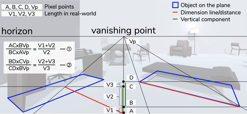
To obtain the ratio of vertical components between two lines, we used a cross-ratio, which is
the ratio between four points on the same straight line as in Figure 7(c). Because a cross-ratio has
a projective invariant property, where the ratio in projected pixels and lengths in the real-world
3D space are the same (since cross-ratios are invariant to perspective projection), we can use it to
compute the length ratio of lines in the real-world 3D space. For instance, in 1 of Figure 7(c), the
2D line AC corresponds to 3D real-world length V 1 +V 2, and BC to V 2. As the 2D line BVp and AVp
have the length of infinity in 3D real-world space, we can consider these lines have equal length
in real-world, and the cross-ratio equation for point A, B, C, and Vp would be as 1 . The same
projective invariant property also applies to 2 , and with these two equations, we can calculate 3D
real-world length ratio between V 1, V 2, and V 3, which enables us to calculate α and β.
For the ratio of horizontal components between two lines, we first translate the decomposed
horizontal component so the sub-components are on the same straight line parallel to the horizon
as in Figure 7(d). The reason is because lengths of horizontal components can be compared as
the real-world 3D length only when they are at the same vertical distance from the camera. After
the translation, we compute the length ratio of the two horizontal components with the ratio of
the pixel length. This ratio is same as the ratio of the 3D real-world length of line aH and bH ,
which enables us to calculate a and b. If the annotations contain parallel line (either correctly or
incorrectly), then the system of equations from Eq. 8 and Eq. 9 will have no solutions. In this case,
we do not input this in the penalty function to avoid unrealistic penalty function.
5.3 C-Reference
Based on the proposed joint object annotation aggregation method, we implemented C-Reference,
a crowd-powered 3D location estimation system that leverages approximate annotations from the
reference objects to more accurately estimate the 3D location of a target object. Figure 8 shows the
system pipeline of C-Reference.
Proc. ACM Hum.-Comput. Interact., Vol. 4, No. CSCW1, Article 51. Publication date: May 2020.51:18 Jean Y. Song et al.
The penalty function we designed (Eq. 6) is integrated into the objective function (Eq. 5) as
follows: Õ
cost′ = cost + Pi j (x s ) (Eq. 10)
i, j ∈R
where cost is the objective function in Eq. 5, R is a set of reference object annotations, and
Pi j (x s ) = S(di j,l − x s ) + S(x s − di j,u ) (Eq. 11)
where S(·) is the weighted sigmoid function described in Eq. 7, di j is dt ar дet approximated from
reference object annotations i and j. Finally, l and u are the lower and upper bounds of the
approximation of di j . Because the penalty function can accept lower and upper bounds, it is
possible to leverage the approximate measurement of objects at any level of granularity.
6 CONTROLLED STUDY OF SIMULATED ANNOTATION ERROR
To verify the feasibility of our aggregation method, we conducted two controlled studies with
simulated data points that allows us to obtain absolute ground truths. This way, we were able
to systematically control the annotation and measurement errors and investigate the system
performance with respect to the level of input error. We first investigate the performance of module
3 in Figure 8 without the additional information from the penalty function. Next, we investigate
the performance of our joint object aggregation method (module 2 in Figure 8) which generates
the input to the penalty function.
6.1 Parameter Settings
In Eq. 5, σ was set to 100, which was heuristically selected based on the feasible solution region.
The basin-hopping iteration (random restart) number was set to 100, which was chosen by manual
parameter sweeping in a preliminary study. We picked a large number of iterations to improve the
overall performance for every condition including the baseline. There is a trade-off between accuracy
and speed when setting this parameter, which means that a larger number of iterations will improve
accuracy along with computational cost. The optimizer stopping criteria was set to 10−8 , which we
observed was reasonable for the types of scenes explore in this paper (i.e., scenes containing objects
in the order of meters in size and distance from the camera). The optimizer will converge when
the following condition meets for the stopping criteria: (s k − s k +1 )max {|s k |, |s k +1 |, 1} ≤ stopping
criteria.
If the number is too large, there is a risk that the optimizer stops before converging. The optimizer
bounds were set as −10 ≤ x ≤ 10, −10 ≤ y ≤ 10, 1 ≤ z ≤ 100, −π ≤ θ < π , and 100 ≤ µ ≤ 2000.
The bounds for the location parameters were selected based on a feasible search area. For example,
we bound the y value, which defines the distance between the bottom of the object and the ground,
to −5 < y < 5. This is because the images that we will be looking at contain objects that are
expected to be placed approximately at ground level. The bound for the unknown orientation
parameter was selected to ensure the uniqueness of the orientation solution (since 90◦ could be any
of π /2 + 2 ∗ i for any integer i). The focal length bound was selected to include typical focal lengths
of commercially manufactured cameras. For the penalty function in Eq. 7, the two parameters
were set as a = 8 and M = 50. These were selected based on the desired sharpness of the sigmoid
function and the desired size of the penalty that we want to give to the values outside the feasible
solution region. For example, if M is too large, the penalty function could dominate the objective
function, which is not desired. Lastly, we manually obtained the horizontal line using parallel lines
on the ground plane.
Proc. ACM Hum.-Comput. Interact., Vol. 4, No. CSCW1, Article 51. Publication date: May 2020.You can also read