Multi-Scale Proper Orthogonal Decomposition of Complex Fluid Flows
←
→
Page content transcription
If your browser does not render page correctly, please read the page content below
Under consideration for publication in J. Fluid Mech.                                     1

                                                           Multi-Scale Proper Orthogonal
                                                        Decomposition of Complex Fluid Flows
arXiv:1804.09646v3 [physics.flu-dyn] 4 Sep 2018

                                                               M.A. Mendez1 †, M. Balabane2 and J.-M. Buchlin1
                                                                             1
                                                                             von Karman Institute for Fluid Dynamics,
                                                                     Environmental and Applied Fluid Dynamics Department
                                                               2
                                                                 Laboratoire Analyse, Géométrie et Applications, Université Paris 13,

                                                                                 (Received xx; revised xx; accepted xx)

                                                  Data-driven decompositions are becoming essential tools in fluid dynamics, allowing
                                                  for identifying and tracking the evolution of coherent patterns in large numerical and
                                                  experimental datasets. In this work, we analyze the limits of two popular decomposi-
                                                  tions, namely the Proper Orthogonal Decomposition (POD) and the Dynamic Mode
                                                  Decomposition (DMD), and we propose an alternative which allows for superior feature
                                                  detection capabilities. This novel approach, referred to as Multiscale Proper Orthogonal
                                                  Decomposition (mPOD), combines Multiresolution Analysis (MRA) with a standard
                                                  POD. Using MRA, the mPOD splits the correlation matrix into the contribution of
                                                  different scales, retaining non-overlapping portions of the correlation spectra; using the
                                                  standard POD, the mPOD extracts the optimal basis from each of these scales. After
                                                  introducing a matrix factorization framework for data-driven decompositions, the MRA is
                                                  formulated via 1D and 2D filter banks for the data and the correlation matrix respectively.
                                                  The validation of the mPOD, and a comparison with the Discrete Fourier Transform
                                                  (DFT), DMD and POD, are provided in three test cases. These include a synthetic
                                                  test case, a numerical simulation of a nonlinear advection-diffusion problem, and an
                                                  experimental data provided by the Time-Resolved Particle Image Velocimetry (TR-PIV)
                                                  of an impinging gas jet. For each of these examples, the decompositions are compared in
                                                  terms of convergence, feature detection capabilities, and time-frequency localization.

                                                  1. Introduction and Motivation
                                                     The analysis of turbulent flows hinges upon the identification of coherent flow features
                                                  out of seemingly chaotic data. These structures could produce dynamic force loads
                                                  (Barrero-Gil et al. 2012; Rahmanian et al. 2014), unstable patterns in the evolution
                                                  of hydrodynamic instabilities (Charru & de Forcrand-Millard 2009; Gudmundsson &
                                                  Colonius 2011; Melnikov et al. 2014; Schmid & Brandt 2014), transition to turbulence
                                                  (Hussain 1986; Grinstein & DeVore 1996), enhancement of heat and mass transfer
                                                  (Mladin & Zumbrunnen 2000; Kuhn et al. 2010), noise generation (del Castillo-Negrete
                                                  et al. 2008; Nagarajan et al. 2018) and more.
                                                     The development of data processing algorithms for detecting coherent features is con-
                                                  tinuously fostered by the availability of datasets with ever-growing resolutions, and by the
                                                  big data revolution with permeates any area of applied science. Identifying the relevant
                                                  features from high-dimensional datasets is the purpose of data-driven decompositions,
                                                  which lay the foundation of model order reduction (MOR), data compression, filtering,
                                                  pattern recognition and machine learning, and which are nowadays greatly enlarging the
                                                  toolbox at the researcher’s disposal. Recent reviews on data-driven decomposition with
                                                                       † Email address for correspondence: mendez@vki.ac.be
2                                  M. A. Mendez et al
emphasis on fluid dynamics are proposed by Taira et al. (2017) and Rowley & Dawson
(2017); an extensive overview on the impact of the big data revolution in turbulence
research is presented in by Pollard et al. (2017), while Duriez et al. (2017) presents an
overview of Machine Learning methods for flow control.
   Data-driven decompositions represent the data as a linear combination of basis ele-
ments, referred to as modes, having spatial and temporal structures with a certain energy
contribution. These decompositions can be classified into two major classes: energy-based
and frequency-based. This work presents a generalized formulation of both approaches,
analyzes their respective limits, and proposes a novel hybrid method which combines the
advantages of the two.
   Section §2 presents a literature review on these decompositions, including recent
developments on hybrid methods, while section §3 introduces a common matrix fac-
torization framework. This framework is extensively used in Section §4 to derive a new
decomposition, referred to as multi-scale Proper Orthogonal Decomposition (mPOD).
Its performance is compared to that of other classical decompositions on an illustrative
synthetic test case (§5), a numerical test case (§6) and an experimental test case (§7).
Finally, Section §8 presents the conclusions and perspectives for the future.

2. Energy optimality or Spectral Purity?
   The fundamental energy based decomposition is the Proper Orthogonal Decompo-
sition (POD). This decomposition originates from the Karhunen Loéve (KL) theorem
(Loève 1977), which formulates the optimal (in a least-square sense) representation of
a stochastic process as a series of orthogonal functions with random coefficients. This
decomposition has set the basis for a multitude of modern data processing methods
which are known, depending on the field, as Principal Component Analysis (PCA),
Model Order Reduction (MOR), Hotelling Transform, Empirical Orthogonal Function
(EOF) or Proper Orthogonal Decomposition (POD). Literature reviews on these different
applications of the KL theorem can be found in the work of Cordier & Bergmann (2013),
and the monographs from Jackson (1991) and Holmes et al. (2012).
   The POD for data-driven analysis of turbulent flows was introduced in the fluid
mechanic’s community by Lumley (1967, 1970) in the form of what is known as space
only POD, that is focusing just on the calculation of the spatial structures of the
modes. The link between spatial and temporal structures was investigated by Aubry
(1991), who presented a variant for the temporal structures of the POD referred to
as bi-orthogonal decomposition (BOD). This link was made more explicit by a simple
algorithm, introduced by Sirovinch (1987, 1989, 1991), known as ‘snapshot POD’. The
lack of clarity in terminology used to formulate the POD is recently discussed by Towne
et al. (2018). As later presented also in this work, the distinction between ‘standard’,
‘snapshot’, ‘space-only’ and ‘time-only’ POD is limited to the method used to compute
the same decomposition (or a portion of it), and has no mathematical foundation.
   It is nevertheless only very recently (Holmes et al. 2012; Schmid 2011, 2013) that the
practical calculation of the (discrete) POD modes of the data has been linked to the
well-known Singular Value Decomposition (SVD), allowing for viewing the POD as a
simple matrix factorization in contrast to approaches based on dynamical system theory
(Holmes et al. 1997; Noack et al. 2003; Berkooz et al. 1993; Berkooz 1992).
   This simple formulation –together with fast Sirovinch algorithm– has made the POD
an extremely popular tool for both experimental and numerical fluid mechanics. Typical
applications include the identification of coherent structures from experimental data (e.g.
Gordeyev & Thomas (2000); Mallor et al. (2018); Schrijer et al. (2014)), video analysis
Multi-Scale Proper Orthogonal Decomposition of Complex Fluid Flows             3
for adaptive masking or image pre-processing (Oliver et al. 2000; Sobral et al. 2015;
Mendez et al. 2018a, 2017), flow sensing (Venturi & Karniadakis 2004; Willcox 2006),
flow control (Brunton & Noack 2015; Bergmann & Cordier 2008), reduced order modeling
(Deane et al. 1991), experimental validation of CFD data (Blanchard et al. 2014), data-
driven identification of non-linear systems (Brunton et al. 2016c; Loiseau et al. 2018)
and more (see Pollard et al. (2017) for more applications). Moreover, extended versions
of the decomposition, in which the data to decompose is constructed by assembling
different quantities (e.g. velocities and concentrations), have also found application in
the correlation analysis of coupled phenomena (Glezer et al. 1989; Borée 2003; Maurel
et al. 2001; Duwig & Iudiciani 2009; Antoranz et al. 2018).
   While the optimality of the POD guarantees the identification of the most important
energy contributions within a few modes, the physical interpretation of these modes
taken individually can become difficult. As later illustrated with exemplary test cases
in Sec.§5-§6, there exist situations in which different coherent phenomena mixes over
different modes. In such conditions, POD modes do not resemble physically meaningful
structures and feature a broad bandwidth of spatial and temporal frequencies.
   Frequency-based methods, conversely, assign to each mode a single frequency, either
spatial or temporal depending on the kind of decomposition considered. Such methods
are, therefore, data-driven adaptations of the Discrete Fourier Transform (DFT), in which
the frequency of each mode is inferred from the data, and not defined a priori – like in
the DFT– by the time discretization available.
   The fundamental frequency-based and data-driven method is the Dynamic Mode
Decomposition (DMD). This decomposition originates from the Koopman theory, intro-
duced about a century ago in the framework of nonlinear dynamical systems (Koopman
1931). The idea proposed by Koopman is to study a nonlinear system by mapping it onto
a linear one of much larger size (generally infinite dimensional). This appealing idea was
introduced to the model order reduction community by Mezić (2005), who has shown
how finite dimensional approximations of such operator could be used to build reduced
order models of the original nonlinear dynamical system. The extraction of such finite
approximation from the data was proposed by Rowley et al. (2009) and Schmid (2010);
the first more focused on the dynamical system perspective of such operation, the second
more focused on its use for data-driven global stability analysis. An introduction to the
Koopman framework is proposed by Brunton et al. (2016b), while extensive reviews on its
connection to the DMD are proposed by Mezić (2013), Budišić et al. (2012) and Tu et al.
(2014). After the first two formulations, briefly reviewed in this work, many extensions
of the algorithm have been developed; examples are the optimized DMD (Jovanović
et al. 2014), the randomized DMD (Erichson et al. 2017), or the multi-resolution DMD
(Kutz et al. 2016b). The use of DMD is spreading in many areas of applied mathematics,
including neuroscience (Brunton et al. 2016a), video processing (Grosek & Kutz 2014),
robotics (Berger et al. 2015), control theory (Proctor et al. 2016), finance (Mann & Kutz
2016) and epidemiology (Proctor & Eckhoff 2015). An extensive overview of the DMD
and its application is proposed by Kutz et al. (2016a).
   Besides the data-driven selection of the frequency of each mode, the advantage of the
DMD over the DFT is to allow these to grow or decay exponentially, being each frequency
complex. This makes the DMD suited for data-driven stability analysis (Schmid & Brandt
2014) and feedback control design for linear systems (Rowley & Dawson 2017).
   The constraint of fully harmonic modes, on the other hand, can pose significant
challenges to frequency-based decompositions for nonlinear datasets. A purely harmonic
decomposition cannot easily represent frequency modulations, frequency and phase jitter,
or temporally localized events. A large number of modes required for the harmonic
4                                  M. A. Mendez et al
description of these phenomena in one domain (e.g., time) results in a substantial redun-
dancy in the structures in the other domain (e.g., space). Moreover, since harmonics have
infinite temporal support (they do not ‘start’ nor ‘finish’) their localization capabilities
are particularly weak. Extending the frequency domain to the complex plane, as in the
DMD, further amplifies these problems in the presence of nonlinear phenomena such as
saturation of growth or decay rates.
   The limitations associated with projections onto (that is a correlation with) harmonic
bases have been the primary motivation for the development of time-frequency analysis
and Wavelet theory (Mallat 2009; Kaiser 2010). Although Wavelet decompositions have
been largely used for multi-scale modal analysis for fluid flows (Berkooz et al. 1994;
Farge 1992; Schneider & Vasilyev 2010; de Souza et al. 1999), these are not a data-
driven decomposition: one defines a priori the set of basis elements which have a given
scale (frequency) and extension (duration). As described in Sec.§4 and Appendix A, the
proposed mPOD borrows several ideas from the Wavelet literature and combines them
with the optimality constraints of the POD.
   Focusing on data-driven methods, the limits of energy based (POD) or frequency
based (DMD) approaches have been recently debated in the literature, and Noack (2016)
has recently discussed the quest for hybrid decompositions. The first ‘single-harmonic’
variant of the POD, referred to as Spectral Proper Orthogonal Decomposition SPOD, was
proposed by Lumley (1970) and recently used by Gordeyev & Thomas (2000); Citriniti &
George (2000); Gudmundsson & Colonius (2011). This decomposition consists of breaking
the dataset into several windows, compute the frequency spectra in each of these and
perform a POD in each spectra. Compared to a standard POD, this approach yields a
larger number of modes, defined within the corresponding portion of the dataset, and
can be seen as an optimally averaged DMD (Towne et al. 2018). Bourgeois et al. (2013)
uses a pre-filtering of the data with a low-pass Morlet filter before computing the POD,
to limit the frequency content of the resulting modes. Cammilleri et al. (2013) proposes a
combination of POD and DMD, referred to as Cronos-Koopman analysis, which consists
in performing DMD on the temporal basis of the POD, to force purely harmonic temporal
modes. Noack et al. (2016) uses a recursive approach for forcing the orthogonality in the
DMD modes while minimizing the loss of spectral purity.
   It is therefore evident that both the energy maximization and the spectral purity are
too restrictive constraints, and an ideal decomposition should match the two approaches,
possibly allowing for switching from one to the other. A decisive step towards this
direction was achieved by Sieber et al. (2016), who proposed a spectrally constrained
version of the POD which blends the POD and the DFT. This decomposition, also
named Spectral Proper Orthogonal Decomposition (SPOD), consists in using a low pass
filter along the diagonals of the correlation matrix, before the standard ‘snapshot POD.’
   The idea of such diagonal filtering arises form Szegö theorem (Grenander 2001; Gray
2005) which states that the eigenbasis of Toeplitz Circulant matrices is a Fourier basis.
Therefore, the more the correlation matrix resembles a Circulant Toeplitz matrix, the
more a POD resembles a DFT. A correlation matrix, however, approaches a Toeplitz
Circulant form only for a stationary process (Brockwell & Davis 1987; Gray 2005) and
the diagonal filter used in the SPOD artificially forces such pattern, thus forcing the
resulting eigenvectors to approach the DFT basis. Depending on the filter size, one moves
from a DFT (very large filter kernel) to a POD (very short filter kernel). Between these
two limits, a compromise between energy optimality and spectral purity can be obtained.
   The main limitation of this method, however, is that this filtering operation can
significantly alter the correlation matrix of non-stationary processes, up to compromising
its symmetry and thus the orthogonality of its eigenvectors. The theoretical framework of
Multi-Scale Proper Orthogonal Decomposition of Complex Fluid Flows 5
such operation, moreover, is limited to linear dynamical systems for which it represents a
smoothing of the nonlinearities. The decision on the filter size, furthermore, is particularly
tricky since no link is available between the diagonal filtering and the spectral content of
the resulting eigenvectors.
The mPOD proposed in this work combines ideas from the SPOD proposed by Lumley
and the SPOD proposed by Sieber. Instead of filtering the correlation matrix as in
Siebers’ SPOD, the mPOD decomposes it into the contributions of different scales. Instead
of computing PODs on the spectra of different portions of the data, as in Lumley’s
SPOD, the mPOD computes PODs on the correlation pattern of each scale. Keeping
the spectral overlapping between scales to a minimum, it is possible to preserve the
mutual orthogonality of their corresponding eigenspaces and then assemble a complete
and orthogonal basis.
3. Data Decompositions as Matrix Factorizations
Let D(xi , tk ) = D[i, k] ∈ Rns ×nt be a matrix collecting the set of time realizations of a
real variable, sampled on a spatial grid xi ∈ Rnx ×ny , with i ∈ [1, . . . ns ] the matrix linear
index, ns = nx ny the number of spatial point, k ∈ [1 . . . nt ] the index of a temporal
discretization tk . To assembly such a matrix, each snapshot of the data– produced by
spatially resolved measurements such as PIV or by numerical simulations– is reshaped
into a column vector dk [i] ∈ Rns ×1 . Then, the data matrix reads
d1 [1] ... dk [1] ... dnt [1]
.. .. .. .. .. .
D [i, k] = . . . . . (3.1)
d1 [ns ] . . . dk [ns ] . . . dnt [ns ]
The criterion followed to reshape each time realization is irrelevant, provided that the
same is used when reshaping back the results of the decomposition. In what follows,
we assume that ns
nt , as it is often the case in practice. The scope of any discrete
decomposition is to break this matrix into the sum of min(nt , ns ) = nt constituent
parts, referred to as modes, written in variable separated form. Each mode has a spatial
structure φr [i], a temporal structure ψr [k] and an amplitude σr :
nt
X
D [i, k] = σr φr [i] ψr [k] . (3.2)
r=1
The notion of amplitude - or energy contribution - requires the definition of an inner
product in the space and in the time domain. Although different definitions have been
proposed in the literature (Cordier & Bergmann 2013; Holmes et al. 2012), we herein
focus on the classical L2 inner product in its continuous and discrete forms. We shall
moreover assume that any data realization (and any spatial or temporal structure) is
the discrete representation (sampling) of a continuous and square integrable function.
Therefore, let the vector φr [i] ∈ Cns ×1 collect ns samples of its continuous counterpart
φr (x), over a spatial domain x ∈ Ω discretized with Cartesian grid xi . An estimation of
the average energy content of this function is provided by the Euclidean inner product
Z ns
1 1 X 1 1 †
||φr (x)||2 = φr (x) φr (x) dΩ ≈ φr [i]φr [i] = hφr , φr i = φ , φr , (3.3)
Ω Ω ns ns ns r
i=1
where the over-line denotes complex conjugation, ha, bi = a† b is the Euclidean inner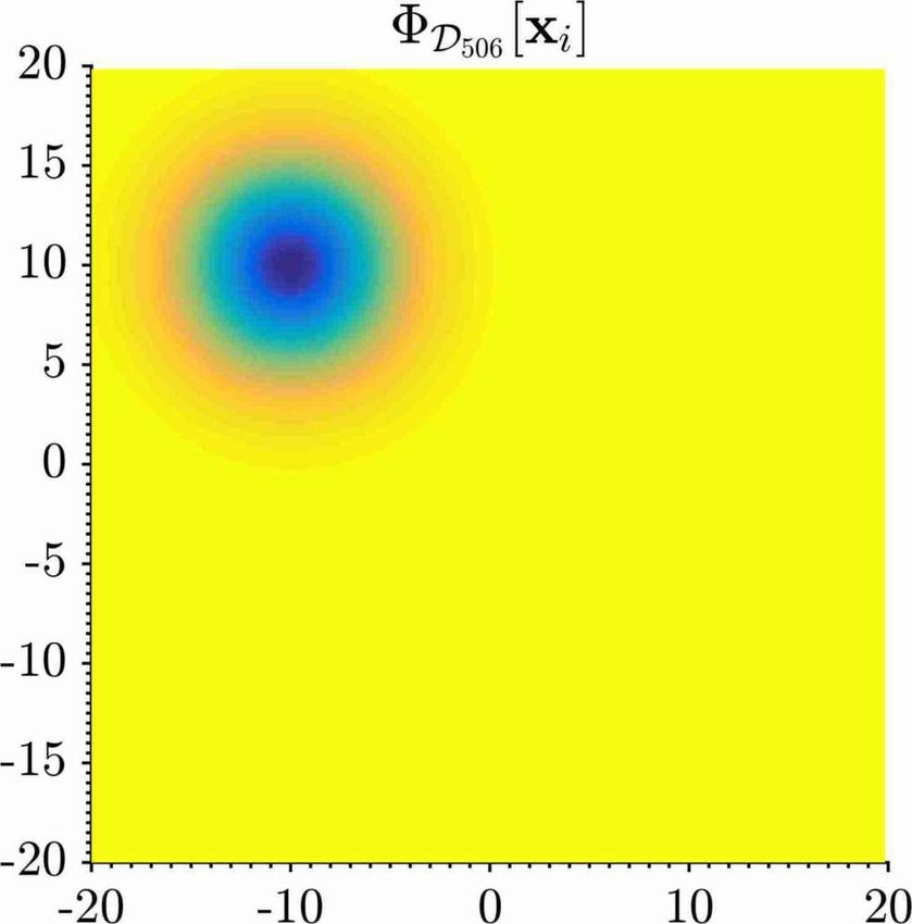
6                                              M. A. Mendez et al
product of two column vectors a, b, and † represents the Hermitian transpose. Similarly,
assuming that the vector ψr [k] ∈ Cnt ×1 collects nt samples of the function ψr (t), defined
in a time domain t ∈ [0, T ], the averaged energy content in the time domain reads:

                        Z                               nt
                    1                                1 X                  1            1
    ||ψr (x)||2 =               ψr (t)ψ r (t) dT ≈         ψr [k]ψ r [k] = hψr , ψr i = ψr† , ψr .   (3.4)
                    T   T                            nt                   nt           nt
                                                       k=1

   Eq.s (3.3) and (3.4) are numerical approximations of the continuous inner products
using the right endpoint rule, and are valuable only if both the spatial and the temporal
discretizations are Cartesian. More advanced quadrature methods or non-uniform dis-
cretization requires the definition of a weighted inner product (Volkwein 2013; Cordier
& Bergmann 2013; Gordeyev & Thomas 2000). To simplify the following derivations, we
nevertheless keep the Euclidean inner products and its simple Cartesian structure.
   From eqs. (3.3)-(3.4), it is clear that the normalization ||φr ||2 = ||ψr ||2 = 1, at a discrete
level, implies that the amplitudes σr in (3.2) must be normalized by ns nt to produce grid-
independent estimations of the energy content of each mode. Before discussing the notion
of energy content, it is useful to arrange the discrete spatial and the temporal structures
into matrices Φ = [φ1 [i] . . . φnt [i]] ∈ Cns ×nt and Ψ = [ψ1 [k] . . . ψnt [k]] ∈ Cnt ×nt . Any
decomposition of the form of Eq.(3.2) becomes a matrix factorization

                                                nt
                                                X
                                          D=          σr φr ψrT = Φ Σ Ψ T ,                          (3.5)
                                                r=1

where Σ = diag[σ1 , σ2 . . . σnt ] is the diagonal matrix containing the energy contribution
of each mode, and the superscript T denotes matrix transposition. Besides allowing for
a compact representation of any decomposition, (3.5) allows for visualizing the operation
as a projection of the dataset onto a spatial basis Φ and a temporal basis Ψ ; the first is
a base for the columns of D; the second is a base for its rows.
   It is worth observing that since Σ is diagonal, defining either Φ or Ψ unequivocally
identifies the other. In this work we focus on projections in the time (row) domain
of the dataset: (3.5) is univocally determined by the choise of Ψ . Moreover, we focus
on orthonormal temporal decompositions, that is Ψ † Ψ = Ψ T Ψ = I, with I the identity
matrix. Computing the spatial structures Φ from (3.5) requires then a right multiplication
by Ψ and a normalization:

                                      Φ = DΨ Σ −1       with    σi = ||D ψr ||2                      (3.6)
                            2
being || • ||2 the L norm. Observe that the orthonormality of Ψ does not imply the
orthonormality of Φ, while if neither of these is orthonormal, computing one from the
other requires a more expensive (and suboptimal) inversion.
   Among the infinite possible orthonormal bases Ψ , we focus on the three most popular
ones: the POD, the DFT and the DMD. The matrix form of these are discussed in the
following subsections. For each of these, the subscripts P, F and D are used to distinguish
the decompositions.
   Before proceeding with their formulation, it is worth commenting on two critical
aspects of any decompositions: 1) the treatment of the time (column-wise) average 2) the
link between the modal contributions σr and the total energy content in D. Concerning
the first point, one can see from (3.2) and (3.5) that the removal of the mean before the
decomposition is equivalent to: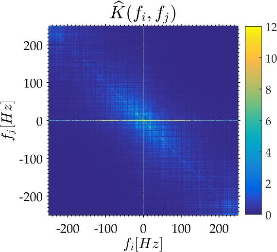
Multi-Scale Proper Orthogonal Decomposition of Complex Fluid Flows                     7

                                                            t          n −1
                              1                            X
              D [i, k] = dµ √ 1T + D̆ [i, k] = σµ φµ 1T +      σ̆r φ̆r [i] ψ̆r [k]    (3.7)
                              nt                           r=1
               Pnt
where dµ [i] =    k=1 dk [i]/nt is the average column of the dataset, with energy content
                                                                             √
σµ = ||dµ || and a constant (and normalized) time evolution of 1/ nt . The D̆ [i, k]
is the zero-mean shifted dataset and the last summation is its modal decomposition
(distinguished by an accent ˘ •). The mean removal reduces the rank of the original matrix,
for which only nt −1 modes remain, and implies that one of the temporal basis is a vector
of constants. All the other –being orthonormal to it– must also have zero mean. This is
naturally the case for the DFT, but not for the POD or the DMD.
   Concerning the second point, the energy content of the dataset can be defined via
different matrix norms. Using the most classical Frobenius norm yields

                                                                       nt
                                                                       X
                                             †              †
                             ||D||2F = Tr(D
                                          | {zD}) = Tr(DD
                                                       | {z }) =              λr             (3.8)
                                              K               C        r=1

where Tr indicates the trace of the matrices K = D† D ∈ Rnt ×nt and C = DD† ∈
Rns ×ns . These are the finite dimensional estimators of the two-point temporal and spatial
correlation tensors (Holmes et al. 2012; Cordier & Bergmann 2013) respectively, using
the inner products in (3.3)-(3.4). These symmetric positive definite matrices share the
same non zero min(ns , nt ) = nt eigenvalues λr . Introducing (3.5) in (3.8) gives two ways
of measuring the total energy from the contribution of each mode:

                                                                               nt
                                                                               X
                                         †        †                     †
                   ||D||2F   = Tr(Ψ
                                  | Σ Φ {zΦ Σ Ψ }) = Tr(Φ
                                                        | Σ{z Φ}) =
                                                                   2
                                                                                     λr .    (3.9)
                                          K                       C            r=1

   It is therefore evident that it is not possible to compute the total energy of the data
by solely using the energy contributions of the modes unless the spatial structures are
also orthonormal (Φ† Φ = I). If this is not the case, neither of the two factorizations of
K and C in (3.9) is an eigenvalue decomposition, and thus the link between σr and λr
involves also the spatial basis.

            3.1. Matrix form of the Proper Orthogonal Decomposition (POD)
  The POD temporal structures ΨP are the orthonormal eigenvectors of the temporal
correlation matrix K = D† D. If D is real, as in most applications, these are real vectors:

                                                      nt
                                                      X
                               K = ΨP ΛP ΨPT =                       T
                                                            λPr ψPr ψP r
                                                                         .                  (3.10)
                                                      r=1

   Introducing this definition in (3.9) is particularly revealing. This choice for the temporal
structure makes the spatial structures also real and orthonormal, that is ΦTP ΦP = I, and
thus eigenvectors of the spatial correlation matrix C = D† D:

                                                      nt
                                                      X
                               C = ΦP ΛP ΦTP =              λPr φPr φTPr .                  (3.11)
                                                      r=1
                                                                         √
  Furthermore, the energy contribution of each mode becomes σPr = λr : the energy
content of the entire dataset can be inferred from the contributions of all the modes Σp .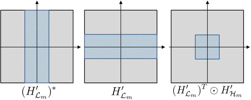
8 M. A. Mendez et al
The original formulation of the POD from Lumley (1967, 1970) computes the spatial
structures ΦP from the eigendecomposition in (3.11); the BOD formulation from Aubry
(1991) computes the temporal structures (referred to as BOD modes) ΨP from the
eigendecomposition in (3.10). The ‘snapshot’ POD from Sirovinch (1987, 1989, 1991)
computes both ΦP and ΨP by first solving (3.10) (computationally less demanding, since
nt
ns ) and then projecting the data using (3.6).
For the choice of inner products in (3.3)-(3.4), (3.5) reduces to the well-known Singular
Value Decomposition (SVD), denoted as D = ΦP ΣP ΨPT . The optimality of the decom-
position is therefore guaranteed by the Eckart-Young-Mirsky theorem, which states that
the approximation of a matrix D constructed by truncating the SVD to rc terms, is the
best rank rc approximation, in that it minimizes the norm of the error
rc
X
T
Err(rc ) = D − σPr φPr ψPr = σPrc +1 . (3.12)
r=1 2
Therefore, each of the coefficients σP represent also the L2 error produced by an
approximation truncated to the previous mode, and the error decay Err(rc ) → 0 as
rc → nt is the strongest possible.
It is in the discussion of energy optimality that one should evaluate the impact of the
mean removal before computing the POD from (3.7). The POD is equipped with a vector
√
of constant 1/ nt as one of its temporal basis only if such a vector is an eigenvector of
K. It is easy to see that this occurs only if:
nt
X
K1 = σ 2 1 ⇐⇒ K[i, j] = σ 2 ∀j ∈ [1, nt ] (3.13)
i=1
that is the sum over any row of K is equal to the corresponding eigenvalue σ 2 . This occurs
for a stationary process, for which the temporal correlation matrix becomes Toepliz
circulant. For a non-stationary process, far from satisfying (3.13), the mean removal
imposes an additional constraint that alters the optimality guaranteed by (3.12).
Finally, it is worth highlighting that the concept of optimality is tightly linked to
that of decomposition uniqueness: in case of repeated singular values, which occurs when
different coherent phenomena have a similar energy content (as shown in §4), there exist
infinite possible choices of singular vectors ΦP and ΨP . This is a significant limitation of
the POD, which in these conditions produces spectral mixing between different modes.
3.2. Matrix form of the Discrete Fourier Transform (DFT)
The DFT temporal structures ΨF are defined a priori, regardless of the dataset at
hand, as column of the well known Fourier Matrix
1 1 1 ... 1
1 1 w w2 ... w(nt −1)
ΨF = √ .. .. .. (3.14)
..
nt .
. . .
2
1 wnt −1 w2(nt −1) . . . w(nt −1)
√
where w = exp 2πj/nt , with j = −1. Each temporal structure is thus a complex
exponential ψr [k] = exp 2πjfr (k − 1)/nt with real frequency fr = (r − 1)∆f , with
∆f = fs /(nt ∆t) the frequency resolution and fs the sampling frequency.
Besides being orthonormal, this Vandermonde matrix is also symmetric, that is ΨFT =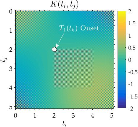
Multi-Scale Proper Orthogonal Decomposition of Complex Fluid Flows 9
ΨF and ΨF−1 = Ψ F . The resulting spatial structures ΦF = DΨ F ΣF −1
from (3.6) are com-
plex and generally not orthogonal. Finally, since the DFT satisfies (3.7) by construction,
the zero-mean shifting has no impact on the decomposition.
3.3. Matrix form of the Dynamic Mode Decomposition (DMD)
The DMD temporal structures ΨD are computed under the assumption that a linear
dynamical system can well approximate the dataset. It is thus assumed that a propagator
matrix P ∈ Rns ×ns maps each column of the data matrix D onto the following one via
simple matrix multiplication
dk = P dk−1 = P k−1 d1 . (3.15)
As each time step k involves the k − 1 power of P acting on the initial data d1 , the
evolution of such linear system depends on the eigendecomposition P = SΛS −1 of the
propagator, since P k−1 = S Λk−1 S −1 :
ns
X
dk [i] = S Λk−1 S −1 d1 [i] = S Λk−1 a0 = a0 [r]sr [i]λk−1
r . (3.16)
r=1
The columns of the eigenvector matrix S = [s1 , s2 , . . . sns ] represent the spatial basis of
such evolution. Observe that the possible decay/growth of each mode makes the notion
of mode ‘amplitude’ particularly cumbersome in the DMD. Instead, the vector a0 =
S −1 d1 is the projection of the initial data d1 onto the eigenvectors of the propagator.
To arrange (3.16) into the factorization of (3.5), one should first arrange the vector of
initial coefficients a0 into a diagonal matrix A0 = diag(a0 ) and then build the temporal
basis from the powers of the eigenvalues. The factorization becomes
λ21 λn1 t
1 λ1 ...
1 λ2 λ22 ... λn2 t
D = S A0 Z T with ZT = . . (3.17)
.. .. ..
.. . . .
1 λns λ2ns ... λnnts
The temporal basis of the DMD is thus finally obtained as ψDm = Zm /||Zm ]||, that is
normalizing Z over each column, and the decomposition completed by (3.6). In this final
step, it is important to observe that the possible exponential decay or growth can make
T
the temporal basis not orthogonal. Therefore, since generally ΨD Ψ D 6= 1, the complex
T +
conjugate of the temporal basis in (3.6) should be replaced by the pseudo-inverse (ΨD ) .
2
To compute a DMD, one needs to calculate the eigenvalues of the best (in a L sense)
propagator describing the dataset. Since the size of this matrix is usually prohibitively
large (ns × ns), this computation must be performed without computing P .
Two classical algorithms have been developed for at the scope, both constructed by
writing (3.15) in a matrix form: given D1 = [d1 , d2 , . . . dnt −1 ] and D2 = [d2 , d3 , . . . dnt ]
two shifted portions containing nt −1 realizations, the propagator is the matrix such that
D2 ≈ [P d1 , P d2 , . . . P dnt −1 ] = P D1 . (3.18)
The first DMD algorithm considered, herein denoted as cDMD, reproduces the action
of the propagator P with a much smaller matrix C ∈ R(nt −1)×(nt −1) acting on the right
side (Rowley et al. 2009). This matrix is the Companion matrix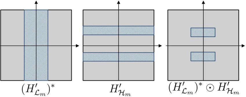
10 M. A. Mendez et al
0 0 ... 0 c1
1 0 0 c2
..
C=
0 1 0 . .
(3.19)
. .. ..
..
. .
0 0 ... 1 cnt −1
The ones in the sub-diagonals shift the columns of D1 to obtain those of D2 ; the last
column contains the set of coefficients c = [c1 , c2 . . . , cnt −1 ]T that approximates the last
temporal realization dnt as a linear combination of the previous:
t −1
nX
d nt ≈ ck dk = D1 c . (3.20)
k=1
These two links between D2 and D1 lead to the equivalence
D2 ≈ D1 C ⇐⇒ P D1 ≈ D1 C , (3.21)
and an eigenvalue λ of the Companion matrix, with eigenvector v, such that Cv = λv,
is also an eigenvalue of P with eigenvector D v. The least square minimization therefore
consists in computing the set of coefficients that minimizes the error ||dnt − D1 c ||.
The solution of this minimization, using a QR factorization D1 = Q R, reads c =
R−1 QT dnt . After using this solution to assemble the matrix C, its diagonalization yields
the eigenvalues required for the definition of the DMD temporal basis ΨD .
This algorithm is an adaptation of the Arnoldi algorithm, a popular power iteration
method (also known as Krylov methods) for computing the eigenvalues of a matrix
(Strang 2007). Its main limitation is the poor conditioning of the matrix C, combined to
its extreme sensitivity on the choice of the first and last data realization and a usually
non-unique solution in the calculation of the coefficients vector c.
The second DMD algorithm considered, herein denoted as sDMD, avoids the calcu-
lation of the Companion matrix and projects the problem onto a space of much lower
dimension (Schmid 2011), in which hopefully only a few eigenvectors are relevant. This
is the space spanned by the first rc dominant POD modes of the dataset.
This propagator is therefore defined as S = Φ̃TP P Φ̃P ∈ Rrc ×rc , where the tilde denotes
an approximation Φ̃P = [φP1 , . . . φPrc ]. Writing the full size propagator as P = D2 D1+
−1 T
from (3.18), with D1+ = Ψ̃P Σ̃P Φ̃P the pseudo-inverse of D1 , gives
−1
S = Φ̃TP P Φ̃P = Φ̃TP D2 Ψ̃P Σ̃P . (3.22)
Observe that (3.22) is a similarity transform, and thus S and P share the same
eigenvalues, only if Φ̃P is a square ns × ns matrix (that is the full POD basis plus
its ns − nt orthogonal complements are taken into account so that Φ̃P Φ̃TP = I). That is
never the case, and one heuristically hopes that at least the first rc eigenvalues of P are
available in S, which implies that Φ̃P Φ̃TP ≈ I.
Although numerically more robust, this POD-based projection can make the decom-
position ill-posed, as discussed with the illustrative test case in §5. This occurs when the
POD basis captures the energy content of the dataset within a few modes, each of which
possibly having several essential frequencies. In this condition, the projected propagator
in (3.22) acts on a space which is too small to allow for a sufficient number of frequencies,
and the DMD decomposition diverges exponentially fast.Multi-Scale Proper Orthogonal Decomposition of Complex Fluid Flows 11
Finally, concerning the mean-shifted form in (3.7), one should notice that the DMD
√
can provide the constant vector 1/ nt as basis element only if λ = 1 is an eigenvalue of
the propagator (C for the cDMD, S for the sDMD). While there is no simple relation to
know when this is the case for S, the characteristic polynomial of C yields:
t −1
nX t −1
nX
if λ=1
p(λ, c) = λnt −1 − ck λk = 0 −−−−→ ck = 1 . (3.23)
k=1 k=1
This condition is not generally imposed to the minimization (3.20), so the DMD basis
might not necessarily have a mode to represent the mean of the dataset. On the other
hand, removing the mean from the dataset results in a complete definition of (3.20), that
is c = [−1, −1, · · · − 1], since the last data realization must cancel the summation. In this
case, as elegantly shown by Chen et al. (2012), the solution of (3.23) are the nt − 1 roots
of unity, and the DMD becomes the DFT.
4. The Multiscale Proper Orthogonal Decomposition (mPOD)
The temporal basis ΨM for the Multiscale Proper Orthogonal Decomposition (mPOD)
proposed in this work is computed by setting frequency constraints to the classical POD.
The algorithm consists of three major steps. First, the temporal correlation matrix
K = D† D is split into the contributions of different scales via Multi-Resolution Analysis
(MRA). This can be performed via 2D Wavelet Transform or more generally via an
appropriate filter bank that is preserves the symmetry of the correlation matrix. Second,
each of these contributions is diagonalized as in the classical POD, to obtain the
orthonormal basis corresponding to each scale. Third, the bases of each scale are merged
into the final temporal basis ΨM , and the decomposition is completed via (3.6).
The theoretical foundation of the algorithm is described in §4.1 and §4.2. In particular,
§4.1 investigates the link between the frequency content in the dataset and that in the
correlation matrix and its eigenvectors. Sec.§4.2 introduces the generalized MRA of K
via filter banks, discussing its impact on the eigenvectors of different scales and the
necessary criteria to keep these mutually orthogonal and free of frequency overlapping.
Finally, section §4.3 presents the proposed mPOD algorithm.
4.1. Mode Spectra and Correlation Spectra
The Multi-Resolution Analysis (MRA) is introduced in §4.2 in the frequency domain,
that is along the 2D Fourier transform of the correlation matrix. It is thus interesting
to analyze the standard POD in the frequency domain. At the scope, we denote as A b
the Discrete Fourier Transform (DFT) of a matrix A, whether this is done along its
rows, columns, or both. Using (3.14), it is easy to see that the DFT of a column vector
is obtained via left multiplication by Ψ F , while the DFT of a row vector is a right
multiplication by Ψ F .
The three Fourier pairs to be linked in this section are related to the time evolution of
the data (D, row-wise), the temporal structures of the POD modes (ΨP , column-wise)
and the temporal correlation matrix (K, over both columns and rows):
b = D Ψ F ⇐⇒ D = D
D b ΨF (4.1a)
ΨbP = Ψ F ΨP ⇐⇒ ΨP = ΨF ΨbP (4.1b)
b = Ψ F K Ψ F ⇐⇒ ΨF K
K b ΨF . (4.1c)12 M. A. Mendez et al
A first link between the DFT of the dataset (4.1a) and that of the POD modes (4.1b)
is identified by the cross-spectral density matrix, defined and linked to the temporal
correlation matrix as follows:
b† D
b = ΨF D† D Ψ F = ΨF K Ψ F ⇐⇒ K = Ψ F KF ΨF .
KF = D (4.2)
This matrix is obtained from the temporal correlation matrix K via a similarity
transform (since ΨF Ψ F = I), and therefore share the same eigenvalues. To link its
eigenvectors to the POD temporal structures, it is important to observe that all the
transformed quantities in 4.1b-4.1c are real, and their Fourier transforms are Hermitian
symmetric, that is have even real part and odd imaginary part.
In matrix notation this can be introduced via a permutation matrix Pπ , which flips
the spectra along the zero frequency (first column of ΨF ). It is worth noticing that this
permutation matrix can be obtained by applying the DFT operator twice:
1 0 ... 0 0
0 0 0 1
..
Pπ = ΨF ΨF = Ψ F Ψ F 0 0
= 1 . . (4.3)
. . ..
.. .. . .. .
0 1 0 ... 0
Observing that the Hermitian symmetry of a complex vector a can be written as Pπ a
leads to the following properties of the first two Fourier pairs in (4.1a)-(4.1b):
Ψbp = Pπ Ψbp ⇐⇒ Ψbp = Pπ Ψbp ⇐⇒ ΨF ΨP = Pπ Ψbp (4.4a)
D b Pπ ⇐⇒ D
b =D b Pπ ⇐⇒ D ΨF = D
b =D b Pπ (4.4b)
Introducing the eigenvalue decomposition of K in (4.2) and using (4.4a) yields
2 †
2 † 2 †
KF = ΨF ΨP ΣP ΨP Ψ F = ΨF ΨP ΣP ΨF ΨP = Pπ ΨbP ΣP Pπ ΨbP . (4.5)
This shows that the eigenvectors of KF are the permuted spectra of the POD modes.
While the similarity argument is essential in any spectral formulation of the POD
(Glauser et al. 1987; Gordeyev & Thomas 2000; Citriniti & George 2000; Gudmundsson
& Colonius 2011; Sieber et al. 2017; Towne et al. 2018), (4.5) shows that care must be
taken with the conjugation (or the flipping of) the eigenvectors before the inverse DFT,
if one seeks to compute POD modes from the cross-spectral density matrix in (4.2).
The DFT of the correlation matrix K in (4.1c), on the other hand, is not obtained via
b 6= K
similarity transform and is not self-adjoint (K b † ). Hence, since it does not share the
same eigenvalues of K and KF , its diagonalization is of no interest for the purpose of
this work. However, because of its relevance on the filtering process, it is important to
highlight – by introducing (4.2) into (4.1c)– its link to KF :
b = Ψ F Ψ F KF ΨF Ψ F = Ψ F Ψ F KF = Pπ KF .
K (4.6)
4.2. Decomposing Data and Decomposing Correlations
It is now of interest to understand how a temporal filtering of the dataset influences
the frequency content of the POD modes. In particular, we are interested not in justMulti-Scale Proper Orthogonal Decomposition of Complex Fluid Flows 13
Figure 1: Multi-Resolution Analysis (MRA) of the time signal dp [k] using a filter bank
illustrated along its frequency spectrum dbp [n]. The MRA splits the spectra into of a large
scale (low frequency portion) identified by the transfer function HL1 , m ∈ [2, . . . M −
1] intermediate scales identified by the transfer functions HHm , and a fine scale (high
frequency portion) identified by the transfer functions HHM . Only the positive portion
of the spectra is shown, the negative one being mirrored along the ordinates.
one filter, but an array of filters, constructed to isolate different portions of the dataset
spectra. To illustrate the idea, let us consider the Fourier transform dbp = dp Ψ F of the
temporal evolution of the data in a specific point, that is dp [k] = D[ip , k].
We seek to split the spectra dbp into the contributions of M different scales, each
retaining a portion with negligible overlapping as pictorially illustrated in Figure 1.
c c
The frequency bandwidths ∆fm = fm+1 − fm are not necessarily of equal length,
but controlled by a frequency splitting vector FV = [f1c , f2c , . . . fM
c
−1 ], bounded by the
minimum (fn = 0) and the maximum (|fn | = fs /2) discrete frequencies possible.
This splitting requires the definition of a filter bank (Vaidyanathanm 1992; Strang &
Nguyen 1996; Shukla & Tiwari 2013), consisting of a low-pass filter with cut off f1c , a
c
high-pass filter with cut off fM , and M − 2 band-pass filters between these. The modulus
of the transfer functions of these filters is shown in Figure 1 with a continuous line.
Following the lossless formulation common in multi-resolution analysis, these filters are
constructed from the set of m ∈ [1, . . . M ] low pass filters with transfer function HLm ,
shown in figure 1 with dashed line. The transfer functions of the band-pass filters HHm
are computed as complementary differences HHm = HLm+1 − HLm , the finest one being
HHM = 1 − HLM . By construction, the lossless decomposition of the signal implies that
HL1 + HH1 · · · + HHM = 1. The design of the set of the low-pass filters defining the filter
bank is presented in Appendix A; in what follows we focus on the algebra of the filtering
process and the theoretical foundation of the proposed mPOD.
Considering the filtering in the frequency domain, this operation is performed via
simple multiplication (entry by entry), which in matrix notation corresponds to the
Hadamard product . Moreover, since each of these filters is applied in the entire spatial14 M. A. Mendez et al
domain (along each row of D), one should copy the transfer functions HLm or HHm (row
vectors ∈ C1×nt ) to obtain ns × nt matrices having all the rows equal to HLm or HHm .
This bi-dimensional extension of the 1D transfer function is here indicated with an apex,
0
so that Hm denotes the general transfer function (whether low pass or band pass). The
contribution of a scale m from figure 1 in each of the spatial points (that is the filtered
portion of the dataset) is
D
bm
hz }| i{
0
Dm = D ΨF Hm ΨF . (4.7)
| {z }
D
b
The first multiplication is the DFT along the time domain (D), b the result of the
Hadamard multiplication in the square bracket is the filtered spectra of the data (D
b m,
the frequency contribution of the given scale) and the last right multiplication is the
†
inverse DFT from (4.1a). Using (4.7), the correlation matrix Km = Dm Dm from each
scale contribution reads
h † i h i
0 0 b † D) 0 † 0
Km = Ψ F Db Hm D
b Hm ΨF = Ψ F D b (Hm ) Hm ΨF , (4.8)
where the associative and commutative properties of the Hadamard product are used to
move the transfer functions. Recognizing the cross-spectral density matrix KF in (4.5)
0 † 0
and writing the 2D transfer function as Hm = (Hm ) Hm yields
h i h i
Km = Ψ F KF H m ΨF = ΨF Kb Hm ΨF , (4.9)
| {z } | {z }
KF m K
bm
having introduced (4.6) in the last step.
This important result lays the foundation of the mPOD. First, the expression on the left
of (4.9) is a similarity transform: the filtered cross-spectral density KF m = KF Hm
†
shares the same eigenvalues of the correlation of filtered data Km = Dm Dm . Second,
introducing the eigenvalue decomposition of Km as in (4.5), shows that –up to a
permutation– the eigenvectors of KF are the DFT of the POD modes of the filtered
problem:
2 † 2 †
KF m = ΨF Km Ψ F = ΨF ΨPm ΣPm ΨPm Ψ F = Pπ ΨbPm ΣPm Pπ ΨbPm , (4.10)
having introduced (4.4a) in the last step. The impact of the filter on the POD modes
becomes therefore evident from the entries of KF m and KF along their diagonals, which
are summations of nonnegative real numbers. From (4.10) and (4.4a), it is
nt
X †
2
KF [i, j] Hm [i, j] = KF m [i, j] = σPm r ψ Pm r [i] ψ Pm r [j] .
b b (4.11)
r=1
If the filter at a given scale m removes one of the entries along the diagonal of KF
(Hm [i, i] = 0), the associated frequency ψbPm r [i] cannot be present in any of the r POD
modes of the filtered data: the POD operating at this scale is constrained within the
frequencies allowed by the transfer function.
Moreover, while the expression on the right side of (4.9) is not a similarity transform, it
shows that the correlation matrix associated to the filtered data Km can be computed byMulti-Scale Proper Orthogonal Decomposition of Complex Fluid Flows 15
Approximation (hLm ⊗ hLm ) Vertical Detail (hLm ⊗ hHm )
Diagonal Detail (hHm ⊗ hHm ) Horizontal Detail (hHm ⊗ hVm )
Figure 2: Modulus of the four possible 2D transfer functions Hm that can be obtained
by combining the low-pass (HLm ) and the high-pass (HHm ) filters associated to a given
scale Km , following the multi-scale architecture in figure 1. The areas where the transfer
function is ∼ 1 and ∼ 0 are indicated with blue dashed lines and full gray respectively.
In 2D wavelet terminology, the contributions identified by these four transfer functions
are the approximation and the diagonal, horizontal and vertical details.
a simple 2D filtering of the original correlation matrix, saving considerable computational
time with respect to ns filters along the rows of D. Eq.(4.9) shows that the MRA of the
dataset can be carried out via 2D MRA of the temporal correlation matrix.
The four possible structures for the 2D transfer functions Hm that arise from a
combination of the 1D kernels in the time domain are illustrated graphically in Figure 2.
For a given scale, composed of a low frequency and a high frequency Dm = DLm + DHm ,
these correspond to the contributions of four temporal correlation matrices:
† † † † †
Km = Dm Dm = DL m
DLm + DH m
DHm + DL m
DHm + DH m
DLm
h i (4.12)
= ΨF K b H b H b H b H
Lm + K Hm + K LHm + K HLm ΨF
† †
The ‘pure’ terms DL m
DLm and DH m
DHm are those that can be obtained by first
filtering the data (4.7) and then computing the related correlations; the mixed terms can
only be revealed by a MRA of the full correlation matrix Km .
It is interesting to observe that the filter bank architecture described in this section
is a generalized version of the MRA via Discrete (Dyadic) Wavelet Transform (DWT)
proposed in previous works (Mendez et al. 2018a,b). In the 2D wavelet terminology, the
four terms in (4.12), with spectral band-pass region illustrated in figure 2, correspond to
the approximation and the diagonal, horizontal and vertical details of each scale.
† †
Particular emphasis should be given to the ‘pure’ terms DL m
DLm and DH m
DHm
corresponding to the approximation and the diagonal details. These contributions have no
frequency overlapping and their eigenspaces are orthogonal complements by construction:
their set of eigenvectors can be used to assemble an orthogonal basis as illustrated in §4.3.
† †
The mixed terms DL m
DHm and DH m
DLm , on the other hand, generates eigenspaces that
can potentially overlap with those of the ‘pure’ contributions.
To understand when this occurs, one should first notice that under the assumption of16 M. A. Mendez et al
perfect frequency detection (infinitesimal frequency resolution), their contribution should
be null. Every harmonic phenomenon, evolving at a frequency fA , can only correlate with
itself if the observation time is sufficiently large to avoid the windowing problem (spectral
leakage, Harris (1978)), or if the considered frequency is among those available in the DFT
spectra. For an infinitely fine resolution, such phenomenon produces a Dirac pulse along
the diagonal and the anti-diagonal of K b m (and thus K) b and it is visible only in the
corresponding band-pass portion (diagonal detail, second row in figure 2).
However, the finite frequency resolution results in several secondary peaks, which in
a 2D spectra appear as cross-like patterns centered at the main peak (see Figures 8 or
19). Depending on how narrow the bands of the frequency splitting vector FV are, these
secondary peaks can extend outside the frequency band of the pure terms, and appear
in both the horizontal and the vertical details. In such a case, removing the mixed terms
from (4.12) compromises the perfect reconstruction of the temporal correlation matrix
and, if only harmonic bases are allowed as in the DFT, the well-known Gibbs phenomenon
(see Folland (2009)) is produced.
The freedom in the choice among all the possible discrete frequencies in KF m for each of
the modes is what allows the POD for avoiding these problems. The mPOD reduces such
freedom, to an extent that depends on how narrow the bandpass of each scale is allowed
† †
to be. However, while neglecting the mixed terms DLm DHm and DHm DLm prevents
the perfect reconstruction of the correlation matrix, it does not prevent the lossless
reconstruction of the dataset since the final assembled temporal basis is complete. At
the limit FV → fn , that is when each scale is allowed to act only on a single frequency,
the mPOD preserves just the diagonal and the antidiagonal of K b and the eigenspace
of each contribution K b m consists of a single harmonic. The loss of information in the
approximation of the correlation matrix is the maximum possible, and the mPOD reduces
to the DFT.
4.3. The mPOD algorithm
The steps of the proposed mPOD algorithm are recalled in the Algorithm 1. As for
any data-driven decomposition, the first step consists in assembling the data matrix as
in (3.1). The second step consisting in computing the temporal correlation matrix K and
its Fourier transform K b from (4.1c).
From the analysis of the frequency content in the correlation spectra K, b the third
step consists in defining the frequency splitting vector FV and in constructing the set
of associated transfer functions. This vector can be defined a priori if the user has prior
knowledge on the investigated data or can be inferred automatically by centering the
band-pass windows of each scale on the dominant peaks in the diagonal of K b and
splitting the band-pass regions accordingly. In this step, only the ‘pure’ (approximation
and diagonal detail) terms of the 2D transfer functions are constructed, that is HL1 =
(HL0 1 )† HL0 1 and HHm = (HH 0
m
) † HH 0
m
. Disregarding the mixed terms (horizontal
and vertical details) in each scale, the correlation matrix is approximated as:
h i M
X h i M
X −1
K ≈ ΨF Kb H L1 Ψ F + ΨF Kb HHm Ψ F ≈ KL1 + KHm . (4.13)
m=1 m=1
Each of these contributions is a symmetric, real and positive definite matrix, equipped
with its orthonormal eigenspace, computed in the fourth stepMulti-Scale Proper Orthogonal Decomposition of Complex Fluid Flows 17
Input: Set of nt snapshots of a dataset D(xi , tk ) on a Cartesian grid xi ∈ Rnx ×ny
1: Reshape snapshots into column vectors dk [i] ∈ Rns ×1 and assemble D[i, k] in (3.1)
2: Compute time correlation matrix K = D† D and K b = Ψ F K Ψ F in (4.1c)
3: Prepare the filter bank HL1 , . . . HHM and split K into M contributions via (4.13)
2 T
4: Diagonalize each ‘pure’ term Km = Ψm Σm Ψm as in (4.14)
0
5: Sort the contribution of all the scales into ΨM as in (4.15)
6: Enforce orthogonality via QR Factorization, ΨM 0
= ΨM R → ΨM = ΨM 0
R−1
−1
7: Compute the spatial basis ΦM = D ΨM ΣM from (3.6) and sort the results in
descending order of energy contribution.
Output: Spatial ΦM and temporal ΨM structures with corresponding amplitudes ΣM of
the nt mPOD modes.
Algorithm 1: Multi-scale Proper Orthogonal Decomposition of a dataset D ∈ Rns ×nt .
M
X −1
K≈ ΨL1 ΣL2 1 ΨLT1 + 2
ΨHm ΣH ΨT .
m Hm
(4.14)
m=1
As demonstrated in §4.2, if the frequency-overlapping is identically null, the eigenspaces
of these pure terms are orthogonal complements, and therefore there are at most nt non-
zero eigenvalues among all the scales. This is a major difference between the mPOD and
other multi-scale methods such as Continuous Wavelet Transform (CWT), in which the
temporal basis is constructed by shifting and dilating a ‘mother’ function, or the multi-
resolution DMD (mrDMD) proposed by Kutz et al. (2016b), in which the temporal
basis is constructed by performing DMD on different portions of the datasets. These
decompositions potentially produce high redundancy and poor convergence since the
basis is larger than nt . Moreover, each of the basis elements in the mPOD exists over
the entire time domain (although they could be null in an arbitrarily large portion of
it), whiles in CWT or mrDMD produce different bases for different portions of the time
domain, leading to decompositions more complicated than those analyzed in this work.
Because of the limited size of the filter impulse response (see Annex A) of each filter,
the number of non-zero eigenvalues among the scales is in practice usually slightly larger
than nt . Therefore, only the first nt dominant eigenvectors are selected. This is done
in the fifth step, using the eigenvalue matrices ΣL2 1 , ΣH
2
m
to re-arrange the eigenvector
matrices ΨL , ΨHm into one single matrix (temporal basis)
0
ΨM = ΨL1 , ΨH1 , ΨH2 . . . ΨHM . (4.15)
The columns of this matrix are permuted to respect the descending order of the
associated eigenvalues ΣL2 1 , ΣH
2
m
, regardless of their scale of origin.
As demonstrated in §4.2, the temporal matrix (4.15) is orthonormal if a perfect spectral
separation is achieved. This is a major difference between the mPOD and the SPOD by
Sieber et al. (2016), in which the filtering procedure can eventually result in a non-
orthogonal temporal basis, or the mrDMD by Kutz et al. (2016b), in which decaying
modes might produce non-orthogonal bases.
Once again, however, due to the finite size of the transition band of the filters, this is
generally not the case in practice, and a minor loss of orthogonality usually occurs. The
sixth step treats this imperfection, polishing this temporal structure via a reduced QR
0
factorization ΨM = ΨM R. This compensates the losses of orthogonality and removes the18 M. A. Mendez et al
T1 (tk ) T2 (tk ) T3 (tk )
0.1
0.1
0.05
0 0 0
-0.05
-0.1
-0.1
0 1 2 3 4 5 0 1 2 3 4 5 0 1 2 3 4 5
tk tk tk
Figure 3: Spatial (top row) and corresponding temporal (bottom row) structures of
the modes considered in the simplified test case. The amplitude of each contribution
is computed so as to give the energy content. An animation of this test case is available
as supplemental Movie 1.
extra columns so that ΨM = ΨM 0
R−1 ∈ Rnt ×nt . The upper triangular matrix R offers
the user an indication on the quality of the filtering process, being close to the identity
when the spectral overlapping is negligible.
Finally, in the last step the decomposition is completed via the projection and the
normalization in (3.6), as for any orthogonal decomposition.
5. Example I: Illustrative Synthetic Test
5.1. Dataset Description
As a first example, we propose a simple synthetic test case which is already in the de-
composed form of (3.5) and yet capable of severely challenging standard decompositions.
The spatial domain consists of a square Cartesian grid of ns = 256 × 256 points over a
domain xi ∈ [−20, 20] × [−20, 20], while the time domain spans tk ∈ [0, 5.11] with a total
of nt = 256 points with sampling frequency fs = 100. The dataset is composed of the
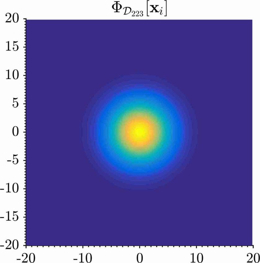
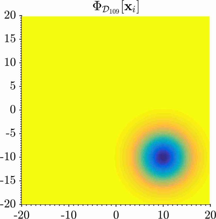
sum of three modes, having spatial and temporal structures as illustrated in Figure 3.
These modes consist of identical Gaussians with standard deviations of σ = 5, located in
x1 = [10, −10], x2 = [−10, 10] and x3 = [0, 0], pulsing as
" #20
(tk − 4)2
T1 (tk ) = A1 sin 2πf1 tk exp (5.1a)
100
π
T2 (tk ) = A2 sin 2πf2 tk − (5.1b)
3
T3 (tk ) = A3 sin 2πf3 tk (tk − 2.55)2 . (5.1c)
The first mode has a smoothed square box modulation, the second has a harmonic with
period longer than the observation time and the third has a parabolic modulation. The
amplitude of each contribution is computed so as to give the same energy (norm) to each
mode, while the three frequencies are f1 = 15, f2 = 0.1 and f3 = 7. The resulting dataset
D[i, k] is a matrix of size 65536 × 256 of rank rk(D) = 3.You can also read