Coloring Concept Detection in Video using Interest Regions - Koen Erik Adriaan van de Sande
←
→
Page content transcription
If your browser does not render page correctly, please read the page content below

Coloring Concept Detection in Video
       using Interest Regions

      Koen Erik Adriaan van de Sande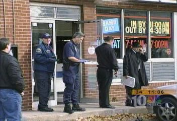
2
Coloring Concept Detection in Video
       using Interest Regions

       Doctoraal Thesis Computer Science
 specialization: Multimedia and Intelligent Systems

         Koen Erik Adriaan van de Sande
                ksande@science.uva.nl

              Under supervision of:
               Prof. Dr. Theo Gevers
                        and
               Dr. Cees G.M. Snoek

                   March 12, 2007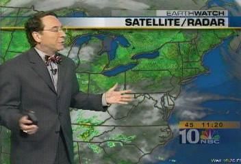
4

Abstract
Video concept detection aims to detect high-level semantic information present in video.
State-of-the-art systems are based on visual features and use machine learning to build
concept detectors from annotated examples. The choice of features and machine learning
algorithms is of great influence on the accuracy of the concept detector. So far, intensity-
based SIFT features based on interest regions have been applied with great success
in image retrieval. Features based on interest regions, also known as local features,
consist of an interest region detector and a region descriptor. In contrast to using
intensity information only, we will extend both interest region detection and region
description with color information in this thesis. We hypothesize that automated concept
detection using interest region features benefits from the addition of color information.
Our experiments, using the Mediamill Challenge benchmark, show that the combination
of intensity features with color features improves significantly over intensity features
alone.

                                             5
6
Contents
1 Introduction                                                                                                                        9

2 Related work                                                                                                                        11
  2.1 Content-Based Image Retrieval       .   .   .   .   .   .   .   .   .   .   .   .   .   .   .   .   .   .   .   .   .   .   .   11
      2.1.1 Datasets . . . . . . . . .    .   .   .   .   .   .   .   .   .   .   .   .   .   .   .   .   .   .   .   .   .   .   .   11
      2.1.2 Image indexing . . . . .      .   .   .   .   .   .   .   .   .   .   .   .   .   .   .   .   .   .   .   .   .   .   .   12
  2.2 Video retrieval . . . . . . . . .   .   .   .   .   .   .   .   .   .   .   .   .   .   .   .   .   .   .   .   .   .   .   .   14
      2.2.1 Datasets . . . . . . . . .    .   .   .   .   .   .   .   .   .   .   .   .   .   .   .   .   .   .   .   .   .   .   .   16
      2.2.2 Video indexing . . . . .      .   .   .   .   .   .   .   .   .   .   .   .   .   .   .   .   .   .   .   .   .   .   .   16
  2.3 Conclusions . . . . . . . . . . .   .   .   .   .   .   .   .   .   .   .   .   .   .   .   .   .   .   .   .   .   .   .   .   18

3 Coloring concept detection using interest regions                                                                                   19
  3.1 Reflection model . . . . . . . . . . . . . . . . . . . .                            .   .   .   .   .   .   .   .   .   .   .   19
      3.1.1 Modelling geometry changes . . . . . . . . . .                                .   .   .   .   .   .   .   .   .   .   .   21
      3.1.2 Modelling illumination color changes . . . . .                                .   .   .   .   .   .   .   .   .   .   .   21
  3.2 Color spaces and invariance . . . . . . . . . . . . . .                             .   .   .   .   .   .   .   .   .   .   .   21
      3.2.1 RGB . . . . . . . . . . . . . . . . . . . . . . .                             .   .   .   .   .   .   .   .   .   .   .   21
      3.2.2 Normalized RGB . . . . . . . . . . . . . . . .                                .   .   .   .   .   .   .   .   .   .   .   23
      3.2.3 HSI . . . . . . . . . . . . . . . . . . . . . . .                             .   .   .   .   .   .   .   .   .   .   .   23
      3.2.4 Opponent color space . . . . . . . . . . . . .                                .   .   .   .   .   .   .   .   .   .   .   24
  3.3 Color constancy . . . . . . . . . . . . . . . . . . . . .                           .   .   .   .   .   .   .   .   .   .   .   25
  3.4 Image derivatives . . . . . . . . . . . . . . . . . . . .                           .   .   .   .   .   .   .   .   .   .   .   25
  3.5 Interest point detectors . . . . . . . . . . . . . . . .                            .   .   .   .   .   .   .   .   .   .   .   27
      3.5.1 Harris corner detector . . . . . . . . . . . . .                              .   .   .   .   .   .   .   .   .   .   .   27
      3.5.2 Scale selection . . . . . . . . . . . . . . . . .                             .   .   .   .   .   .   .   .   .   .   .   28
      3.5.3 Harris-Laplace detector . . . . . . . . . . . .                               .   .   .   .   .   .   .   .   .   .   .   29
      3.5.4 Color boosting . . . . . . . . . . . . . . . . .                              .   .   .   .   .   .   .   .   .   .   .   29
      3.5.5 ColorHarris-Laplace detector . . . . . . . . .                                .   .   .   .   .   .   .   .   .   .   .   30
  3.6 Region descriptors . . . . . . . . . . . . . . . . . . .                            .   .   .   .   .   .   .   .   .   .   .   31
      3.6.1 Color histograms . . . . . . . . . . . . . . . .                              .   .   .   .   .   .   .   .   .   .   .   31
      3.6.2 Transformed color distribution . . . . . . . .                                .   .   .   .   .   .   .   .   .   .   .   32
      3.6.3 Hue histogram . . . . . . . . . . . . . . . . .                               .   .   .   .   .   .   .   .   .   .   .   32
      3.6.4 Color-based moments and moment invariants                                     .   .   .   .   .   .   .   .   .   .   .   33
      3.6.5 SIFT . . . . . . . . . . . . . . . . . . . . . . .                            .   .   .   .   .   .   .   .   .   .   .   33
  3.7 Visual vocabulary . . . . . . . . . . . . . . . . . . .                             .   .   .   .   .   .   .   .   .   .   .   34
      3.7.1 Clustering . . . . . . . . . . . . . . . . . . . .                            .   .   .   .   .   .   .   .   .   .   .   34
      3.7.2 Similarity measures . . . . . . . . . . . . . .                               .   .   .   .   .   .   .   .   .   .   .   35
  3.8 Supervised machine learning . . . . . . . . . . . . . .                             .   .   .   .   .   .   .   .   .   .   .   36

4 Concept detection framework                                                                                                         37

5 Concept detection system                                                                                                            39
  5.1 Feature extraction . . . . . . . . . .          .   .   .   .   .   .   .   .   .   .   .   .   .   .   .   .   .   .   .   .   39
  5.2 Detectors . . . . . . . . . . . . . . .         .   .   .   .   .   .   .   .   .   .   .   .   .   .   .   .   .   .   .   .   40
  5.3 Region descriptors . . . . . . . . . .          .   .   .   .   .   .   .   .   .   .   .   .   .   .   .   .   .   .   .   .   43
      5.3.1 RGB histogram . . . . . . . .             .   .   .   .   .   .   .   .   .   .   .   .   .   .   .   .   .   .   .   .   43
      5.3.2 Transformed RGB histogram                 .   .   .   .   .   .   .   .   .   .   .   .   .   .   .   .   .   .   .   .   44
      5.3.3 Opponent histogram . . . . .              .   .   .   .   .   .   .   .   .   .   .   .   .   .   .   .   .   .   .   .   44
      5.3.4 Hue histogram . . . . . . . .             .   .   .   .   .   .   .   .   .   .   .   .   .   .   .   .   .   .   .   .   44
      5.3.5 Color moments . . . . . . . .             .   .   .   .   .   .   .   .   .   .   .   .   .   .   .   .   .   .   .   .   44
      5.3.6 Spatial color moments . . . .             .   .   .   .   .   .   .   .   .   .   .   .   .   .   .   .   .   .   .   .   45

                                              7
5.3.7 Spatial color moments with normalized RGB                                        .   .   .   .   .   .   .   .   .   .   .   45
         5.3.8 Color moment invariants . . . . . . . . . . . .                                  .   .   .   .   .   .   .   .   .   .   .   45
         5.3.9 Spatial color moment invariants . . . . . . . .                                  .   .   .   .   .   .   .   .   .   .   .   45
         5.3.10 SIFT . . . . . . . . . . . . . . . . . . . . . . .                              .   .   .   .   .   .   .   .   .   .   .   45
   5.4   Clustering . . . . . . . . . . . . . . . . . . . . . . . .                             .   .   .   .   .   .   .   .   .   .   .   45
         5.4.1 K-means clustering . . . . . . . . . . . . . . .                                 .   .   .   .   .   .   .   .   .   .   .   45
         5.4.2 Radius-based clustering . . . . . . . . . . . .                                  .   .   .   .   .   .   .   .   .   .   .   46
         5.4.3 Visual vocabulary . . . . . . . . . . . . . . .                                  .   .   .   .   .   .   .   .   .   .   .   46
         5.4.4 Similarity measures . . . . . . . . . . . . . .                                  .   .   .   .   .   .   .   .   .   .   .   47
   5.5   Concept detector pipeline . . . . . . . . . . . . . . .                                .   .   .   .   .   .   .   .   .   .   .   47
   5.6   Feature fusion . . . . . . . . . . . . . . . . . . . . . .                             .   .   .   .   .   .   .   .   .   .   .   48

6 Experimental setup                                                                                                                        49
  6.1 Experiments . . . . . . . . . . . . . . . . . . . . . . . . . . . . . . . . . .                                                       49
  6.2 Mediamill Challenge . . . . . . . . . . . . . . . . . . . . . . . . . . . . .                                                         49
  6.3 Evaluation criteria . . . . . . . . . . . . . . . . . . . . . . . . . . . . . .                                                       49

7 Results                                                                                                                                   53
  7.1 Machine learning algorithms       .   .   .   .   .   .   .   .   .   .   .   .   .   .   .   .   .   .   .   .   .   .   .   .   .   53
  7.2 Visual vocabulary . . . . .       .   .   .   .   .   .   .   .   .   .   .   .   .   .   .   .   .   .   .   .   .   .   .   .   .   54
  7.3 Global and local features . .     .   .   .   .   .   .   .   .   .   .   .   .   .   .   .   .   .   .   .   .   .   .   .   .   .   55
  7.4 Color constancy . . . . . . .     .   .   .   .   .   .   .   .   .   .   .   .   .   .   .   .   .   .   .   .   .   .   .   .   .   57
  7.5 Feature fusion . . . . . . . .    .   .   .   .   .   .   .   .   .   .   .   .   .   .   .   .   .   .   .   .   .   .   .   .   .   58

8 Conclusions                                                                                                                               61

A TRECVID Participation                                                                                                                     63

                                                    8
1    Introduction
In the digital age we live in, more and more video data becomes available. Television
channels alone create thousands of hours of new video content each day. Due to the sheer
volume of data, it is impossible for humans to get a good overview of the data available.
Retrieving specific video fragments inside a video archive is only possible if one already
knows where to search for or if textual descriptions obtained from speech transcripts or
social tagging are available. Video retrieval can be applied to video collections on the
internet, such as YouTube [53] and Yahoo Video [52], to news video archives, to feature
film archives, etc. Currently, the search capabilities offered by these video collections
are all based on text. The addition of text by humans is very time consuming, error
prone and costly and the quality of automatic speech recognition is poor. Contrary to
the text modality, the visual modality of video is always available.
    Unfortunately the visual interpretation skills of computers are poor when compared
to humans. However, computers are experts in handling large amounts of binary data.
Computers can decode video streams into individual video frames and compute statistics
over them, but there is a big gap between the machine description ‘this frame contains
a lot of green’ and the soccer match that humans see. To associate high level semantic
concepts such as soccer to video data, we need to bridge the semantic gap. The semantic
gap has been defined by Smeulders et al [38] as follows:
    “The semantic gap is the lack of coincidence between the information that machines
can extract from the visual data and the interpretation that the same data have for a
user in a given situation.”
    State-of-the-art systems in both image retrieval [48, 18, 54] and video retrieval [33]
use machine learning to bridge the gap between features extracted from visual data
and semantic concepts. Semantic concepts are high-level labels of the video content.
Systems learn semantic concept detectors from features. The accuracy of the concept
detector depends on the feature used, the machine learning algorithm and the number
of examples. The feature is one of the building blocks of a concept detector and its
choice is very important for performance.
    In concept-based image retrieval, SIFT features [21] based on interest regions are
state-of-the-art [54]. These features consist of an interest region detector and a region
descriptor. However, both components operate on intensity information only: they com-
pletely discard the color information present. The question arises why color information
is neglected. We hypothesize:
    Automated concept detection using interest region features benefits from the addition
of color information.
    Our goal is to extend both interest region detection and interest region description
with color. We evaluate the SIFT region descriptor and color region descriptors. Criteria
for selecting the descriptors include invariance against variations in light intensity, illu-
mination color, view geometry, shadows and shading. If the descriptor used is invariant
to a condition, then the concept can be detected even if the condition changes. We com-
pute the descriptors over either entire video frames or over interest regions. The former
are called global features, while the latter are local features. Depending on the region
over which we compute descriptions, we can achieve invariance against scale changes,
rotation or object position changes. For example, when the position of an object in
the scene changes, the task of learning a concept detector is simplified if the feature
vector remains similar. For local features, we have both an intensity interest region
detector and a color-extended interest region detector. Furthermore, we investigate how
to best aggregate the descriptors of many interest regions into a single feature vector.
Finally, we investigate whether combinations of features provide benefits over individ-
ual features. We perform our large-scale evaluation of visual features using 85 hours of

                                             9
video from the Mediamill Challenge [42], a benchmark for automated semantic concept
detection.
    The organization of this thesis is as follows. In chapter 2, we give an overview of
related work. In chapter 3, we provide the necessary background for our generic concept
detection framework, discussed in chapter 4. In chapter 5, we provide implementation
details of our concept detection system. In chapter 6, we describe our experimental
setup. In chapter 7, we show the results of our system. Finally, in chapter 8, we draw
conclusions and provide directions for future research.

                                          10
2 Related work
In this chapter, we will discuss research related to automatic semantic concept detection.
Concept detection has already been extensively studied in the field of Content-Based
Image Retrieval (CBIR), where concepts are referred to as categories. In section 2.1,
we discuss the datasets and methods used in CBIR. In section 2.2, we compare this to
work in the video retrieval field. Finally, in section 2.3, we conclude with the rationale
for our work on concept detection in video.
2.1 Content-Based Image Retrieval
The field of Content-Based Image Retrieval studies, amongst others, the application of
computer vision in the context of image retrieval. Then, the image retrieval problem
corresponds to the problem of searching for digital images in datasets. Because this
thesis focuses on the detection of concepts, other important issues of CBIR, such as
visualization, image databases, etc. are beyond the scope of this thesis and will not be
discussed here.
Content-Based Image Retrieval systems tend to follow a common scheme. First,
a description of every image in the dataset is computed. A description is a concise
representation of the image contents, typically taking the form of a numeric feature
vector. Second, these descriptions are indexed to speed up the search process. Third,
the description of an unseen image is computed. Unseen images can be assigned to a
category depending on which categories similar descriptions come from.
We perceive the task of assigning a category to an unindexed image as a machine
learning problem: Given a number of feature vectors (descriptions of images) with corre-
sponding class labels (categories), the aim is to learn a classifier function which estimates
the category of unseen feature vectors.
One of the most important properties of image descriptions for robust retrieval is
invariance to changes in imaging conditions. For example, after rotation or scaling of
the object in view, the image of the object should still be retrieved. Moreover, more
complex imaging transformations such as object position and viewpoint changes should
be handled. Other possible changes are photometric changes (light intensity, color of
the light source, etc) and object shape changes. Different degrees of invariance can be
achieved for variations in imaging conditions. However, increased invariance comes at
the cost of reduced discriminability [12]. For example, for an image description which
is invariant for the color of the light source it will be difficult to distinguish between a
room with a white light source and a room with a red light source.
Because we perceive CBIR as a machine learning task, the classification scheme only
applies when annotations for the original dataset are available. Methods which do not
require annotations are unsupervised methods. These methods find clusters of similar
items in a dataset. However, further human interpretation of these clusters is needed,
because they do not assign semantic labels to the images. For example, the Query-
by-Example retrieval method finds items similar to given examples, but these items
need to be judged by a human. In combination with visualization tools, unsupervised
methods are very useful for analysis of the nature of image descriptions. Depending on
the description used, different images will be clustered together.
2.1.1 Datasets
To evaluate results in the CBIR field, many image datasets have been generated. Because
the focus is on concept detection, only datasets are discussed which divide the images
into different concept categories. In table 1 several datasets and their properties are
listed.
11Name # images # concepts Properties
Xerox7 [51] 1,776 7 highly variable pose and background clutter,
large intra-class variability
CalTech6 [8] 4,425 6 background set without concepts available,
same pose within an object class, object
prominently visible near image center
PASCAL dataset [5] 2,239 4 object location annotations available, multi-
ple instances per image allowed
CalTech101 [7] 8,677 101 little or no clutter, objects tend to be cen-
tered and have similar pose
Corel photo stock 16,499 89 high quality images, variable poses, low
(commercial) background clutter
Amsterdam Library 110,250 1000 objects photographed in different poses un-
of Object Images der varying lighting conditions, objects are
(ALOI) [11] centered, black background
Table 1: Concept-based datasets from content-based image retrieval.
The image datasets listed, except the Corel and ALOI, consist of only several thou-
sands of images. Compared to the sizes of real-world image collections, they are relatively
small. In fact, the datasets have been designed to evaluate ‘desired’ invariance proper-
ties of new descriptors. Because of this, some of the datasets impose certain conditions
on the images (objects in similar pose, no background, object is centered, professional
photography, etc). In real-world image datasets, these conditions are not always met.
Due to the high effort involved in the construction of datasets, automatic construction
of datasets from image search engine results has been investigated [9, 37]. The name
of a concept is used as a search query to obtain images for that concept. However, the
datasets constructed using these methods contain many false positives.
2.1.2 Image indexing
Image descriptions can be created from various parts of the image. Global descrip-
tions are created over the entire image. Partition descriptions divide the image into a
(non-)overlapping grid of rectangular windows. Interest region descriptions (also known
as local descriptions) are computed over the area surrounding salient points (such as
corners). Region-based descriptions segment the image into several blobs and describes
those blobs. Random window descriptions randomly select rectangular windows for
description. We will discuss the various strategies in this section.
Global descriptions Examples of global descriptors of images are intensity histograms,
(color) edge histograms and texture descriptors. Most global descriptions, histograms
for example, do not retain positional information. This makes it hard to describe images
with significant differences between the different parts of the image. There are global
descriptions which do capture positional information, such as color moment descrip-
tors [29]. This has the disadvantage that the descriptions are no longer invariant to
geometrical changes.
To use descriptors for retrieval, similarity between descriptions needs to be defined.
In general, the Euclidian distance is used. However this distance may not correspond
to human perceptions of descriptor differences. The Mahalanobis distance takes into
account the correlations within the data set, which the Euclidian distance does not.
However, to be able to apply the Mahalanobis distance, the covariance matrix of the
whole dataset needs to be estimated. This is expensive for high-dimensional descrip-
tors. Another distance is the histogram intersection. Histogram intersection compares
corresponding bins in two histograms and takes the minimal value of the two bins. The
normalized sum over all bins forms the distance. In histogram intersection, the bins
12with many samples contribute most to the distance. It is fairly stable against changes in
image resolution and histogram size. However, it is limited to histograms only. Another
method is the Kullback-Leibler divergence from information theory, which can be used
for comparison of distributions and thus histograms. However, the Kullback-Leibler
divergence is non-symmetric and is sensitive to histogram binning, limiting its practical
use. The Earth Movers Distance [36] also compares distributions. The distance reflects
the minimal amount of work needed to transform one distribution into the other by
moving ‘distribution mass’ around. It is a special case of a linear optimization problem.
An advantage of Earth Movers Distance is that it can compare variable-length features.
However, its computation is very expensive when compared to the other distances.
We will use the Euclidian distance for descriptor comparison, because it is fast to
compute and can be applied to all numerical descriptors.
Partition descriptions Partition descriptions divide the image into a (non-)overlapping
grid. Every window can be described as if it is a separate image, retaining some posi-
tional information. The descriptions can be combined into one large description which
is more fine-grained than the global one.
Van Gemert [48] computes Weibull-based features over every window of a grid parti-
tioning of the image. Weibull-based features model the histogram of a Gaussian deriva-
tive filter by using a Weibull distribution. The parameters of this distribution are used
as features. The histogram of a Gaussian derivative filter represents the edge statistics
of an image.
Lazebnik [18] repeatedly subdivides the image into partitions and computes his-
tograms at increasingly fine resolutions. These so-called spatial pyramids achieve per-
formance close to the interest region methods we discuss next.
Local descriptions Most of the state-of-the-art in CBIR descriptions is based on
interest regions1 [54]. These are regions which can be detected under image changes
such as scaling and rotation with high repeatability. For every interest region in an
image, a description is created. Because the region is detectable after a translation,
the description will be translation invariant if it does not contain position information.
For scale changes, the detected region will be covariant with the scale changes, thus the
same region will be described, only at a different scale. If the description is normalized
for the region size and does not contain position information, then it is scale invariant.
Rotation invariance can be achieved by using either a description which does not contain
position information, or by using a description which is aligned to a dominant orientation
of the region. For the latter, robust selection of this dominant orientation is needed.
Descriptions based on interest regions are commonly referred to as local features, to
offset them against global features which are computed over the entire image.
In an evaluation of interest region detectors for image matching, Mikolajczyk et al
[24] found that the Harris-Affine detector performs best. The purpose of the evaluation
is to determine which kind of interest regions are stable under viewpoint changes, scale
changes, illumination changes, JPEG compression and image blur. The repeatability of
interest region detection under these changing conditions is measured. The dataset used
consists of 48 images, with only one condition change per image.
Zhang [54] obtains best results using the Harris-Laplace interest region detector,
noting that affine invariance is often unstable in the presence of large affine or perspective
distortions. The evaluation by Zhang uses several texture datasets and the Xerox7
dataset to draw this conclusion.
1 Interest regions are also referred to as salient regions and/or scale invariant keypoints in literature.
13The SIFT descriptor [21] is consistently among the best performing interest region
descriptors [54, 28]. SIFT describes the local shape of the interest region using edge
orientation histograms. SIFT operates solely on intensity images, ignoring color infor-
mation present in the image. To address this problem, Van de Weijer [47] proposes an
additional hue histogram on top of SIFT. However, no evaluation of this descriptor on
similar datasets is currently available. We will include this descriptor in our experiments.
Descriptors of interest regions cannot be used as feature vectors directly, because
they vary in length. Zhang [54] addresses this by using the Earth Movers Distance,
discussed earlier. This distance supports comparison of variable-length descriptors, but
is computationally expensive. For the CalTech101 dataset this is still feasible, but for
larger datasets the computation time becomes an issue.
Most other methods are based on a visual codebook consisting of a number of repre-
sentative region descriptors. A feature vector then consists of the similarity between the
visual codebook and the image descriptors. The most common method is to construct
a histogram where descriptors are assigned to the ‘bin’ of the most similar codebook
descriptor. These histograms have a fixed length equal to the codebook size. The advan-
tage of visual codebook methods is that it does not require the expensive Earth Movers
Distance for comparison. A disadvantage of a visual codebook is that it is a bag-of-
features method which does not retain any spatial relationships between the different
descriptors it was constructed from.
Region-based descriptions The primary example of a region-based description is
the Blobworld representation by Carson [4]. This method groups pixels with similar
colors into a number of blobs. The number of blobs used depends on the image, but
is constrained to lie between 2 and 5. Retrieval in Blobworld is performed using a
matching strategy: the blobs in an image are compared to all blobs in the dataset using
the Mahalanobis distance. The advantage of the Blobworld representation is that it
works well for distinctive objects. However, there are many parameters to be tuned
during blob extraction and the classification step is computationally expensive.
Random window descriptions Marée [22] questions the use of both interest regions
and image partitions. Instead they propose the use of random subwindows. Descriptions
of these rectangular windows together form the description of the image. While the
approach is generic, the windows used are only invariant to very small rotations.
The use of a decision tree for classification of new images supports dataset sizes of
up to several thousand images. However, for this method the number subwindows per
image is more than two orders of magnitude higher than other approaches. It is not
feasible to perform experiments using this method on a large dataset.
In conclusion, the CBIR field has extensively studied image descriptions and their
properties. However, evaluation of concept-based retrieval is performed on datasets of
an artificial nature or with a limited size.
2.2 Video retrieval
Where commonly accepted benchmarks are practically non-existent in content-based
image retrieval, the field of video retrieval has the TREC Video Retrieval Evaluation
(TRECVID) [32] benchmark. TRECVID started initially as a ‘video’ track inside the
TREC (Text Retrieval Evaluation Conference) in 2001. Since 2003, TRECVID is an
independent evaluation. The main goal of the TRECVID is to promote progress in
content-based retrieval from digital video via open, metrics-based evaluation. TRECVID
14Aircraft Animal Boat Building Bus Car
Charts Corporate Court Crowd Desert Entertainment
leader
Explosion Face Flag USA Government Maps Meeting
leader
Military Mountain Natural disaster Office Outdoor People
People Police / security Prisoner Road Screen Sky
marching
Snow Sports Studio Truck Urban Vegetation
Walking / Water body Weather
running report
Figure 1: Semantic concepts used in this thesis. These are the same concepts as those
in the TRECVID 2006 high-level feature extraction task [32].
15has a high-level feature extraction task. This task benchmarks the effectiveness of
automatic detection methods for semantic concepts. A semantic concept is a high-level
label of the video content. These semantic concepts can be compared to categories in the
CBIR field. The semantic concepts evaluated in TRECVID 2006 are shown in figure 1.
2.2.1 Datasets
The focus of the video retrieval field is on generic methods for concept detection and
large-scale evaluation of retrieval systems. In table 2, an overview of video retrieval
datasets is given. The 10 semantic concepts used in the 2005 edition of TRECVID
are: sports, car, map, building, explosion, people walking, waterfront, mountain and
prisoner. In 2005, the system of Snoek [39] stood out for its support of 101 semantic
concepts. In 2006, the 39 semantic concepts listed in figure 1 were evaluated. Further-
more, LSCOM is developing an expanded lexicon in the order of 1000 concepts.
The TRECVID benchmark only provides a common dataset and a yearly evalua-
tion. The evaluation is performed by humans verifying whether the top ranked results
are correct. Annotating the entire test set is not feasible due to limited human re-
sources. Performing a new experiment which ranks as of yet unseen items at the top
will thus require extra annotation effort. The MediaMill Challenge problem [42] for au-
tomated detection of 101 semantic concepts has been defined over the training data from
TRECVID 2005. This data has annotations for both the training and test set for 101
semantic concepts, thus providing a basis for repeatable experiments. The challenge de-
fines unimodal experiments for the visual and text modality and several experiments for
fusion of different modalities. In figure 2 an impression of the TRECVID 2005 dataset
is given.
Automatic semantic concept detection experiments divide a dataset, annotated with
a ground truth, into a training set and a test set. Concept detectors are built using only
the training data. The detectors are applied to all video shots in the test set. Using the
detector output, the shots are ordered by the likelihood a semantic concept is present.
The quality of this ranking is evaluated.
2.2.2 Video indexing
For image retrieval, it is obvious to use individual images as the fundamental unit for
indexing. For video retrieval, the fundamental unit to index is not immediately obvious.
One could index every single video frame, but this requires huge amounts of processing
and is not necessarily useful. After all, retrieving two adjacent frames of a single video
is not an useful retrieval result, as these are likely to be almost the same. It would be
Name # shots # concepts Properties
TRECVID 2002 9,739 10 from Internet Archive [16], amateur films, fea-
ture films 1939-1963
TRECVID 2003 67,385 17 CNN/ABC news broadcasts from 1998
TRECVID 2004 65,685 10 CNN/ABC news broadcasts from 1998, partial
overlap with TRECVID 2003
TRECVID 2005 89,672 10 English, Chinese and Arabic news broadcasts
from November 2004
Mediamill 43,907 101 subset of TRECVID 2005 dataset, with extra
Challenge [42] concepts
TRECVID 2006 169,156 39 includes complete TRECVID 2005 dataset
Table 2: Overview of video retrieval datasets.
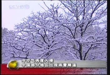
16Figure 2: Impression of the TRECVID 2005 training set. It contains videos from Ara-
bic, Chinese and English news channels. On news channels one can expect interviews,
speeches, stock market information, commercials, soap operas, sports, etc.
more useful to aggregate parts of the video into larger units. This aggregation does not
have to be based on entire frames per se. As in the CBIR field, it is possible to have a
finer granularity than an entire frame.
In general, camera shots are currently used as the fundamental units of video for
higher-level processing. In a video stream, boundaries between shots are defined at
locations where the author of the video makes a cut or transition to another scene or
a different camera and/or a jump in time. Fast shot boundary detectors with high
accuracy are available [32].
Given a shot segmentation of a video, the subsequent problem is the description of
these shots. The majority of current methods for extraction of visual descriptions uses
only a single keyframe which is representative for the entire shot. However, this can be
done under the assumption that other frames of the video will have similar content as
the keyframe. For action-packed shots, this assumption will not hold. The description
of the shot will then be incomplete. However, with the current state of technology, the
reduction in computational effort is more important. With a minimum shot duration of
two seconds and 25 frames per second, there is a fifty-fold reduction in processing time
(at a minimum).
In TRECVID 2005, the best performance on semantic concept detection for 7 con-
cepts has been achieved [33] using multiple global descriptions of color, shape, texture
and video motion. All visual descriptions, except for video motion, were performed on
the shot keyframe level. Text features based on a speech recognition transcription of
the video have also been used. While the contribution of individual features is undocu-
mented, for semantic concepts with strong visual cues, such as explosion, building and
mountain, the combination of features outperformed all other systems. The combination
of features is commonly referred to as fusion.
17Naphade [31] shows that multi-granular description of shot keyframes improves con-
cept detection over global description, similar to the results in Content-Based Image
Retrieval. Specifically, partitioning of keyframes with and without overlap and a rudi-
mentary form of interest regions are investigated.
In the video retrieval field, the focus lies on features which can be applied in a feasible
processing time. Features from the CBIR field are applied, investigating whether the
invariance properties improve retrieval results on extensive video datasets.
2.3 Conclusions
State-of-the-art in image descriptors such as the SIFT features for image retrieval do not
exploit the color information in an image: they operate on intensity information only.
Therefore, we will extend interest region detection and region description to include
color information. We evaluate our methods on concept detection in video, exploiting
the availability of large real-world datasets in the video retrieval field. To allow for
experimentation on a large dataset, we need fast feature extraction methods. Finally,
we will study the relative importance of using interest region detection over other image
areas by offsetting interest region description against global description.
183 Coloring concept detection using interest regions
In this chapter, we present the background information necessary for understanding our
concept detection system. In section 3.1, we introduce various digital image processing
methods and a reflection model to explain the physics behind images and video record-
ings. Using this model, several color spaces and their invariance properties are discussed
in section 3.2. In section 3.3, color constancy is discussed, which we use to achieve in-
variance to the color of the light source. In section 3.4, the use of image derivatives for
detection of edges and corners in an image is discussed. In section 3.5, interest point
detectors based on the Harris corner detector are used to detect scale invariant points.
For description of the image area around these points, we discuss several region descrip-
tors based on shape and color in section 3.6. In section 3.7, we discuss data clustering
algorithms which we use for data reduction. Finally, in section 3.8, machine learning
algorithms are discussed which we employ to learn models from annotated data.
3.1 Reflection model
It is important to understand how color arises, before we can discuss color-based features.
We need to understand the process behind the image formation process. Image formation
is modeled as the interaction between three elements: light, surface and observer (a
human observer or image capture devices such as cameras). In figure 3 the image
formation process is illustrated. Light from a light source falls upon a surface and is
reflected. The reflected light falls upon the sensor of the observer (human eye or camera
CCD chip) and eventually leads to a perception or measurement of color. Because we
will be processing digital videos, we will focus our discussion on the creation of digital
images and not on exploring human perception of color.
Figure 3: Image formation process. Light from a light source falls upon a surface and
is reflected. Depending on the angle between the surface normal and the incident light,
a different amount of light is reflected. The reflected light falls upon the sensor of an
observer which eventually leads to a perception or measurement of color.
Digital cameras measure the light that falls onto their CCD chip. This chip contains
many small sensors. These sensors have a sensitivity which varies depending on which
part of the light spectrum they are measuring. We will refer to the sensitivity of a sensor
at wavelength λ as f (λ). As there exists no single sensor which can accurately measure
the entire visible light spectrum, typical image capture devices sample the incoming
light using three sensors. In general, these sensors are sensitive to red, green and blue
wavelength light. The responses of these sensors are denoted by R, G and B. Together
they form a triplet of numbers. Mathematically, the responses are related to light,
19surface and sensor of the image formation process and are defined as follows:
R
R (~e · ~n) R E(λ)ρ(λ)fR (λ)dλ
G = (~e · ~n) E(λ)ρ(λ)fG (λ)dλ (1)
R
B (~e · ~n) E(λ)ρ(λ)fB (λ)dλ
with E(λ) the spectrum of the light source, ρ(λ) the reflectance of the surface and fS (λ)
the sensitivity of sensor S to different parts of the spectrum.
r
e
r
n
r
e
r
n
Figure 4: At the top, Lambertian reflectance of a surface is illustrated. Light penetrates
a surface and leaves the surface in all directions, reflected off of micro surfaces. This is the
color signal C(λ), which depends on the incident light E(λ) and the surface reflectance
ρ(λ). At the bottom, it is illustrated how a Lambertian surface, which reflects light
with equal intensity in all directions, can still have an intensity depending on the angle
between the surface normal ~n and the angle of incidence of the light ~e: the light per
unit area is different.
The color signal C(λ) which is perceived or measured by a sensor is created by light
E(λ) penetrating the surface and being reflected off of micro surfaces, depending on the
surface reflectance ρ(λ). This is illustrated in figure 4 at the top.
We assume surfaces are Lambertian, i.e. they reflect light with equal intensity in
all directions. This does not mean that all surfaces appear equally bright. The amount
of light arriving depends on the angle of the surface with respect to the light. This is
illustrated in figure 4 at the bottom. The intensity of the reflected light depends on
the cosine angle between the surface normal ~n and the angle of incidence of the light ~e.
We can write the scale factor (~e · ~n) outside the integral as it does not depend on the
wavelength of the light.
Digital images are created by taking color samples of a scene at many adjacent
locations. A pixel is the fundamental element in a digital image. With a pixel, a single
color is associated. A single pixel in this grid corresponds to a finite area of a digital
camera chip. Over this finite area R, G and B sensors are sampled. These samples are
combined into a RGB triplet, which is associated with a pixel. The RGB samples need
to be quantified within a limited range and precision to allow for digital storage. We
will assume a range of [0, 1] for the RGB triplet. RGB triplets include: (1, 0, 0) is red,
(0, 1, 0) is green, (0, 0, 1) is blue, (1, 1, 1) is white and (0, 0, 0) is black, (1, 1, 0) is yellow
and (1, 43 , 43 ) is pink.
203.1.1 Modelling geometry changes
Equation 1 shows that when the surface or lighting geometry changes, sensor responses
change by a single scale factor (~e · ~n). That means that sensor responses to a surface
seen under two different viewing geometries or illumination intensities are related by:
R2 sR1
=
R 2 + G2 + B 2 s(R2 + G2 + B2 )
It is straightforward to make the sensor responses independent of the light intensity,
by dividing by the sum of the R, G and B responses. This yields the normalized RGB
color space:
R
r R+G+B
g = G
R+G+B
(2)
b B
R+G+B
This yields the normalized RGB color model. The (r, g, b) triplet is invariant to changes
in geometry and illumination intensity, as the sum of the triplet is always equal to 1.
3.1.2 Modelling illumination color changes
When the color of the light source in a scene changes, it becomes very challenging to
achieve stable measures. A color measurement of the scene is needed which remains
stable regardless of the illuminant spectral power distribution E(λ). However, from
equation 1, we derive that the illumination E(λ) and the surface reflectance ρ(λ) are
heavily intertwined. Separating them is non-trivial.
However, often the relationship between sensor responses under different illuminants
can be explained by a simple model. This model is called the diagonal model or von
Kries model of illumination change [49]. In particular the responses to a single surface
viewed under two different illuminants 1 and 2 is approximated as:
R2 α 0 0 R1
G2 = 0 β 0 G1 (3)
B2 0 0 γ B1
where α = β = γ for geometry and illumination changes only.
The diagonal model only holds when there is no ambient lighting in the scene. Also, it
is assumed that a single spectral power distribution for the light source is used through-
out the scene. It is possible to use multiple light sources, as long as a single spectral
distribution E(λ) is sufficient to model them.
3.2 Color spaces and invariance
In this section we will discuss various color spaces which can be used to represent a color
and their invariance properties. Table 3 gives an overview of the invariance properties
of the color spaces based on Gevers [13]. The listed properties will not be repeated in
the text.
3.2.1 RGB
We have already encountered the RGB color space in our discussion on the image
formation process. The color space consists of three channels, R, G and B. Every
channel can take values in the range [0, 1]. In figure 5 the RGB color space is visualized
as an RGB cube. All grey-values lie on the axis (0, 0, 0) (black) to (1, 1, 1) (white).
21I RGB rgb H o1o2
viewing geometry - - + + +
surface orientation - - + + +
shadows/shading - - + + -
highlights - - - + +
illumination intensity - - + + +
illumination color - - - - -
Table 3: Overview of color spaces and their invariance properties based on Gevers [13].
+ denotes invariant and - denotes sensitivity of the color space to the imaging condition.
1
B
0
0
0
1 1 G
R
Figure 5: On the left a schematic view of the RGB color space. On the right a visual-
ization of the RGB color space. Only three faces of the RGB cube on the left can be
seen, containing red (1, 0, 0), green (0, 1, 0), blue (0, 0, 1), yellow (1, 1, 0), cyan (0, 1, 1),
magenta (1, 0, 1) and white (1, 1, 1). White is hard to discern due to the black lines of
the cube.
223.2.2 Normalized RGB
The normalized RGB color space is invariant to changes in lighting geometry and overall
changes in intensity. This was discussed in section 3.1.1. Equation 2 converts RGB
colors to normalized RGB.
The sum of r,g and b is always equal to 1, making one of the channels redundant.
It should come as no surprise then that the normalized RGB color space is equal to a
plane in the RGB color space: the plane where R + G + B = 1. In figure 6 the location
of this plane inside the RGB cube is visualized, as is the plane itself. This plane takes
the shape of a triangle. It is commonly referred to as the chromaticity triangle. White
(1, 1, 1) becomes ( 13 , 13 , 13 ) and is located at the center of the triangle. All values from
the grey-value axis (0, 0, 0) to (1, 1, 1) map to this point, except black, since division by
zero yields infinite values. Practical implementations of this color space do map black
to the point ( 13 , 13 , 13 ).
1
B
0
0
0
1 1 G
R
Figure 6: On the left the RGB cube. The chromaticity triangle ‘R + G + B = 1’ is
denoted by the dashed lines. On the right the chromaticity triangle is drawn separately,
visualizing the normalized RGB color space.
3.2.3 HSI
The HSI color space consists of three channels: Hue, Saturation and Intensity. In the
normalized RGB color space, the light intensity (R + G + B) was divided out. In the
HSI color space it is a separate channel:
R+G+B
I=
3
Hue and saturation are defined in the chromaticity triangle relative to a reference point.
This reference point is a white light source, located at the center of the triangle. Sat-
uration is defined as the radial distance of a point from the reference white point (see
figure 7). Saturation denotes the relative white content of a color.
r
1 1 1
S = (r − )2 + (g − )2 + (b − )2
3 3 3
Hue is defined as the angle between a reference line (the horizontal axis) and the
color point (see figure 7). Hue denotes the color aspect, e.g. the actual color:
1
r− 3
H = arctan 1
g− 3
231
B
0
0
0
1 1 G
R
Figure 7: On the left the RGB cube. The chromaticity triangle is denoted by the dashed
lines. The dotted line denotes the direction of the intensity channel: perpendicular to
the chromaticity triangle. On the right the chromaticity triangle is drawn separately,
denoting the meaning of hue and saturation channels. Hue and saturation are defined
for all planes parallel with the chromaticity plane; the specific plane depends on the
value of the intensity channel.
Figure 7 helps in understanding the HSI color space. The intensity channel is perpen-
dicular to the chromaticity triangle. Hue and saturation are most easily defined in the
chromaticity triangle. Note that the chromaticity plane’s location changes depending on
the intensity. This allows the HSI color model to cover the entire RGB cube. However,
hue and saturation are nonlinear. Saturation becomes unstable for low intensities. Hue
becomes unstable when saturation and intensity are low. This instability thus occurs
for grey-values and dark colors [46].
Above we have used normalized RGB channels in our conversion to HSI. A direct
conversion from RGB to HSI is as follows [19]:
√
3(G − B)
H = arctan
(R − G) + (R − B)
min(R, G, B)
S = 1−
R+G+B
R+G+B
I =
3
3.2.4 Opponent color space
The opponent color theory states that the working of the human eye is based on three
kinds of opposite colors: red-green, yellow-blue and white-black. An example of the
theory is the after-image. Looking at a green sample for a while will leave a red after-
image when looking at a white sample afterwards. The same effect occurs for yellow-blue.
Both members of an opponent pair exhibit the other: adding a balanced proportion of
red and green will produce a color which is neither reddish nor green. Also, no color
appears to be a mixture of both members of any opponent pair.
The opponent color space is based on the opponent color theory. It is given by:
R−G
o1 = √
2
R+G−2B
o2 = √
6
R+G+B
o3 = √
3
24The third channel o3 is equal to the intensity channel of HSI, subject to a scaling
factor. o1 and o2 contain color information. All channels of the opponent color space
are decorrelated.
3.3 Color constancy
Color constancy is the ability to recognize colors of objects invariant of the color of the
light source [10]. In the model of illumination color changes (section 3.1.2) corresponding
pixels of two images of a scene under two different illuminants are related by three
fixed scale factors. If we know the illuminant used in a scene and its relationship to a
predefined illuminant like RGB(1, 1, 1), then it is possible to normalize the scene and
achieve color constancy. Certain assumptions need to be made in order to achieve color
constancy. A number of different hypotheses are commonly used:
• Grey-World hypothesis [3]: the average reflectance in a scene is grey.
• White patch hypothesis [2]: the highest value in the image is white.
• Grey-Edge hypothesis [45]: the average edge difference in a scene is grey.
We will use the Grey-Edge hypothesis, because it outperforms the two other hy-
potheses [45]. With the Grey-Edge assumption the illuminant color can be computed
from the average color derivative in the image. For additional details we refer to [45].
Color constancy normalization gives invariance to color of the illuminant. From
equation 3 we derive that a division by the scaling factors α, β and γ achieves color
constancy. These scaling factors are equal to the estimated color of the illuminant when
converting to the illuminant RGB(1, 1, 1).
3.4 Image derivatives
The ability to take one or more spatial derivatives of an image is one of the fundamental
operations in digital image processing. However, according to the mathematical defini-
tion of derivative, this cannot be done. A digitized image is not a continuous function of
spatial variables, but a discrete function of the integer spatial coordinates. As a result
only approximations to the true spatial derivatives can be made.
Figure 8: Example image used to illustrate digital image processing operations through-
out this chapter. On the left the greyvalue version is shown. On the right the color
version is shown.
25The two dimensional Gauss filter is the most common filter for computing spatial
derivatives [14]. The linear Gaussian filter defined with the convolution kernel gσ is:
1 − x2 +y2 2
gσ (x, y) = e 2σ
2πσ 2
with σ the smoothing scale over which to compute the derivative. In the rest of this
thesis we will adopt the notation g(x, σ) for the Gaussian filter with x a 2D position
and σ the smoothing scale.
In figure 9 the first order derivatives of figure 8 in the x and y direction are shown
for different smoothing scales σ. These derivatives are referred to as Lx and Ly for the
x and y directions, respectively.
σD ≈ 1.07 σD ≈ 2.14 σD ≈ 4.28 σD ≈ 8.55
Lx
Ly
Figure 9: Image derivatives in the X direction Lx (top row) and in the Y direction
Ly (bottom row) at various differentiation scales. The differentiation scale is shown
above the column of the image. The derivatives have inverted and scaled for display.
White signifies a derivative value near 0. Black is the maximum derivative value, with
greyvalues lying in-between. Per scale the maximum derivative value is different: for
higher differentiation scales, the maximum value is lower. For visualization purposes,
these have been scaled to use the full grey-value range. The input image is shown on
the left in figure 8.
The image gradient at a point x is defined in terms of the first order derivatives as
a two-dimensional column vector:
Lx (x, σ)
5f (x) =
Ly (x, σ)
The magnitude of the gradient 5f is high at discontinuities in an image. Examples
are edges, corners and T-junctions. Using local maxima of the gradient magnitude it is
possible to build a very simple edge detector.
26A distinction between edges and corners and T-junctions can be made using the
second moment matrix (also known as auto-correlation matrix). The second moment
matrix µ is defined in terms of spatial derivatives Lx and Ly :
L2x (x, σD )
Lx Ly (x, σD )
µ(x, σD ) =
Lx Ly (x, σD ) L2y (x, σD )
with σD is the differentiation scale. Stability of the second moment matrix can be
increased by integrating over an area using the Gaussian kernel g(σI ) (see equation 4).
The eigenvalues of this matrix, λ1 (µ) and λ2 (µ), are proportional to the curvature
of the area around point x. Using the eigenvalues point x can be categorized as follows:
• λ1 (µ) ≈ 0 and λ2 (µ) ≈ 0: There is little curvature in any direction; the point is
located in an area of uniform intensity.
• λ1 (µ)
λ2 (µ): Large curvature in one direction and little curvature in the other
direction; the point is located on an edge.
• λ1 (µ) ≈ λ2 (µ)
0: Large curvature in both directions, the point is located on a
corner or a junction.
In the next section interest point detectors will be built using spatial derivatives and
the second moment matrix.
3.5 Interest point detectors
In this section we will discuss two scale invariant interest point detectors: Harris-Laplace
and ColorHarris-Laplace. Both are based on the Harris corner detector and use Lapla-
cian scale selection. For an overview of detectors see [24].
3.5.1 Harris corner detector
The Harris corner detector is based on the second moment matrix (see section 3.4). The
second moment matrix describes local image structure. By default the matrix is not
independent of the image resolution, so it needs to be adapted for scale changes.
The adapted matrix for a position x is defined as follows [27]:
L2x (x, σD )
2 Lx Ly (x, σD )
µ(x, σI , σD ) = σD g(σI ) (4)
Lx Ly (x, σD ) L2y (x, σD )
with σI the integration scale, σD is the differentiation scale and Lz (x, σD ) the derivative
computed in the z direction at point x using differentiation scale σD .
The matrix describes the gradient distribution in the local neighborhood of point
x. We compute local derivatives with Gaussian kernels with a size suitable for the
differentiation scale σD . The derivatives are averaged in the neighborhood of point x by
smoothing with a Gaussian window suitable for the integration scale σI .
The eigenvalues of the matrix represent the two principal signal changes in the neigh-
borhood of a point. This is akin to the eigenvalues of the covariance matrix in principal
component analysis (PCA). The eigenvalues are paired with a corresponding eigenvector.
We project the data onto the basis formed by the orthogonal eigenvectors. The eigen-
value corresponding to an eigenvector will then describe the variance in the direction of
the eigenvector.
We use this to extract points for which both eigenvalues are significant: then the
signal change is significant in orthogonal directions, which is true for corners, junctions,
27etc. Such points are stable in arbitrary lighting conditions. In literature these points
are called ‘interest points’.
The Harris corner detector [15], one of the most reliable interest point detectors,
is based on this principle. It combines the trace and the determinant of the second
moment matrix into a cornerness measure:
cornerness = det(µ(x, σI , σD )) − κtrace2 (µ(x, σI , σD )) (5)
with κ an empirical constant with values between 0.04 and 0.06.
Local maxima of cornerness measure determine the location of interest points. The
interest points detected depend on the differentiation and integration scale. Due to the
definition of cornerness, it is possible for the measure to become negative, yet still be
a maximum. This happens if all values surrounding the negative maximum have lower
values than the maximum. To counter very low cornerness maxima, they are only
accepted if they exceed a certain threshold.
original image σI = 1.5 σI = 3 σI = 6 σI = 12
Figure 10: Corners (red dots) detected at different scales using Harris corner detector.
The differentiation scale σD has a fixed relation to the integration scale: σD = 0.7125σI .
The differentiation scales match those displayed in figure 9. On the left the input image
is shown.
3.5.2 Scale selection
The Harris corner detector from the previous section has scale parameters. The detected
points depend on this scale. It is possible for a single point to be detected at multiple
(adjacent) scales.
The idea of automatic scale selection is to select the characteristic scale of the point,
depending on the local structure around the point. The characteristic scale is the scale
for which a given function attains a maximum over scales.
It has been shown [26] that the cornerness measure of the Harris corner detector
rarely attains a maximum over scales. Thus, it is not suitable for selecting a character-
istic scale. The Laplacian-of-Gauss (LoG) does attain a maximum over scales. We use
it to select the characteristic scale of a point. With σn , the scale parameter of the LoG,
it is defined for a point x as:
|LoG(x, σn )| = σn2 |Lxx (x, σn ) + Lyy (x, σn )| (6)
In figure 11, the LoG kernel is visualized. The function reaches a maximum when the
size of the kernel matches the size of the local structure around the point. It responds
to blobs very well due to its circular symmetry, but it also responds to corners, edges,
ridges and junctions.
28−3
x 10
1
0
−1
−2
−3
−4
25
20 25
15 20
10 15
10
5
5
0 0
Figure 11: Laplacian-of-Gauss (LoG) kernel. The kernel shown has scale σn = 5.
3.5.3 Harris-Laplace detector
The Harris-Laplace detector uses the Harris corner detector to find potential scale-
invariant interest points. It then selects a subset of these points for which the Laplacian-
of-Gaussian reaches a maximum over scale.
Mikolajczyk [27] defines an iterative version of the Harris-Laplace detector and a
‘simplified’ version which does not involve iteration. The simplified version performs a
more thorough search through the scale space by using smaller intervals between scales.
The iterative version relies on its convergence property to obtain characteristic scales.
By performing iteration, it gives more fine-grained estimations. Mikolajczyk notes that
the ‘simplified’ version is a trade-off between accuracy and computational complexity.
Due to our need for fast feature extraction (section 2.3), we will use the simplified version
of the Harris-Laplace detector.
In section 5.2 we will discuss the Harris-Laplace algorithm and its implementation
in more detail.
3.5.4 Color boosting
The intensity-based interest point detector in the previous section uses the derivative
structure around points to measure the saliency of the point. Stable points with high
saliency qualify as an interest point. In the next section interest points detectors will
be extended to use all RGB channels.
Rare color transitions in an image are very distinctive. By adapting the saliency of
an image, the focus of the detector shifts to more distinctive points. The transformation
of the image to achieve this is called color saliency boosting. We use the color boosting
transformation in the opponent color space [44]. This transformation is a weighing of
29the individual opponent channels:
o10 = 0.850 o1
o20 = 0.524 o2
o30 = 0.065 o3
where the sum of the squared weights is equal to 1. These weights are focused on the
red-green and yellow-blue opponent pair, with almost no weight given to the intensity
o3 channel. Figure 12 (on the left) shows the colorboosted version of the color image in
figure 8. The difference between the glass and the background has increased significantly,
increasing saliency of the edges of the glass.
3.5.5 ColorHarris-Laplace detector
So far the images consist of single channels, i.e. intensity images. Only the Harris corner
detector and the LoG function operate on the image directly. In this section, we extend
them to operate on color images.
The Harris corner detector uses the second moment matrix. The elements of the
matrix are always the product two image derivatives Lx (with x the derivative direc-
tion). For the extension to multiple channels n, we replace Lx with a vector f~x =
Cn T
LC C2
x , Lx , . . . , Lx
1
with Ci the ith channel. The product between derivatives is re-
placed with a vector inproduct. If the vector is 1-dimensional (e.g. an intensity image),
this is equivalent to the original second moment matrix.
The second moment matrix for a ColorHarris corner detector is:
!
2 f~x (x, σD ) · f~x (x, σD ) f~x (x, σD ) · f~y (x, σD )
µRGB (x, σI , σD ) = σD g(σI )
f~x (x, σD ) · f~y (x, σD ) f~y (x, σD ) · f~y (x, σD )
Cn T
with f~x = LC C2
x , Lx , . . . , Lx
1
for an image with channels {C1 , C2 . . . Cn }, with LC
x
i
th
being the Gaussian derivative of the i image channel Ci in direction x. The image
channels Ci can be instantiated to channels of any color model. However, it is also
possible to first apply preprocessing operations (such as color boosting) to an image and
then instantiate the channels. For our ColorHarris corner detector, we instantiate the
channels to the R, G and B channels of the standard RGB color space. We preprocess
images using color boosting. Results of this detector are shown in figure 12. Due to color
boosting, the cloth underneath the glass now consists of different shades of blue only.
The contribution of the R and G channels to the cornerness will be very low because
there is almost no change in these channels in the cloth. Primarily, the cornerness
comes from the B channel only, which by itself is not enough to exceed the threshold.
One way to extend the Laplacian-of-Gaussian kernel to multiple channels is by sum-
ming the responses of the individual channels:
|LoGRGB (x, σn )| = |LoGR (x, σn )| + |LoGG (x, σn )| + |LoGB (x, σn )|
It is also possible to assign different weights depending on the color channel or to
use different color channels altogether.
In conclusion, we have two different scale invariant point detectors. Harris-Laplace
triggers on corners in an intensity image, while Colorboosted ColorHarris-Laplace fo-
cuses on the color information in an image.
30You can also read