DOCTORAL THESIS IN PHYSICS - KTH ROYAL INSTITUTE OF TECHNOLOGY - DIVA
←
→
Page content transcription
If your browser does not render page correctly, please read the page content below
kth royal institute
 of technology

 Doctoral Thesis in Physics

 Peripheral Optics of the Human Eye:
 Applied Wavefront Analysis
 DMITRY ROMASHCHENKO

Stockholm, Sweden 2021
Peripheral Optics of the Human Eye:
Applied Wavefront Analysis
DMITRY ROMASHCHENKO

Academic Dissertation which, with due permission of the KTH Royal Institute of Technology,
is submitted for public defence for the Degree of Doctor of Philosophy on Friday the 22nd of
January 2021 at 1:00 pm i FA32, Albanova University Center, Roslagstullsbacken 21, Stockholm.

Doctoral Thesis in Physics
KTH Royal Institute of Technology
Stockholm, Sweden 2021
© Dmitry Romashchenko

Cover page photo: Anna Grigoreva

ISBN 978-91-7873-735-2
TRITA-SCI-FOU 2020:46

Printed by: Universitetsservice US-AB, Sweden 2020
iii

Abstract

This thesis is dedicated to implementing wavefront analysis for studying
the peripheral optics of the human eye with an emphasis on its relation to
myopia. The aim is to find properties in the peripheral image quality. The
work consists of the following main parts:
 • Literature review and analysis of population data on ocular aberra-
 tions of the relaxed eye over the horizontal visual field (Paper B). This
 paper recommends a method for the peripheral wavefront analysis and
 presents data for different groups of people: (a) population average,
 (b) myopic, and (c) emmetropic subjects.
 • Development of a novel, dual-angle, open field wavefront sensor (Paper
 D). The device enables recording of real-time, simultaneous foveal-
 peripheral wavefront measurements, while providing a binocular open
 field of view.
 • Studying optical quality for myopic and emmetropic subjects under
 different accommodation demands (Paper F). The novelty of this work
 is the real-time accommodation state tracking, allowing a more accu-
 rate data analysis of both the dynamic and the average foveal and
 peripheral optical quality.
 • Using wavefront analysis to understand the contribution of optics to
 different aspects of peripheral human vision, such as resolution acuity
 and contrast sensitivity (Papers A, C, E).
The results obtained in this work show the benefit of binocular viewing and
real-time foveal measurements when studying peripheral aberrations under
accommodation. With increasing accommodation, the relative peripheral
refraction of myopic eyes becomes more negative, while the changes for the
emmetropic eyes are small. However, the total peripheral optical quality
proved to be similar between myopic and emmetropic subjects and varied
little between distant and near objects. The results also suggest that the
accommodative response is not the leading factor defining the magnitude
of the microfluctuations in accommodation. Peripheral low contrast vision,
irrespective of the foveal refractive error, is demonstrated to improve when
monochromatic aberrations are corrected, while the effects of chromatic
aberrations are negligible. Finally, the myopia control MiSight® multifocal
contact lenses are shown to reduce vision performance in accommodation
as well as in peripheral low-contrast resolution.
iv

Sammanfattning

I denna avhandling används vågfrontsanalys för att studera ögats perifera
optik med betoning på dess betydelse för utvecklingen av närsynthet (myo-
pi). Syftet är att hitta egenskaper i den perifera bildkvalitén som skulle
kunna användas av ögat för att reglera dess tillväxt. Avhandlingsarbetet
består av följande delar:
 • Litteraturgenomgång och analys av populationsdata på det oackom-
 moderade ögats perifera optik över det horisontella synfältet (artikel
 B). Denna översiktsartikel beskriver en metod för att analysera peri-
 fer vågfrontsdata och presentera sammanställd data för olika grupper:
 (a) populationsmedelvärden, (b) närsynta och (c) rättsynta.
 • Utveckling av en ny typ av vågfrontssensor med öppet synfält och
 dubbla kanaler (artikel D). Detta instrument möjliggör tidsupplösta
 och simultana mätningar av de centrala och perifera vågfrontsfelen i
 realtid med ett öppet binokulärt synfält.
 • Undersökning av den optiska kvalitén i närsynta och rättsynta ögon
 vid olika ackommodationsnivåer (artikel F). Det unika i detta arbete
 är att ögats ackommodationstillstånd följs i realtid vilket ger utökade
 möjligheter till noggrann analys av både dynamik och medelvärden
 hos den centrala och perifera optiska kvalitén.
 • Användning av vågfrontsanalys för att klargöra optikens betydelse för
 olika perifera synkvalitéer, så som synskärpa och kontrastkänslighet
 (artikel A, C, E).
Resultaten av dessa studier visar på fördelen med binokulärt synfält och si-
multana centrala mätningar när perifera aberrationer undersöks vid ackom-
modation. Den relativa perifera refraktionen blir mer negativ med ökande
ackommodation för de närsynta ögonen, medan förändringarna i de rätt-
synta ögonen är små. Den totala perifera optiska kvalitén var dock likartad
för både närsynta och rättsynta och varierade knappt mellan avlägsna och
närliggande objekt. Mätningarna indikerar även att ögats ackommodations-
nivå inte är den huvudsakliga orsaken till storleken på mikrofluktuationer
i ackommodationen. Oberoende av centralt brytningsfel, visade det sig att
perifer lågkontrastsyn förbättras med korrektion av monokromatiska aber-
rationer, men att effekten av kromatiska aberrationer är försumbar. Slut-
ligen visar studierna att multifokala kontaktlinser som utformats för att
bromsa närsynthet, MiSight® , försämrar synfunktionen både vad gäller ac-
kommodation och perifer lågkontrastresolution.
v

List of Papers

Paper A
A. P. Venkataraman, P. Papadogiannis, D. Romashchenko, S. Winter, P.
Unsbo, L. Lundström, ”Peripheral resolution and contrast sensitivity: effect
of monochromatic and chromatic aberrations”, J. Opt. Soc. Am. A 36(4),
B52-B57 (2019).

Paper B
D. Romashchenko, R. Rosén, L. Lundström, ”Peripheral refraction and
higher order aberrations”, Invited review, Clin. Exp. Optom. 103(1),
86-94 (2020).

Paper C
P. Papadogiannis, D. Romashchenko, P. Unsbo, L. Lundström, ”Lower
sensitivity to peripheral hypermetropic defocus due to higher order ocular
aberrations”, Ophthalmic Physiol. Opt. 40(3), 300-307 (2020).

Paper D
D. Romashchenko and L. Lundström, ”Dual-angle open field wavefront
sensor for simultaneous measurements of the central and peripheral human
eye”, Biomed. Opt. Express 11(6), 3125–3138 (2020).

Paper E
P. Papadogiannis, D. Romashchenko, S. Vedhakrishnan, B. Persson, A.
Lindskoog-Pettersson, S. Marcos, L. Lundström, ”Foveal and peripheral
visual quality and accommodation with multifocal contact lenses”, in
manuscript.

Paper F
D. Romashchenko, P. Papadogiannis, P. Unsbo, L. Lundström, ”Foveal-
peripheral real-time aberrations with accommodation in myopes and em-
metropes”, in manuscript.
vi

Contents

Abstract iii

Sammanfattning iv

List of Papers v

List of Acronyms ix

1 Introduction 1

2 The Human Eye 5
 2.1 Optics of the Human Eye . . . . . . . . . . . . . . . . . . . . 5
 2.1.1 Accommodation . . . . . . . . . . . . . . . . . . . . . 6
 2.1.2 Central and Peripheral Retina . . . . . . . . . . . . . 8
 2.1.3 Visual Acuity . . . . . . . . . . . . . . . . . . . . . . . 9

3 Describing an Ocular Optical System 11
 3.1 Reduced Eye Model and Refractive Errors . . . . . . . . . . . 11
 3.2 Schematic Eye Models . . . . . . . . . . . . . . . . . . . . . . 13
 3.3 Anatomically Accurate Eye Models . . . . . . . . . . . . . . . 13
 3.4 The “Black Box” Approach of Wavefront Analysis . . . . . . 14
 3.4.1 Zernike Polynomials for Wavefront Representation . . 14
 3.4.2 Calculating Refractive Errors Using Zernike Polyno-
 mials . . . . . . . . . . . . . . . . . . . . . . . . . . . . 16
 3.4.3 Recalculating Zernike Coefficients for Different Wave-
 lengths . . . . . . . . . . . . . . . . . . . . . . . . . . 18
 3.4.4 Point Spread Function (PSF) and Modulation Trans-
 fer Function (MTF) . . . . . . . . . . . . . . . . . . . 19
 3.4.5 Contrast Sensitivity Function (CSF) . . . . . . . . . . 23
 3.4.6 Other Retinal Image Metrics . . . . . . . . . . . . . . 24

4 Instrumentation for the Wavefront Measurements 27
vii

 4.1 Hartmann-Shack Wavefront Sensor . . . . . . . . . . . . . . . 27
 4.2 Adaptive Optics Vision Simulator . . . . . . . . . . . . . . . . 28
 4.3 Dual-angle Open Field Wavefront Sensor . . . . . . . . . . . . 30
 4.3.1 Measuring Accommodative Lag with the Dual-angle
 Sensor . . . . . . . . . . . . . . . . . . . . . . . . . . . 31
 4.3.2 Measuring Accommodation Microfluctuations with
 the Dual-angle Sensor . . . . . . . . . . . . . . . . . . 32

5 Applications: Peripheral Aberrations 33
 5.1 Population Average Aberrations across the Horizontal Visual
 Field . . . . . . . . . . . . . . . . . . . . . . . . . . . . . . . . 33
 5.1.1 MTF Calculations for the Human Eye . . . . . . . . . 35
 5.2 Synchronized Foveal-peripheral Wavefront Measurements for
 Different States of Accommodation . . . . . . . . . . . . . . . 39
 5.2.1 Higher Order Aberrations . . . . . . . . . . . . . . . . 39
 5.2.2 Accommodation Microfluctuations . . . . . . . . . . . 40
 5.2.3 MTF as a Function of Accommodation . . . . . . . . . 41

6 Applications: Peripheral Vision 43
 6.1 Psychophysical Vision Evaluation . . . . . . . . . . . . . . . . 43
 6.2 Effects of Aberrations on Peripheral Vision . . . . . . . . . . 44
 6.3 Effect of Aberrations on Peripheral Sensitivity to Positive
 and Negative Defocus . . . . . . . . . . . . . . . . . . . . . . 45

7 Peripheral Vision, Aberrations, and Myopia Research 47
 7.1 Role of Peripheral Vision in Myopia Research . . . . . . . . . 47
 7.2 Ocular Aberrations in Myopic and Non-myopic Eyes . . . . . 49
 7.2.1 Relative Peripheral Refraction . . . . . . . . . . . . . 49
 7.2.2 Higher Order Aberrations . . . . . . . . . . . . . . . . 51
 7.3 Vision and Aberrations with Multifocal Contact Lenses . . . 52

8 Conclusions and Outlook 55

Supplementary 57

References 59

Acknowledgements 67

Summary of the Original Work 69
ix

List of Acronyms

AMFs Accommodation Microfluctuations
CSF Contrast Sensitivity Function
D Diopters, 1/m
HOA Higher Order Aberrations
HSWS Hartmann-Shack Wavefront Sensor
LCOS SLM Liquid Crystal On Silicon Spatial Light Modulator
MAR Minimum Angle of Resolution
MTF Modulation Transfer Function
NCSF Neural Contrast Sensitivity Function
OTF Optical Transfer Function
PSF Point Spread Function
RPR Relative Peripheral Refraction
SE Spherical Equivalent
VA Visual Acuity
VF Visual Field
INTRODUCTION | 1

Chapter 1

Introduction

Vision plays an important role in our life. Most of our everyday activities
would be much harder without real-time information from the whole extent
of our visual field (VF). For a human, the binocular field of view is approx-
imately 200° horizontally and 150° vertically. The central vision subtends
a cone of about 5° in diameter. The size of this area corresponds to the
fovea – a part of the retina with the highest density of photoreceptors and
sharpest image in the eye. Foveal vision is used for tasks that require resolu-
tion of fine details and objects identification (for example, reading). As we
move outside the fovea (see Figure 1.1), the quality of the image, formed on
the retina, gets worse. The primary responsibility of the corresponding VF,
however, also gradually changes from the high resolution tasks in the fovea

 Figure 1.1. Horizontal binocular visual field of a human eye.
2 | INTRODUCTION

to the low contrast object detection in the periphery. Thus, peripheral vi-
sion is responsible for awareness of a person’s surroundings; without it many
everyday activities (for example, driving) would be impossible. Given the
importance of vision, any deterioration in its performance have a noticeable
effect on our lifestyle.
 The main purpose of the visual optics research is prevention, diagno-
sis, treatment, and maximizing functionality in the presence of any vision
degradation. Such a task of course requires in-depth understanding of the
vision mechanisms, which makes visual optics a cross-disciplinary biomedi-
cal research field.
 Vision as a process can be split into two complementary parts: (1)
creating an image on the retina and (2) processing this image. The first
part is governed by the optical system of the eye. The second one involves
complex interactions along the whole path from the retina to the brain. The
measurements of the ocular optics require in situ optical system diagnostics.
The neural processing is usually studied with psychophysical methods.
 Some of the most important applications of visual optics research are:

 • Vision aid. This is probably the most prevalent application of the
 knowledge in optics of the human eye. It includes simple sphero-
 cylindrical correction (for far-sightedness, near-sightedness, and astig-
 matism), bifocal and progressive spectacles (for presbyopia), and op-
 tical aid for patients with low vision (for example, due to age-related
 macula degeneration).

 • Diagnostics of vision. Measurements of optics of the eye are daily
 used to diagnose common ocular conditions (such as nearsightedness,
 farsightedness, and astigmatism) and more severe ones (such as ker-
 atoconus). In the recent years, these measurements are also used in
 attempts to early-identify subjects with high risk of developing near-
 sightedness.

 • Near-sightedness (myopia) interventions. Myopia is a global
 problem with a rising prevalence attracting more and more research
 interest. Knowledge of the human eye optics is used to design effective
 myopia prevention and control interventions.

 • Ocular surgery. Nowadays ocular surgery is used very widely. Many
 of the performed tasks require careful measurements of the ocular
 optics before, after or during the surgery. The two most typical of
 these tasks are (1) replacing crystalline lens for an intra-ocular lens
 in cataract surgery and (2) laser surgery for near- and far-sightedness
 treatment.
INTRODUCTION | 3

 The focus of this work is directed towards the peripheral optical system
of the human eye and its effects on vision. The basic anatomical background
is complemented by comparing several practical approaches to represent
ocular optics. This is followed by the description of two optical setups that
use one of the most common measurement techniques nowadays, namely
wavefront sensing. The final parts concern some practical methods of data
processing and analysis as well as their further applications, especially in
relation to myopia.
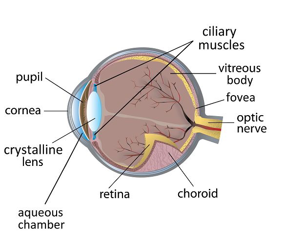
THE HUMAN EYE | 5

Chapter 2

The Human Eye

2.1 Optics of the Human Eye

The human eye optical system is a sophisticated mechanism. Figure 2.1
shows a schematic drawing of the human eye. Its total axial length, around
23 mm, is divided between cornea, aqueous chamber, crystalline lens, and
vitreous body. The main purpose of the optical system is to create a sharp
image on the retina that can be further processed by the neural channels.
The total optical power of the eye, on average, is +60 D which corresponds
to back focal length of 22.27 mm and refractive index of 1.336. This power
is split between the cornea and the crystalline lens.
 The cornea provides around 2/3 of the optical power of the eye. It is a

 Figure 2.1. Schematic drawing of the human eye showing its main components
 [1].
6 | THE HUMAN EYE

rather thin (550 m) structure shaped as a meniscus lens. The five main
layers of the cornea are: epithelium, Bowman’s layer, stroma, Decsemet’s
membrane, and endothelium [2]. The thickest of these are the epithelium (50
 m) and the stroma (440-470 m) [2]. The stroma is particularly interesting
for vision research as it is this layer that is reshaped in sight-correcting
surgeries, such as PRK, LASIK and SMILE. Although the cornea consists
of layers with different refractive indexes [3, 4], for most applications it is
sufficient to use an average refractive index of 1.37.
 The residual 1/3 of the ocular optical power is provided by the crystalline
lens. It is much thicker than the cornea: 4 mm [5] compared to 0.55 mm
(center thickness). In cross-section, the crystalline lens is shaped as a prolate
ellipse with its longer axis oriented perpendicular to the optical axis of the
eye (see Figure 2.1). It has a structure of a thin elastic shell filled with
a gel-like gradient refractive index core. The optical density of the core is
highest in the center and gradually decreases towards the shell (see Figure
2.2a). This gradient refractive index renders negative spherical aberration
in the positive-power crystalline lens [6]. That is, the marginal rays are
focused further away from the lens than the paraxial rays. The negative
spherical aberration of the lens partially compensates the positive spherical
aberration of the cornea [6]. Similar to the cornea, in some applications it
is sufficient to simplify the true refractive index of the lens using a constant
value across the whole volume.

 (a) (b)

 Figure 2.2. a - schematic drawing of the crystalline lens gradient refractive index.
 The refractive index is lowest at the cortex (1.37) and highest at the core of the
 lens (1.41). Data from Kasthurirangan et al. [7]. b – schematic drawing of the
 change in the shape of the crystalline lens during accommodation.

2.1.1 Accommodation
Accommodation is the mechanism to increase the optical power of the eye
so that the objects at different distances are imaged sharply on the retina.
THE HUMAN EYE | 7

This is possible by means of the crystalline lens. When looking at far, the
relaxed ciliary muscle is “stretching” the crystalline lens (see Figure 2.1).
When looking at near, the ciliary muscle is moving towards the optical axis,
relaxing the tension on the lens. The lens then is reshaped to a more oblate
form (Figure 2.2b). During accommodation, the gradient of the refractive
index follows the same pattern irrespective of the lens shape: highest in the
center and lower at the edge [7].
 Accommodative response is the increase in the optical power of the eye
during accommodation, measured in diopters. Accommodative demand is
the required value of the accommodative response, set by the distance to
the target,that would create the sharpest image of the viewed object on the
retina. It is not rare that the accommodative response of the eye is not
perfectly equal to the accommodative demand from the target.
 Accommodation lag describes the case when the accommodative response
is lower than the accommodative demand. Accommodation lead describes
the opposite case: the response is higher than the demand. Accommoda-
tive lag is quite common when viewing targets requiring high amounts of
accommodation. In order to reduce the strain on the ciliary muscle the eye
somewhat reduces the accommodative response. The retinal image is then
not perfectly focused but still has decent quality. The magnitude of the
accommodative lag depends both on the parameters of the eye and on the
viewing target. Optical errors of the eye can expand the depth of field which
would reduce the demand on focusing of the retinal image. Furthermore,
the pupil constriction, which is naturally triggered when an eye accommo-
dates [8], can also increase the depth of focus. However, during a steady
fixation the pupil diameter may to some extant enlarge back to the more
habitual and preferred diameter [9]. On the other hand, increase in the
pupil diameter leads to an increased blur by the ocular aberrations. As for
the viewing target, the features observed from a close distance are usually
large. And the apparent contrast of large features is less sensitive to defocus
in comparison to the small features.
 Accommodation microfluctuations (AMFs) are small variations in the
optical power of the eye during a steady fixation. Their magnitude, mea-
sured as the standard deviation of the accommodative response, can reach
up to 0.5 D [10]. It is also highly dependent on the subject and the visual
task. In particular, the magnitude has been shown to increase with (a)
increase in accommodative response [11, 12], and (b) decrease in the (artifi-
cial) pupil diameter under a steady state accommodation [11, 13, 14]. Some
previous work also suggests that the dependence on the accommodative re-
sponse is not linear: the AMFs reach their amplitude peak at intermediate
accommodation response of about 3-5 D [15].
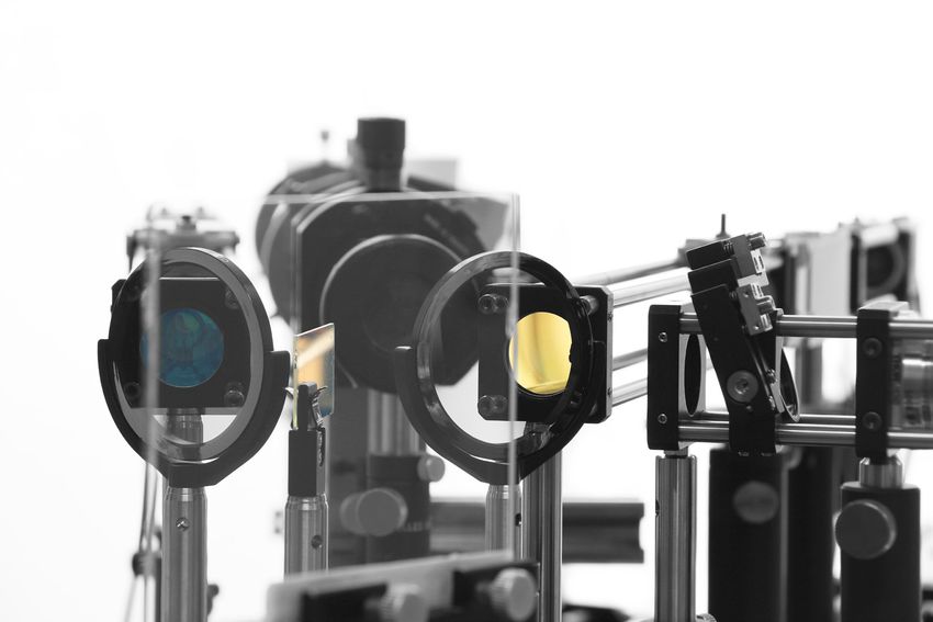
8 | THE HUMAN EYE

2.1.2 Central and Peripheral Retina
The detection of the image on the retina is possible by means of photorecep-
tors: cones and rods. These photoreceptors, although performing similar
tasks, are quite different in their parameters.
 In the human eye there are approximately six million cones. The density
of cones is highest in the fovea and is reducing for the off-axis angles. The
diameter of the cones’ inner segment is 2 m in the fovea and is enlarging
up to 8 m further out in the periphery [16]. The cones are fully utilized
in photopic luminance conditions (> 1 / 2 ) to detect high-resolution
color images. The color vision is possible due to the presence of three
different types of cones: short- (S), medium- (M) and long- (L) wavelengths
sensitive with their spectral sensitivity peaks at 420 nm, 534 nm, and 564
nm respectively (Figure 2.3).
 In the retina there are much more rods than cones: 120 million (com-
pared to six million). There are no rods in the central fovea, and their
density grows towards the periphery. The inner segment diameter of the
rods is less than 2 m [16]. They are most efficient at scotopic luminance
levels (< 10−3 / 2 ). Their spectral sensitivity has a peak at 498 nm
(Figure 2.3).
 When light is absorbed by the rods and the cones, the signal does not
travel directly to the brain. Instead, it undergoes additional pre-processing
in the retina by horizontal, bipolar, and amacrine cells and, finally, reaches
the ganglion cells (see Figure 2.4). Each ganglion cell has a direct channel
through the optic nerve to the visual cortex. Such a complex retinal struc-
ture allows to gain a lot of information already at the retinal level, including
contrast and color [18]. In this architecture the input for one ganglion cell
can come either from one photoreceptor or from a group of photoreceptors.

 Figure 2.3. Relative sensitivity curves of cones and rods. Data from [17].
THE HUMAN EYE | 9

That is, one signal, that goes to the brain, can describe combined output
from several rods and cones.
 The sampling of the retina is defined by the size of the retinal receptive
fields. A retinal receptive field is an area of photoreceptors, connected to
one ganglion cell. In the fovea, where each cone has its “own” ganglion
cell, the receptive field size is equal to the cone size. When moving towards
the periphery, the receptive field enlarges, meaning that there are multiple
photoreceptors connected to one ganglion cell. The retinal receptive field
size is thus larger compared to the fovea [19].
 The shape of the receptive fields agrees with the quality of the ocular
optics over the retina relatively well. In the absence of refractive errors (see
Chapter 3), the foveal image quality is the sharpest throughout the eye: it
corresponds to the smallest possible retinal receptive field size. Further out
in the periphery, the retinal image quality, including the resolution, becomes
worse. This is mirrored by the larger sizes of the corresponding receptive
fields that provide coarser sampling compared to the fovea. Also, periph-
eral retinal image is subject to off-axis astigmatism: the optical quality is
better in the tangential plane and worse in the sagittal plane. The periph-
eral receptive fields are also repeating this shape being more elongated in
the radial directions. This creates an asymmetry in the peripheral vision
performance known as the meridional effect [20–22].

 Figure 2.4. Illustration of the retinal architecture.

2.1.3 Visual Acuity
Visual acuity (VA), or resolution acuity, refers to the size of the smallest
perceivable feature for a 100% object contrast. It is probably the most
intuitive visual performance metric. Ultimately, the resolution is limited by
the size of the retinal receptive fields.
10 | THE HUMAN EYE

 The VA is mostly measured by means of charts that contain letters of
different sizes and are supposed to be viewed from a fixed distance (see
Figure 2.5). The results of these measurements are called the letter VA,
in contrast to the grating VA. The standard for the viewing distance for
the letter charts is 6 m or 20 ft. Normal VA is considered as the ability
to resolve a letter subtending 5 minutes of arc. Such letter stroke width
is eqivalent to the Minimum Angle of Resolution (MAR) equal to 1 (see
 1
Figure 2.5). The VA can then be calculated as = . Thus, normal

vision gives = 1 with > 1 being better and < 1 being worse.
 There are more ways to assess VA. It can be measured as ( )
as well as in terms of spatial frequency (see Section 3.4.4). The = 1
corresponds to the spatial frequency of 30 cycles/degree. Alternatively, the

VA is also often denoted as a fraction 0 , where 0 is the MAR that

corresponds to the normal VA, and the A is the MAR measured for the
 6 20
real eye. This VA fraction can be written in the forms and , where

the numerators are chosen to depict the viewing distances of 6 m and 20 ft
respectively. Nowadays, all of the described notations can be seen.

 Figure 2.5. Illustrations to the definitions of the Visual Acuity [23].
DESCRIBING AN OCULAR OPTICAL SYSTEM | 11

Chapter 3

Describing an Ocular Optical
System

The previous chapter has described the complexity of the optical compo-
nents of the human eye. A model of this system, that includes all anatomic
features, would be laborious both to obtain and to use. In practice, this
system is simplified by different approximations that reduce the number of
described features but still keep the model suitable for various applications.
This chapter describes four models that use different levels of approximation
for the optics of the eye.

3.1 Reduced Eye Model and Refractive Errors

The simplest representation of the eye’s optics is given by a reduced eye
model. It is based on paraxial approximation. This model implies that
the eye has a uniform refractive index and only one refractive surface, the
cornea, that provides the whole optical power of the eye. The entrance pupil
as well as the principal points are then also located at the corneal surface.
Accommodation in the reduced eye model can be described as optical power
additional to that of the cornea. A population average reduced eye can be
illustrated by the Emsley reduced eye model [24] with optical power of 60
D, corneal radius of 5.555 mm, refractive index of 1.333, and axial length
of 22.222 mm.
 The reduced eye models can be somewhat customized and are finding a
broad application in optometry, in particular to describe the refractive errors
of the eye. Refractive errors include myopia (near-sightedness), hyperme-
tropia (far-sightedness), and astigmatism. An eye that has no refractive
errors is called emmetropic. Such an eye in its relaxed state (no accommo-
dation) can create a sharp retinal image of an infinitely far object (Figure
12 | DESCRIBING AN OCULAR OPTICAL SYSTEM

3.1, top-left). Myopia is a condition when the optical power of the relaxed
eye is too large for its axial length. Therefore, an image of the infinitely far
object is located in front of the retina (Figure 3.1, bottom-left). The most
common reason for myopia is that the eye globe growing too long. In con-
trast, with hypermetropia the optical power of the eye is too low for its axial
length. The image of the far-away object is thus created behind the retina
(Figure 3.1, top-right). Finally, astigmatism describes a case when the opti-
cal power varies for different different meridians (Figure 3.1, bottom-right).
The meridians of highest and lowest optical power are perpendicular to each
other. The most commonly occurring with the rule astigmatism means that
the vertical meridian has the highest optical power. The opposite case, when
the highest optical power is in the horizontal meridian, is called against the
rule astigmatism. An astigmatism where the highest optical power is neither
in the horizontal nor in the vertical meridian is called oblique astigmatism.
 The refractive errors are defined by the dioptric power of the corrective
lenses needed to make a particular eye emmetropic. Myopia and hyperme-
tropia are uniform in all ocular meridians and are therefore corrected with
spherical lenses. Astigmatism, on the other hand, requires cylindrical lenses
for its correction. By Swedish convention, refractive error of central vision is
given as Spherical lens power / Cylindrical lens power x Axis (for example,
-3.00/-0.75 x 10). Here the powers are in diopters and the cylindrical power
is always negative. The axis of the cylindrical lens is measured in degrees
from the horizontal meridian. It is worth emphasizing that “axis” refers to
the axis of rotation for the lens’s refractive surface. Thus, the meridian that

 Figure 3.1. Illustration of the refractive errors in a reduced eye for an infinitely
 far on-axis object. Top-left - emmetropia; bottom-left - myopia; top-right -
 hypermetropia; bottom-right - astigmatism
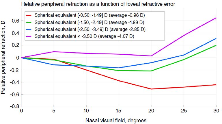
DESCRIBING AN OCULAR OPTICAL SYSTEM | 13

has the optical power is perpendicular to the axis of the cylinder.
 The approach of refractive errors is also applied for the peripheral VF.
In this case there is an additional concept – Relative Peripheral Refraction
(RPR). This is the peripheral spherical refractive error relative to that in
the fovea. In other words, it shows the defocus of the peripheral retinal
image when the foveal refractive error is corrected. The RPR can therefore
be compared between subjects with different central refractive errors.

3.2 Schematic Eye Models

The schematic eye models are more complex than the reduced ones. They
include at least three refractive surfaces: one for the cornea and two for
the crystalline lens. Unlike in the reduced models, the surfaces here can be
aspheric, and the refractive index can incorporate gradient.
 One of these schematic models, the Navarro eye model [25], is presented
in the Supplementary. The total power of this eye is 60.314 D. Three of
the four refractive surfaces are aspheric. The retinal surface is also curved
which allows to estimate not only foveal but also the peripheral aberrations.
Another interesting feature of this model is that it incorporates accommo-
dation of the eye. Additionally, this model has two useful features: it can
account for the accommodation as well as for the chromatic dispersion of
the ocular media.

3.3 Anatomically Accurate Eye Models

The anatomically accurate eye models are intended to represent the ocular
optics in high detail. They are designed to mirror the anatomical features
of the human eye as well as its aberrations profile not only in the fovea
but also for off-axis angles. Among other details, these models may include
tilt and decenter of the optical components for better resemblance of the
real-life cases. One of the most recent of these models was developed by
Akram et al. in 2018 [26].
 Anatomically accurate optical eye models are mostly useful for surgeries,
such as the cataract surgery. A patient with cataract experiences highly de-
graded vision because of the opacities in his/her crystalline lens. A standard
practice is to remove this opaque lens and replace it with an artificial op-
tical component called an intra-ocular lens. As mentioned in the previous
chapter, the crystalline lens provides 1/3 of the total optical power of the
eye. Therefore, its substitute has to be designed and positioned with high
precision. A misalignment in the order of 0.1 mm already can introduce
noticeable decrease in the predicted image quality. The disadvantage of the
14 | DESCRIBING AN OCULAR OPTICAL SYSTEM

anatomically correct eye model is its complexity: the customization of this
model for a particular patient would be non-trivial.

3.4 The “Black Box” Approach of Wavefront Analysis

The wavefront analysis for the optics of the human eye follows from the
Fourier optics [27]. It treats the whole optical system as a “black box”. The
main idea is as follows: it does not matter what is inside the “black box” of
the optical system as long as we know its output for the given input. Thus,
it is not needed to study each optical element separately. Such a model is
suitable for the majority of vision assessment applications, including vision
diagnostics as well as design of spectacles and contact lenses. Without
excessive details, it can fully describe the image quality, experienced by the
retina.
 The functioning of the optical system’s black box includes not only the
geometrical image formation, defined by the cardinal points, but also diffrac-
tion and aberrations. Aberrations denote imperfections in performance of
optical elements from their ideal, diffraction limited, model. The refrac-
tive errors (Section 3.1) are the lower-order aberrations. In imaging optical
systems, such as the human eye, aberrations lead to blurry and distorted
images.
 There are many ways to express aberrations. Their combined effect
can be represented as discrepancy between real and ideal wavefront - the
wave aberration. For visual optics it is particularly useful to analyze the
wave aberrations in terms of Zernike polynomials. The reasons for this
convenience are described in the following chapter.

3.4.1 Zernike Polynomials for Wavefront Representation
In wavefront analysis, the optics of the human eye is approximated as a
phase plate. Ideally, the phase shift of this plate should bend the object
rays so that they form a diffraction limited image on the retina. The analysis
is then done on the deviations between this ideal phase plate and the phase
plate of the measured eye, that is the wave aberration of the eye. An
example of the measured wave aberration for the real eye is given on Figure
3.2. The circular outline of this phase shift map shows the margins of the
eye’s pupil. The wave aberration measurement techniques are described in
more details in Chapter 4.
 A wavefront map can be represented as a set of polynomials. This
representation is somewhat similar to the Fourier spectrum of a periodic
signal. A phase shift map can be thought of as a linear combination of
DESCRIBING AN OCULAR OPTICAL SYSTEM | 15

predefined “base” functions (polynomials):

 ( , ) = ∑ ⋅ ( , ), (3.1)
 =1

where ( , ) is the given wavefront, ( , ) are the base functions, and
 - the corresponding coefficients. Then, a wavefront can be fully described
knowing the base functions and the coefficients in their linear combination.
It is usually the gradient of the wavefront (slope) that is measured (see
Chapter 4). Therefore, it is easier to work directly with the wavefront
derivatives. Form equation 3.1, we can find the coefficients by solving
the following system of equations:

 ⎧ ( , ) = ∑ ⋅ ( , )
 { =1
 ⎨ ( , ) (3.2)
 ( , )
 { = ∑ =1 ⋅ ,
 ⎩

 ( , ) ( , ) ( , ) ( , )
where , , , and are partial deriva-

tives of the wavefront and the base functions respectively. These equations
imply that at any given point the slope of the wavefront is equal to the
linear combination of the slopes of base functions. In practice, the set of
equations (3.2) is solved for a number of discrete points ( , ). Commonly,
the number of these discrete points is larger than the number of polynomi-
als in the wavefront representation ( in eq. 3.1 and 3.2). Furthermore,
any measurements can be subject to several sources of noise. Therefore,
Equations 3.2 are normally solved as the least squares fit.

 Figure 3.2. Example of a measured ocular phase map
16 | DESCRIBING AN OCULAR OPTICAL SYSTEM
For the human eye measurements, the Zernike polynomials are used as
the base functions for the wavefront decomposition. The main advantage
of these polynomials is that they are orthonormal (linearly independent)
for any circular area. So, for any wavefront enclosed in a circular area, the
coefficients (or in double-index notation) are also independent from
each other (see Equation 3.1). Apart from orthonormality, Zernike poly-
nomials are also favorable for visual optics because some of these functions
resemble the conventional Seidel aberrations. Therefore, they are used in
ANSI standard [28] for representing ocular wavefront and aberrations.
Zernike polynomials are commonly defined in polar coordinates [28]:
(3.3a)
| |
( , ) = ( ) ⋅ Θ ( ),
( −| |)/2
√ (−1) ( − )! −2
(3.3b)
| |
( ) = +1 ∑ ,
+ −
=0 ! [ − ]! [ − ]!
2 2
√
⎧ 2 cos (| | ⋅ ) , for > 0
{
Θ ( ) = 1, for = 0 , (3.3c)
⎨√
{ 2 sin (| | ⋅ ) , for < 0
⎩
where is radial degree and is azimuthal frequency. Here, and are
integers, ≥ 0, and = [− , − + 2, ..., − + 2 ]. These polynomials can
be converted to cartesian coordinates using the relations = ⋅ cos and
= ⋅ sin . It should be strongly emphasized that Zernike polynomials
imply normalized pupil coordinate: ∈ [0; 1] (or in cartesian coordinates:
( 2 + 2 ) ∈ [0; 1]).
3.4.2 Calculating Refractive Errors Using Zernike Polynomials
It is possible to calculate refractive error using Zernike polynomials. Let’s
take a simplified case of only a spherical refractive error. For an ocular
wavefront, correcting this refractive error would mean to compensate for
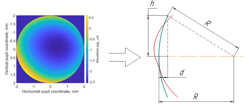
the average spherical curvature of the wavefront. Figure 3.3 illustrates an
example of the ocular wavefront and fitting of the mean spherical surface.
From the wavefront cross-section (Figure 3.3, right) we can write using the
Taylor series:
1 ℎ2
− = √ 2 + ℎ2 ≈ − ( ) ⋅ , (3.4a)
2 2
1 ℎ2
⇒ ≈ ( ) ⋅ . (3.4b)
2 2DESCRIBING AN OCULAR OPTICAL SYSTEM | 17 The , radius of the wavefront, can be then expressed as: ℎ2 = . (3.5) 2 If we know Zernike coefficients for the given wavefront, we can express d, the sag of the sphere, in terms of Zernike polynomials. Since we are describing a spherical surface, we are only interested in the term ( 2 + 2 ) of the wavefront representation. This term is present in the polynomials 0 , = 2, 4, 6.... Thus, for this spherical wavefront ℎ we can write: ℎ = ℎ ( ℎ , ℎ ), where the index ℎ indicates the radial height for which the sag is calculated (Figure 3.3). For the edge of the pupil we can write for the normalized coordinates x and y: = ℎ ( , )√ 2 + 2 =1 = √ √ = 20 ⋅ (2 3 ⋅ ( 2 + 2 )) − 40 ⋅ (6 5 ⋅ ( 2 + 2 )) + √ (3.6) + 60 ⋅ (12 7 ⋅ ( 2 + 2 )) − ... √ √ √ = 2 3 ⋅ 20 − 6 5 ⋅ 40 + 12 7 ⋅ 60 − ... , where 0 are Zernike coefficients in microns. As described earlier in this chapter, the refractive error refers to the required correction measured in diopters. To compensate for the curvature of the wavefront, we need a lens with effective back focal length ′ = − . Using the Equation 3.5 we can Figure 3.3. Illustrating calculations of refractive error using Zernike polynomials. Sketch on the right shows a vertical cross-section of the wavefront, depicted on the left. The red line represents the real wavefront surface, and green line shows the fitted spherical surface.
18 | DESCRIBING AN OCULAR OPTICAL SYSTEM
find the optical power of such lens, which is called the Spherical Equivalent
(SE):
1 1 −2 −2
[ ] = ′ = = 2 = 2 .
− ℎ
Finally, substituting from equation 3.6 we get:
√ √ √
4 3 12 5 0 24 7 0
[ ] = − 2 0
⋅ + 2 ⋅ 4 − 2 ⋅ + ... . (3.7)
2 6
The SE and spherical refractive error are linked by the relation:
= ℎ + . (3.8)
2
Described reasoning can be adopted to get the cylindrical lens power as
well. We can calculate projections of the cylindrical power on axes 0° and
45° and use these to find the cylinder and axis of the refractive error:
√ √
2 6 6 10 2 12√(14) 2
0 [ ] = − 2 2
⋅ + 2 ⋅ 4 − ⋅ 6 + ... , (3.9a)
2 2
√ √
2 6 6 10 −2 12√(14) −2
45 [ ] = − 2 −2
⋅ + 2 ⋅ − ⋅ 6 + ... , (3.9b)
2 4 2
2 ,
= −2√ 02 + 45 (3.9c)
⎧ = arctan ( + 2 0 ) ,
{
−2 45 (3.9d)
⎨
{if < 0, = + 180°.
⎩
3.4.3 Recalculating Zernike Coefficients for Different Wavelengths
In the human eye, the Zernike coefficients are commonly measured for the
near-infrared wavelengths (see Chapter 4). However, according to the ANSI
standard notation they should be given for = 0.55 m [28]. In order to re-
calculate Zernike coefficients for a different wavelength, the total wavefront
can be split into the spherical part and the residual wavefront perturba-
tions, represented as an additional phase plate. Then the total wavefront
for the measurement wavelength 1 :
Φ ( , ) 1 = Φ ℎ ( , ) 1 − ( 1 − 1) ⋅ Δ( , ), (3.10)
where Φ is the total wavefront deviations, Φ ℎ is the phase shift corre-
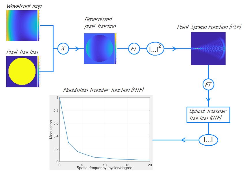
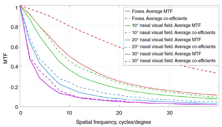
sponding to the SE, is the refractive index, and Δ is the phase plate of theDESCRIBING AN OCULAR OPTICAL SYSTEM | 19 residual wavefront. In this equation, the change of the wavelength can be accounted for by the change of refractive index . Thus, for the wavelength 2 : Φ ( , ) 2 = Φ ℎ ( , ) 1 − ( 2 − 1) ⋅ Δ( , ). (3.11) Substitution of Δ( , ) from Equation 3.10 into Equation 3.11 yields: Φ ( , ) 1 − Φ ℎ ( , ) 1 Φ ( , ) 2 = Φ ℎ ( , ) 1 + ( 2 − 1) = ( 1 − 1) ( 1 − 2 ) ( 2 − 1) = Φ ℎ ( , ) 1 + Φ ( , ) 1 . ( 1 − 1) ( 1 − 1) (3.12) The dispersion model described by Thibos et al. [29], for example, can be used to obtain the refractive index for different wavelengths. 3.4.4 Point Spread Function (PSF) and Modulation Transfer Function (MTF) Even though the Zernike coefficients describe the optics, they do not provide a direct quantitive assessment of the retinal image quality. For this purpose, the Papers A-F utilized the Modulation Transfer Function (MTF). The MTF, in its turn, is connected to the formation of the retinal image and the point spread function. A point spread function (PSF) can be thought of as an impulse response of the imaging optical system, that includes the influence of aberrations and diffraction. It shows the image that would result from a point source object. A spatially broad object can be represented as a superposition of multiple point sources. The retinal image is then a superposition of the PSFs resulting from each of the object points. Mathematically this is expressed as a convolution: = ( , ) , (3.13) where and are the intensity distributions in the object and image planes respectively. Equation 3.13 can be seen as spatial filtering, where the PSF is the filter that is smoothing out (blurring) the object details. The larger are the effects of aberrations and diffraction, the larger would be the blurring, which is equivalent to a spatially wide PSF. Thus, a narrow PSF corresponds to good image quality. Figure 3.4 shows an example of the PSF for a real eye and a diffraction limited PSF for the same pupil diameter. The PSF can be calculated from the so-called generalized pupil function, obtained for the entrance pupil of the optical system [27]. This function consists of two parts. One accounts for the wave aberrations, and one
20 | DESCRIBING AN OCULAR OPTICAL SYSTEM

 Figure 3.4. An example of the human eye PSF for 4 mm pupil diameter (left)
 and a corresponding diffraction limited PSF (right).

defines the shape of the pupil:
 ( , ) = ( , ) ⋅ exp (− ( , )) , (3.14)
where the ( , ) is the wave aberration, expressed as local optical path
differences, and ( , ) is the pupil function, which is equal to 1 within the
pupil and equal to 0 outside of it. The ocular wavefront maps, described in
the previous subsection, are thus the generalized pupil functions by defini-
tion. The PSF for the given image coordinate ( , ) is calculated from the
generalized pupil function as follows:
 2 ∗
 = ∣ { ( , )}∣ = { ( , )} ⋅ [ { ( , )}] , (3.15)
where is the generalized pupil function, {} is the Fourier transform,
and the asterisk denotes a complex conjugated function.
 The Modulation Transfer Function (MTF) is also broadly used as a
metric for the image quality. It utilizes the fact that the image blurring
created by diffraction and aberrations corresponds to contrast reduction for
features of different sizes. In simple, the MTF is a scaling factor for contrast
between the object and the image. The higher the MTF value, the better
the contrast transmission.

 Figure 3.5. Illustration of the spatial frequency in the MTF definition. Here
 1 > 2 and 1 < 2 .
DESCRIBING AN OCULAR OPTICAL SYSTEM | 21
Figure 3.6. An example of the surface-MTF (top row) and meridian-averaged
MTF (bottom row) for a 4 mm pupil diameter. The left column represents real
human eye while the right column depicts its diffraction limited analog. The
graphs correspond to the PSFs, shown in Figure 3.4.
By definition, MTF is a function of spatial frequency, which refers to
the periodic black and white lines (see Figure 3.5). The frequency is the
reciprocal of one full period of such a structure. The MTF value at the given
frequency is then the contrast scaling factor calculated for this periodic
structure as if located in the object plane. The spatial frequencies can be
expressed in linear units, lines per mm, or angular units, cycles per degree.
For the human eye, the MTF is normally given in cycles per degree to
avoid accounting for focal length of the eye, which has some population
variations. Figure 3.6 shows the MTF curves corresponding to the PSFs,
showed in Figure 3.4.
The MTF can be derived using the PSF. To do this we first have to define
the Optical Transfer Function (OTF) – the normalized Fourier transform
of the PSF. The OTF is calculated as:
{ } { }
( , ) = = ∞ , (3.16)
{ } ∣ ∬
=0, =0
−∞
where {} is the Fourier transform, and and are the horizontal and the
vertical coordinates in the image plane. The concept of the OTF is used to
bypass the calculation of the convolution in Equation 3.13 by taking Fourier22 | DESCRIBING AN OCULAR OPTICAL SYSTEM Figure 3.7. Diagram for calculating the PSF and the MTF from the ocular wavefront. Mathematical operations: X – multiplication, FT – Fourier transform, |…| – absolute value. transform of both parts of this equations. The OTF is not always positive. The negative values of this curve resemble the “contrast reversals” occurring for some spatial frequencies: the black-white structure of an object becomes a white-black structure in the image. The MTF is the absolute value of the OTF. Therefore, in contrast to OTF, the MTF is always positive. The normalization in Equation 3.16 renders (0, 0) = 1, which implies that the contrast scaling, given by the MTF, is relative to that for the zero spatial frequency. It should also be emphasized that in general, the MTF (as well as the OTF) is a function of frequencies in both the horizontal and the vertical direction ( and ). The conventional representation of MTF as a function of one frequency (with no direction) is obtained by averaging the MTF along all the meridians of the pupil. This meridian- averaged MTF therefore represents an average image quality for the object containing features oriented in all directions. To sum up this subsection, Figure 3.7 graphically represents the process of calculating the PSF and the MTF using the wavefront map of the human eye.
DESCRIBING AN OCULAR OPTICAL SYSTEM | 23

3.4.5 Contrast Sensitivity Function (CSF)
When it comes to analyzing vision, optics together with processing by the
retina and the brain should be taken into account. A rather comprehen-
sive representation of their combination is the Contrast Sensitivity Function
(CSF), that was studied in Paper A. As the name suggests, this function
describes how sensitive the eye is to the contrast of objects of different sizes.
The sensitivity is calculated as a reciprocal of the minimal contrast, required
to see features of a particular angular frequency. An example of a typical
CSF for the human eye is depicted on Figure 3.8. The angular frequency for
which CSF is zero corresponds to the resolution limit. Same as for the MTF,
the CSF is a function of horizontal and vertical frequencies, but it is also
usually analyzed as an average over the measured meridians. The two parts
of the CSF, that represent the optics and the image processing respectively,
are MTF and the Neural Contrast Sensitivity Function (NCSF):
 = ⋅ .
The NCSF accounts for the retinal image registration abilities. Earlier it
was rather laborious to measure MTF directly. But it could be calculated
using the CSF, obtained from psychophysical experiments, and the NCSF,
measured by projecting interference patterns on the retina to bypass the
ocular optics. With recent technological advancements, the situation has
changed: it is now the CSF and the NSCF that are more cumbersome to
measure. Therefore, for some tasks, a population average approximation of
the NCSF is often used. The appropriate tasks for such substitution include
retinal image quality metrics, described in the following section.

 Figure 3.8. A typical CSF for the human eye. Data from [30].
24 | DESCRIBING AN OCULAR OPTICAL SYSTEM

 Figure 3.9. The horizontal cross-section of the real (left) and diffraction-limited
 (right) PSF illustrating calculations of the encircled energy, the full-width at half-
 maximum, and the Strehl ratio.

3.4.6 Other Retinal Image Metrics
Although the PSF, the MTF and the CSF give a very comprehensive rep-
resentation of ocular optics and visual function, there are cases when their
usage is not optimal. In some applications it can be beneficial to highlight
or summarize some features instead of displaying all the data. Therefore,
there is a variety of adopted metrics for the retinal image quality, based on
each of these three fundamental concepts [31].

PSF-based Metrics
One way to assess the quality of the PSF is to look at the parameters
of this function. Figure 3.9 shows a vertical cross-section of two PSFs,
presented earlier on Figure 3.4. We can now choose a circle radius, smaller
than the PSF, and calculate the fraction of energy enclosed in this circle.
As mentioned before, a narrower PSF corresponds to better image quality.
Therefore, the fraction of encircled energy would be higher for the better
PSF. A similar concept is the Full Width at Half Maximum. It is assessing
the diameter of the circle at the fixed energy level – 50% of the maximum.
 The Strehl ratio illustrates how close the analyzed optical system is to
its diffraction limited analog. It is estimating the relative energy level at
peak of the PSF as:
 ( )
 = , (3.17)
 ( )
where both PSFs are normalized by the total PSF energy, and index “ ”
denotes a diffraction-limited optical system.
DESCRIBING AN OCULAR OPTICAL SYSTEM | 25

MTF- and CSF-based Metrics
Calculating the area under MTF or OTF allows to compress the description
of these functions down to just one number. It can be useful for working with
large amounts of data, when the comparison of the full curves is cumbersome
to perform or visualize. As the name suggests, the calculation of these two
metrics is performed as:
 ∞

 = ∬ ( , ) , (3.18a)
 −∞
 ∞

 = ∬ ( , ) , (3.18b)
 −∞

 The Visual Strehl Ration is the area under the weighted OTF, normal-
ized by its diffraction-limited analog. The weighing factor is the NCSF,
which implies that the OTF at some spatial frequencies is more important
for vision (has higher weighing factor) than OTF at other spatial frequen-
cies. Similar to the AreaMTF, the Visual Strehl Ratio compresses the OTF
assessment to only one number.
 ∞
 ∬ ( , ) ⋅ ( , )
 = −∞
 ∞ , (3.19)
 ∬ ( , ) ⋅ ( , )
 −∞

where the index “ ” denotes diffraction limited optical system. This defi-
nition is advantageous as the OTF function would give an additional penalty
for contrast reversals (negative OTF). However, OTF is a complex-valued
function, which is sometimes bulky to deal with. Therefore, some authors
suggest using an MTF instead of the OTF (and denote it respec-
tively) [32].
INSTRUMENTATION FOR THE WAVEFRONT MEASUREMENTS | 27

Chapter 4

Instrumentation for the
Wavefront Measurements

Measurements of the full aberrations of the human eye, once technologi-
cally challenging, are now commercially available. The most prevalent de-
vice for this kind of measurements is the Hartmann-Shack wavefront sensor
(HSWS). This chapter presents the principle of this sensor followed by the
description of two devices: the adaptive optics vision simulator, and the
dual-angle open field wavefront sensor. These devices were developed at
the Visual Optics group at the KTH University and they both incorpo-
rate a Hartmann-Shack sensor. The configuration of these devices allows to
perform a variety of different experiments, which cannot be done with the
currently available commercial systems.

4.1 Hartmann-Shack Wavefront Sensor

The principle of the HSWS measurements is illustrated in Figure 4.1. The
device consists of an array of identical microlenses, or lenslets, and a detector

 Figure 4.1. The principle of measurements in the HSWS. D - detector, MLA -
 microlens array, WF - incident wavefront.
28 | INSTRUMENTATION FOR THE WAVEFRONT MEASUREMENTS

at the back focal plane of this array. When a wavefront enters the sensor,
it first encounters the microlens array. Each of the microlenses cuts out a
small portion of the wavefront and images it onto the detector. Since the
detector is at the back focal plane of the lenses, the image of each small
wavefront part would be a spot. The location of the center of mass for such
a spot would indicate the average slope of the wavefront portion, imaged by
one lenslet. If the incoming wavefront is flat with no tilts, all of the spots
would be centered at the optical axes of their microlenses. If the incoming
wavefront is distorted, the spots would be shifted. This shift is proportional
to the focal length of the lenslets and to the local distortion of the wavefront.
The local slopes of the wavefront can be then back-calculated for horizontal
and vertical direction separately, and represent the local partial derivatives
of the wavefront. These partial derivatives are used to perform the least
square fit to the derivatives of the Zernike polynomials (Equations 3.2 in
Chapter 3).
 In order to use a HSWS for eyes, a measurement light is required. This
light is a monochromatic collimated narrow beam, usually in the near-
infrared spectrum, parallel to the optical axis of the HSWS. This beam
should enter the eye, reach the retina and create a point source at that
retinal location. The light from this point source, diffusely reflected back,
passes through the ocular optics and is finally registered at the exit pupil of
the eye. If the eye is aberrations-free, the captured wavefront will be flat.
 As it is physically impossible to locate the microlens array at the exit
pupil of the eye, an additional telescope is used. The exit pupil of the eye
acts as the entrance pupil of the telescope, and the microlens array is placed
at the corresponding exit pupil of the telescope. In this setting the angular
and linear magnifications between the two planes are constant irrespective
of the ocular wavefront.
 A HSWS can be used at different eccentricities of the VF: the sensor
together with the measurement light should be rotated around the center
of the eye’s entrance pupil.

4.2 Adaptive Optics Vision Simulator

The adaptive optics vision simulator at KTH University, developed by Rosén
et al. in 2012 [33], was used to perform measurements for Papers A, C and
E. It allows to induce and correct different amounts of aberrations and
test vision performance in these conditions. The schematic drawing of the
simulator is shown in Figure 4.2. The drawn setting illustrates off-axis mea-
surements in the nasal VF of the right eye. The subject is fixating foveally
on the target T using the left eye and views the screen (S) with visual
tasks with the right eye. Before reaching the eye, the light from the screen
INSTRUMENTATION FOR THE WAVEFRONT MEASUREMENTS | 29

 Figure 4.2. Schematic drawing of the adaptive optics vision simulator, developed
 by Rosén et al. in 2012 [33]. The setting illustrates off-axis measurements in nasal
 visual field of the right eye. BS – beam splitter; CCD – pupil camera; DM –
 deformable mirror; HM - hot mirror; HSWS – Hartmann-Shack wavefront sensor;
 L – lens; (L1 + L2), (L3 + L4) and (L3 + L5) – telescopes; LD – laser diode
 (measurement light), = 830 nm; M - mirror; S - screen with the vision evaluation
 stimuli; T – foveal fixation target.

passes a deformable mirror (DM), that is capable of inducing or correcting
ocular aberrations in a well-controlled manner in real time. The combined
aberrations of the eye together with the DM are constantly monitored by
the HSWS that can work in a closed loop with the DM. The CCD camera
is used for lateral and longitudinal alignment of the subjects prior to the
experiments. The telescope (L3 + L5) is slightly defocused which allows to
place the target S at optical infinity and at the same time partially compen-
sate the discrepancy between the measurement light wavelength, 830 nm,
and that used for the standard aberrations representation, 550 nm [28] (see
Chapter 3 for more details).
 It is advantageous to use the DM for vision correction. As an adaptive
optics component, DM is a continuous or segmented reflective surface, which
can be reshaped by small actuators behind it (see Figure 4.3, left). The
main advantage of the DM is that it does not have chromatic aberrations.
In other words, the optical path difference, induced by the mirror profile,
You can also read